Fast Radio Bursts as Probes of Magnetic Fields in Galaxies at
Abstract
We present a sample of nine Fast Radio Bursts (FRBs) from which we derive magnetic field strengths of the host galaxies represented by normal, star-forming galaxies with stellar masses . We find no correlation between the FRB rotation measure (RM) and redshift which indicates that the RM values are due mostly to the FRB host contribution. This assertion is further supported by a significant positive correlation (Spearman test probability ) found between RM and the estimated host dispersion measure (; with Spearman rank correlation coefficient ). For these nine galaxies, we estimate their magnetic field strengths projected along the sightline finding a low median value of . This implies the magnetic fields of our sample of hosts are weaker than those characteristic of the Solar neighborhood (), but relatively consistent with a lower limit on the observed range of for star-forming, disk galaxies, especially as we consider reversals in the B-field, and that we are only probing . We compare to RMs from simulated galaxies of the Auriga project – magneto-hydrodynamic cosmological zoom simulations - and find that the simulations predict the observed values to within the CI. Upcoming FRB surveys will provide hundreds of new FRBs with high-precision localizations, rotation measures, and imaging follow-up to support further investigation on the magnetic fields of a diverse population of galaxies.
Keywords:
radio transient sources – magnetic fieldsI Introduction
Fast Radio Bursts (FRBs) are milli-second duration pulses of radio emission, arising predominantly from extragalactic sources (Cordes & Chatterjee 2019, e.g.). The first burst discovered, subsequently named the Lorimer burst (Lorimer et al. 2007), revealed a new radio transient class with unprecendented power to probe cosmological questions of matter distribution, universal expansion, and (inter-)galactic magnetism due to their dispersion and rotation measures (Gaensler 2009; Macquart et al. 2010; Akahori & Ryu 2011; Macquart et al. 2015; Akahori et al. 2016, DMs, RMs; e.g.). Since the discovery of FRBs, their dispersion measure has already been used to search for answers to long standing questions. Works such as Macquart et al. 2020 and Simha et al. 2020 offer a nearly complete baryon census—finding baryons where they were once nearly impossible to detect. Galactic halos and the intergalactic medium (IGM) are now being backlit by the flashlights that are FRBs, illuminating the once “missing” matter.
FRBs also have potential to probe another influential property of the universe – magnetic fields (Piro & Gaensler 2018; Hackstein et al. 2019, e.g.). Many questions such as the origins of magnetic fields, their effects on the evolution of galaxies, and the process of their amplification over cosmological time have been explored extensively with theoretical treatments (Springel 2010; Pakmor et al. 2011; Rodrigues et al. 2018, e.g.). Observational constraints, however, are currently scant and are critically needed to constrain the physical processes at work.
There are a number of ways to measure the effects of magnetism in galactic and extragalactic systems, and each method is sensitive to a different magnetic field component (see Beck 2015 for a list of magnetic field components and observational methods). The Zeeman effect can be observed in the emission line spectra of galaxies, indicating a regular field along the line of sight. One can also measure the polarized intensity and linear polarization angle of QSOs and other persistent radio sources, or evaluate signatures from synchrotron radiation which are associated with the magnetic field component that is perpendicular to the line of sight.
In this study we use the Faraday rotation measures (RMs) —which quantify the effect of magnetized plasma on linearly polarized radiation— of FRBs to probe the component of the magnetic field which is parallel to the line of sight (). This measure can elucidate the magneto-ionic environment surrounding the FRB. As the signal also interacts with the inter-stellar and circum-galactic media of the FRB host, we can make measurements of the fields in these broader regions as well.
Constraining these field components helps determine what processes are implicated in the production and amplification of magnetic fields—whether tied to the progenitor object itself and its immediate environment (Piro & Gaensler 2018, e.g.) or evolution on galactic and cosmic scales (Hackstein et al. 2019, e.g.). Comparison of the observed quantities to those predicted by simulations, can be an invaluable test of our understanding of the relationship between magnetic fields and galaxy evolution (Rodrigues et al. 2018, e.g.). We can also test FRB progenitor models and how burst properties would be affected.
In this paper we make use of the Auriga simulations (Grand et al. 2017), a set of high resolution cosmological zoom-in simulations of Milky Way-like galaxies that reproduce many important properties of their observed counterparts. In particular they include a self-consistent model of magnetic field amplification and evolution over cosmic time that produces realistic magnetic field strengths at (Pakmor et al. 2017; Pakmor et al. 2018; Pakmor et al. 2020). We use the simulations to connect the FRB observations to conditions in their local and global environments of their host galaxies.
We also explore the possible connections between the RMs of a set of FRBs and local characteristics determined by, e.g., Heintz et al. 2020, Bhandari et al. 2020a, and Mannings et al. 2021. These works demonstrate that FRBs originate primarily in star-forming galaxies with stellar masses ranging from . These data also reveal the location of the FRBs within their hosts and constrain local measures such as the star formation density which may correlate with magnetized plasma.
This paper is organized as follows. We describe rotation measure in detail in Section I.1. In Section II, we outline the selection criteria for our sample (§II.1), provide a description of rotation measure data (§II.2), detail the host observations for each burst (§II.3), and describe host properties (§II.4). In Section III, we discuss the observational analysis and results. We begin by detailing the methods for estimating host contributions to RM and DM ( and ), including the extragalactic contribution to the rotation measure(§III.1), the Milky Way contribution to RM (§III.1.1), the correlation between rotation measure and redshift ( III.1.2), and estimates of (§III.2). We then investigate correlations between and host galaxy characteristics in Section III.3, and, in Section III.4, we make estimates of magnetic field magnitudes of the galaxies hosting the FRBs. We then discuss the modeling framework for and results for a magneto-hydrodynamic model of Milky Way-like galaxies (§IV, §IV.2) with which we simulate rotation and dispersion measure measurements and compare against observed values (§IV.3, and §IV.4). We finish with a final summary and discussion of implications in Section V.
I.1 Polarization and Faraday Effect
If the oscillations of an electromagnetic field have a preferred orientation, then this radiation is polarized. The polarization of an electromagnetic (EM) wave is determined by the orientation of the electric field component. In general, the polarization of an EM wave is elliptical, i.e. the electric field vector traces an ellipse perpendicular to the propagation direction during transit. Elliptically polarized light can be expressed as a linear combination of two orthogonal linear polarization states or two circular polarization states (Griffiths 2013). One requires only three independent parameters to describe the polarization state of an EM wave.
Polarization of radio waves, however, are most often described using the Stokes I, Q, U, and V parameters, where I refers to the total intensity, Q and U linear polarization, and V circular polarization. These parameters can be combined to represent polarization in the form of the Stokes vector
| (1) |
Estimating Q, U, and V from raw data depends on the specific configuration of the instrument used to detect and measure the polarization signals. As we are including FRBs from multiple experiments across multiple telescopes, descriptions of their methods and parameter formulations can be found in their respective studies (Michilli et al. 2018; Day et al. 2020; Mckinven et al. 2021; Kumar et al. 2022).
The linear polarization angle is expressed as
| (2) |
is, in general, a function of frequency and time, , and for FRBs it has been observed to evolve over the duration of the burst (Day et al. 2020; Michilli et al. 2018, e.g.).
As monochromatic light propagates through plasma which has a magnetic field component along the direction of propagation, its linear polarization angle is rotated. The degree of rotation is proportional to the inverse square of the frequency and the proportionality constant depends on the properties of the intervening magnetized medium. While the net rotation at any wavelength or frequency cannot be determined, for a multi-frequency radio signal like an FRB, the rotation measure () encodes the properties of the intervening medium and is measured from the variation of the linear polarization angle with wavelength squared:
| (3) |
For a pulse of radiation emitted at redshift z that traverses to Earth, we may express
| (4) |
where is a set of physical constants including the inverse square of the electron mass , electron charge cubed , and the inverse of the speed of light to the fourth power . is the electron density, is the magnitude of the line of sight magnetic field, and the integral is over the length of the sightline dl with and dl as functions of z. can be positive or negative depending on the direction of the magnetic field component. In other words, is the average parallel magnetic field strength along the line of sight weighted by . For FRBs, this includes contributions from the Milky Way, cosmic magnetic fields and the magnetic fields within its host galaxy.
However, it is assumed the field undergoes numerous reversals along the line of sight that minimize the IGM contribution to the RM relative to the host and Milky Way contributions. Our assumptions about the structure of the magnetic field means that our interpretations of RM and derived quantities become model dependent. Nonetheless, there exist measurements of RM in cosmic filaments () such as those presented in Carretti et al. 2022, which provides estimates around . They then infer a magnetic field magnitude in the filaments to be . This value being a tenth of an RM unit (and assuming the value in cosmic voids is even lower due to a lack of ionized material in these regions) motivates an expectation for minimal RM contribution from the IGM. Specific to FRBs, upper limits on the CGM and IGM contributions to FRB Rotation measures, can be found in Ravi et al. 2016; Prochaska et al. 2019 and O’Sullivan et al. 2020.
Maps of the Milky Way’s magnetic field and Faraday rotation have been developed using measurements of extragalactic polarized sources, as discussed in Section III.1.1. Once this contribution is subtracted, we can isolate the other components in an effort to better understand magnetic field generation and amplification in the universe, as well as the magneto-ionic environments of FRB progenitors.
| FRB | / | Refs | |||||
|---|---|---|---|---|---|---|---|
| () | () | () | () | ||||
| 20121102A† | 558 | 0.193 | (1),(2) | ||||
| 20180916B† | 349 | 0.034 | — | (2),(3),(4) | |||
| 20180924B | 362 | 0.321 | (2),(5) | ||||
| 20190102C | 365 | 0.291 | (2),(6) | ||||
| 20190608B | 340 | 0.118 | (2),(6) | ||||
| 20190711A† | 588 | 0.522 | (2),(6) | ||||
| 20191001A | 508 | 0.234 | (2),(7) | ||||
| 20200120E† | 88 | 0.001 | — | — | (8) | ||
| 20201124A† | 411 | 0.098 | — | — | (9) | ||
Note. — FRB is the TNS name of the fast radio burst. Those with a dagger are known to repeat. is the rotation measure of the FRB. is the dispersion measure of the FRB rounded to the nearest whole number. Uncertainties are generally less than 1. is the redshift of the FRB. / is the physical offset of the FRB from the host galaxy center in units of effective radii (host-normalized offset). is the stellar mass surface density of the host galaxy at the FRB location. is the specific star formation rate of the host galaxy at the FRB location. FRBs without or values do not have imaging necessary to compute these quantities, and were not reported in Mannings et al. 2021. Refs are the references: (1) Michilli et al. 2018 (2) Mannings et al. 2021 (3) Tendulkar et al. 2020 (4) CHIME/FRB Collaboration et al. 2019 (5) Bannister et al. 2019 (6) Day et al. 2020 (7) Bhandari et al. 2020b (8) Bhardwaj et al. 2021 (9) Kumar et al. 2022
II FRB Data and Sample Selection
II.1 Selection Criteria
Presently, there are over 600 FRBs in the published literature and of these with published values. These form the parent sample from which we construct a subset for our analysis. Our scientific foci are to:
- •
Study correlations between local host properties and the inferred host contribution to the RM.
- •
Estimate magnetic fields in FRB hosts.
- •
Make comparisons to cosmological zoom-in simulations that study the relationship between galaxy evolution and magnetic fields.
These scientific goals helped define the following selection criteria that each FRB must satisfy:
- 1.
A precisely measured value.
- 2.
A kpc-scale FRB localization precision.
- 3.
A high probability association to a host galaxy.
- 4.
A spectroscopic redshift measurement for the host galaxy.
- 5.
Host galaxy imaging and subsequent derived host properties. such as stellar mass, star-formation rate, etc.
- 6.
Considered and added to the sample by January 2022.
The first criterion is fundamental to the analysis. The second addresses the fact that RMs are sensitive to turbulent small-scale magnetic fields as well as large-scale ordered fields. Requiring kpc-scale localizations allows an exploration of correlations between local measures such as the star-formation rate surface density and . In the following analysis, we require the net localization uncertainty (statistical and systematic error) be less than 5 kpc at the redshift of the host galaxy.
Regarding the third criterion, we adopt the Probabilistic Association of Transients to Hosts (Aggarwal et al. 2021, PATH;) formalism and demand that the FRB posterior probability exceeds 95%. In general, this criterion is redundant with the second as a highly precise localization will generally yield a secure association provided sufficiently deep imaging (Eftekhari et al. 2020). The fifth and sixth criteria allow us to search for correlations between the host galaxy properties and .
After applying these selection criteria to the full set of published sources, we recover 9 FRBs satisfying the full set. These are listed in Table 1.
II.2 Rotation Measures and Other Burst Properties
The 9 FRBs defining our sample are drawn primarily from two FRB surveys. The first is the Commensal Real-time ASKAP Fast Transients (CRAFT) survey using the Australian Square Kilometre Array Pathfinder (ASKAP) telescope Macquart et al. 2010. The CRAFT collaboration discovered and observed six of the FRB events presented in this paper, on the date in accordance with the TNS name of the event: 20180924B (Bannister et al. 2019), 20190102C, 20190608B, 20190711A (Day et al. 2020), 20191001A (Bhandari et al. 2020b), and 20201124A (Kumar et al. 2022). 20190711A and 20201124A are repeating bursts whose rotation measure may change with time; the quoted rotation measures are taken from the publications in which these data are presented which are the first detected burst and an average over all detected bursts, respectively.
Two of the bursts in this sample were detected and characterized by the Canadian Hydrogen Intensity Mapping Experiment (CHIME)/FRB Experiment (FRBs 20180916B, 20200120E). The rotation measure for FRB 20180916B—located in a nearby spiral galaxy (Tendulkar et al. 2020)—is presented by the CHIME collaboration with 7 other new (at the time) repeating FRBs (CHIME/FRB Collaboration et al. 2019). The RM for this burst was derived from baseband data collected on FRB 20181226A, a subsequent repetition of FRB 20180916B. FRB 20200120E is localized to a Globular Cluster located in the halo of M81 and is presented in Bhardwaj et al. 2021.
Lastly, we include the source commonly referred to as “The Repeater” or R1: FRB 20121102A. The rotation measure for FRB 20121102A was first presented in Michilli et al. 2018, which detailed the extreme magneto-ionic environment in which the burst progenitor must be embedded, in order to produce such a high rotation measure, . Since this is a repeating burst we take the average quoted in Michilli et al. 2018 as our value.
Five out of the 9 FRBs in this sample repeat, leaving four apparently non-repeating bursts. The sample has a median with a range (see Table 1).
Repeating bursts can show variability and evolution over the individual burst envelope and with time over subsequent burst repetitions (Michilli et al. 2018, e.g.). All of the repeating bursts in the sample show at least slight variability in their RMs from burst to burst. These variations are insignificant in comparison to the FRB source to FRB source variation in and do not impact any of the analysis presented here.
| FRB | RAFRB | DecFRB | RAHost | DecHost | SFR | ||
|---|---|---|---|---|---|---|---|
| () | () | (kpc) | |||||
| 20121102A† | 82.9946 | 82.9945 | 0.13 | ||||
| 20180916B† | 29.5031 | 29.5012 | 0.06 | ||||
| 20180924B | 326.1052 | 326.1052 | 0.88 | ||||
| 20190102C | 322.4157 | 322.4149 | 0.86 | ||||
| 20190608B | 334.0199 | 334.0204 | 0.69 | ||||
| 20190711A† | 329.4192 | 329.4192 | 0.42 | ||||
| 20191001A | 323.3513 | 323.3518 | 8.07 | ||||
| 20200120E† | 149.4778 | 148.8882 | 0.89 | ||||
| 20201124A† | 77.0146 | 77.0145 | 2.10 | ||||
Note. — FRB is the TNS name of the fast radio burst; those with a dagger are known to repeat. RAFRB,DecFRB are the coordinates of the FRB. RAHost,DecHost are the coordinates of the host galaxy. is the stellar mass of the host galaxy. SFR is the star formation rate of the host galaxy, with typical uncertainty of 30% (systematic). is the effective radius of the host galaxy.
II.3 Host Observations
Nearly all of the observations of the host galaxies for our RM sample have been published previously. Here we briefly review the primary datasets.
Regarding imaging, where available we have leveraged high-spatial resolution data obtained with the Hubble Space Telescope (HST). Six of the hosts in the sample were observed by HST and its Wide-field Camera 3 (WFC3) in UVIS and IR images (F300X and F160W filters, respectively) taken as part of GO programs 15878 (PI: Prochaska) and 16080 (PI: Mannings).
These programs targeted galaxies for which FRB events have been detected and localized by the CRAFT survey. These images were previously published in Chittidi et al. 2021 and Mannings et al. 2021. Information for FRBs 20180924B, 20190102C, 20190608B, 20190711A, and 20191001A was drawn from this dataset.
We also include HST images from GO program 14890 (PI: Tendulkar) which observed the host of FRB 20121102A (Bassa et al. 2017). These observations include images taken in the F110W and F160W IR filters (equivalent to J and H bands, respectively), and a narrow-band H- image with the F763M filter. Detailed descriptions of image processing and reduction can be found in Bassa et al. 2017 and Mannings et al. 2021.
The high spatial-resolution imaging is complemented by multi-band, ground-based images from public surveys and directed follow-up campaigns. We refer the reader to Heintz et al. 2020 and Bhandari et al. 2020a; Bhandari et al. 2020b; Bhandari et al. 2022 for details and note the data are all taken from the FRB repository on GitHub (Prochaska et al. 2019).

II.4 Host Properties
Central to our study is an exploration of the properties of the galaxies hosting the FRBs, both global and local measures. We use the quantities derived from previous studies throughout this work: star-formation rates (global and local to the FRB, SFR and ), effective radii (), stellar mass (global and local to the FRB), and offsets. These are tabulated in Tables 1 (local properties) and 2 (global galaxy properties).
Figure 1 shows the locations of the FRBs within their host galaxies relative to the host galaxy centroid and in units of . We have de-projected the offsets along the major and minor axes using fits to each host with the galfit (Peng et al. 2010) software package. Most of which are reported in Mannings et al. 2021, with the remaining two fits being presented here (FRBs 20200120E and 20201124A).
We observe that most of the bursts are located within from the centers of their hosts, with one burst residing further out in its host’s disk at . Furthermore, Mannings et al. 2021 characterizes the FRB locations in that sample as occurring at moderate offsets on or near spiral arm structure. Bhardwaj et al. 2021 shows that FRB 20201001E likely originated in a globular cluster in the outskirts of M81. In contrast, FRB 20121102A occurs very near a central star-forming region in its host. Therefore, as regards the ISM contribution to the , one expects variation as the bursts occur in relatively diverse environments although the majority are located on or near spiral structure.


We also characterize the host galaxies in the sample according to their overall properties. In Figure 2, we compare the global properties of the host galaxies in the sample against measurements of field galaxies at similar redshift. In the bottom panel, we show a color-magnitude diagram where hosts in the “Blue” region are early-type galaxies with young stellar populations and active star-formation, while those in the “Red” region are late-type hosts with very low star-formation and older stellar populations. The majority of these FRB hosts are star-forming and lie either in the so-called blue-cloud of galaxies or the green valley, as supported by what is shown in the upper panel (the star-formation rate vs stellar mass diagram) where most of the hosts reside in the ”star-forming” region of the plot. The two notable exceptions are FRB 20200120E and FRB 20180916B which have hosts with non-zero SFR but lie below the SFR main-sequence, The figure indicates that the galaxies studied here have properties typical of a population with a preference for star-forming and more luminous/massive galaxies. For the full parent population of FRB host galaxies, however, Safarzadeh et al. 2020 demonstrated that the hosts are less massive (and have lower SFR) than a sample weighted by SFR. The points are colored by the extra-galactic RM (; see eq.5), but there is no apparent correlation between the host properties and .
III Observational Analysis and Results
In this section we analyze the measurements to search for correlations with the host galaxy properties and to estimate the underlying magnetic fields within the hosts. We begin by introducing approaches to isolate the RM and DM contributions from the host.
The host and burst characteristics for FRB 20121102A are anomalous in comparison to the rest of the sample, as the host is a star-forming dwarf with a persistent radio source, and the burst’s is orders of magnitude higher than other bursts in this sample. Much attention has been given to FRB 20121102A with respect to its high , in an attempt to determine what connection this value has to possible progenitor channels and local magnetic field properties.
It should be noted that the of 20121102A is not completely unique with the detection of FRB 20190520B (Zhao & Wang 2021; Niu et al. 2022) whose and are both much higher than what has been observed with other bursts. The varies substantially, but reaches a maximum (Anna-Thomas et al. 2023), and the progenitor argued to be embedded in a combined magnetar wind nebula and supernova remnant (Zhao & Wang 2021). We include FRB 20121102A in our analysis despite its extreme RM, but, where relevant, we comment on results without its inclusion.
III.1 Constraining the Contribution to from the IGM
In this subsection, we search for any trend of with redshift akin to the Macquart Relation for the dispersion measure.
In this case we do not expect a trend with redshift since there is no expected preferred direction of magnetic fields on cosmic scales. The random orientation of these intergalactic fields, and probable dominance of the turbulent field components, leads to field reversals along what can be considered to be a random walk— where the mean field is , while . Therefore, integrated along the line of sight, approaches zero on average (§I.1). We first, however, describe our approach to removing an estimated contribution to from our Galaxy.
III.1.1 Milky Way Rotation Measure ()
Each of the measurements include a contribution from the path through our galaxy. This includes both the interstellar medium and any halo component.
The Faraday map presented in Oppermann, N. et al. 2012 uses surveys of polarized extragalactic radio sources to determine rotation measures within and outside of the Galactic plane.
This model’s methodology and theoretical framework is used as a basis for the production and improvement of the HE20 model (Hutschenreuter & Enßlin 2020; Hutschenreuter et al. 2022)—a Faraday sky model that uses the correlation between Galactic Faraday rotation and Galactic free-free emission to increase the accuracy of previously developed maps (Hutschenreuter & Enßlin 2020). They also incorporate a new all-sky data set, which has a higher density of sources near the galactic plane and other under-resolved areas of the sky (such as the southern sky). These improvements increase the resolution of the resulting maps by a factor of two over previous studies (Hutschenreuter et al. 2022).
Therefore, we use the HE20 model of to account for the Milky Way’s contribution to to thereby isolate the extragalactic RM contribution:
| (5) |
Last, we note that maps such as these are limited in their spatial resolution in regards to particular lines of sight through the Milky Way. However, the HE20 model uses a total of 55,190 sources (primarily from the LOFAR Two-metre Sky Survey and NRAO VLA Sky Survey RM catalogs), resulting in improvements in resolution and uncertainties. The uncertainties mostly range from in the plane of the galaxy to as we move to lines of sight further from the disk. There are few regions in the Galactic plane (specifically towards Galactic center) where the uncertainties reach (Hutschenreuter et al. 2022), but none of our FRBs have LOS near .

III.1.2 Correlating with
Figure 3 plots the absolute value of the extragalactic for each sightline against the FRB redshift. There is no discernible trend between these two quantities. Both parameter (slope of the best-fit line) and non-parametric (Spearman) tests reveal no significant correlation. This stands in stark contrast to the strong correlation observed between DM and redshift (the Macquart relation), which arises from the highly ionized cosmic web (Macquart et al. 2020). The absence of any apparent correlation in Figure 3 implies the IGM makes little contribution to the overall RM, primarily due to reversals in the magnetic field over cosmic scales. This is consistent with upper limits for the contribution of intervening galaxy halos (Lan & Prochaska 2020).
For the remainder of the paper, we assert that the cosmic contribution to () is negligible. Therefore is dominated by only two components along the sightline, our Galaxy and the FRB host. In turn, this implies is dominated by the host contribution and given equation 5 we have,
| (6) |
which explicitly applies a factor of to correct to the host rest-frame. In what follows, we test equation 6 and then derive estimates for the magnetic field strength of the FRB host galaxies based on its evaluation.
III.2 Estimating the Host Dispersion Measure ()
| FRB | ||||||
|---|---|---|---|---|---|---|
| () | () | () | () | () | () | |
| 20121102A† | 183 | 3519 | ||||
| 20180916B† | 167 | |||||
| 20180924B | 311 | |||||
| 20190102C | 177 | |||||
| 20190608B | 135 | 154 | ||||
| 20190711A† | ||||||
| 20191001A | 512 | |||||
| 20200120E† | ||||||
| 20201124A† | 810 | |||||
Note. — Daggers denote repeating FRBs. for FRBs 20180924B, 20190102C, and 20200120E are all below 30.For the calculation of we set a minumum DM of 30 , but report the derived values here. Those left blank do not have the necessary measurements to calculate using the particular method.
In section III.1.2, we argued that the extragalactic RM () estimates for the FRBs arise from ionized and magnetized gas within their host galaxies. Adopting this expectation, we may leverage observations of the galaxies and the local environments of the FRBs to provide further insight into the underlying magnetic field. In particular, we aim to provide an order-of-magnitude estimate for the magnetic field strength. Following standard treatment for sightlines through the Galactic ISM (Arshakian et al. 2009; Beck et al. 2019, e.g.), one requires an estimate for the dispersion measure of the gas giving rise to to calculate . We will also use this DM estimate to guide the models of presented in Section IV.
We will make the further assumption that is dominated by gas within the host galaxy ISM and/or the local environment of the FRB. Specifically, we ignore any RM contribution from the diffuse and ionized gas of the host halo. This is due to the lower anticipated density of halo gas, as supported by galaxy formation theory and simulations (see IV). Therefore, we wish to estimate the dispersion measure of the host foreground to the FRB. We define this quantity as and assume that .
We consider several approaches to estimate , each of which bears significant uncertainty. One approach follows Reynolds 1977 (further developed in Tendulkar et al. 2017) who introduced a method to relate the emission measure EM () to the sightline DM () allowing for a parameterization of the unknown clumping of the gas. For EM, we consider two observed fluxes of radiation from gas towards the FRB.
The first EM is the observed surface brightness of Hydrogen recombination radiation (e.g. ). In its favor, the majority of FRB host galaxies have one or more optical, nebular Hydrogen recombination lines measured from optical spectroscopy (Bhandari et al. 2022, e.g.). On the negative side, most of these were obtained from long-slit observations centered on the host galaxy and not necessarily including the FRB location. Furthermore, the typical atmospheric seeing of and the generally small angular sizes of the galaxies (with exceptions) yield only a characteristic surface brightness from the host galaxy ISM. Table 3 lists a set of estimates of based on published, integrated flux measurements11 1 Or converted to using standard nebular flux ratios., the angular sizes of the galaxies, and corrected for dust extinction. These range from one to many hundreds .
For the subset of FRBs with hosts observed at high spatial resolution, we may better constrain the emission measure at the FRB location. Six of the 9 FRBs have extant Hubble Space Telescope (HST) observations at FWHM resolution (Mannings et al. 2021). These are primarily broadband images at UV and near-IR wavelengths. The UV emission is dominated by radiation from massive stars which also drive the nebular Hydrogen emission and the two are strongly correlated (Calzetti 2001, e.g.). For those with UV, we use the standard scaling between near-UV luminosity and luminosity (Kennicutt 1998) to estimate the surface brightness from the UV observations. We then calculate the emission measure and relate this to a dispersion measure estimate. Table 3 lists the estimates for these six galaxies.

Last, we consider a complementary approach to estimating using the Macquart Relation which relates the cosmic dispersion measure with redshift (Macquart et al. 2020). We refer to this estimation as . The method is to subtract from the observed total dispersion measure estimates for the Galactic ISM and halo (, ) and the cosmic web ():
| (7) |
We use the NE2001 model (Cordes & Lazio 2003) of the Galactic ISM to evaluate for each FRB sightline and assume the Milky Way halo contributes (Prochaska & Zheng 2019, e.g.). From the host galaxy redshift, we calculate the average (Macquart et al. 2020). This yields the values listed in Table 3 which have also been corrected to the rest frame of the host (i.e. we applied a factor of 1+). Formally, these include gas from both the ISM and halo of the host galaxy and current work suggests the host halo term may contribute several tens (Prochaska & Zheng 2019). We also note that structure in the cosmic web lends to an asymmetric scatter about and the median value is predicted to be several tens lower than the mean. These two corrections offset against one another, and we therefore proceed with equation 7 for our estimates acknowledging that these bear uncertainty.
Inspecting the values of listed in Table 3, one notes each approach exhibits a distinct distribution. The estimations span the largest range and exhibit the largest values. Indeed, many exceed and even the total of the sightline. The dust-corrected distribution are primarily upper limits of one hundred to a few hundreds and are generally consistent with . We proceed with analysis that adopts for the host dispersion measure, however of the values calculated for are or negative. Therefore we impose a minimum value of 30 based on the minimum value of our own Galactic ISM (NE2001), noting that all of the galaxies exhibit signatures of star-formation and must harbor a non-negligible ISM. This minimum value also accounts for uncertainty in the methodology. For completeness, the values presented in Table 3 show the calculated values for including those which are below this minimum. However, the minimum threshold is implemented in all subsequent analysis.
III.3 Correlating Host Characteristics with Rotation Measure
We now test for correlations between global and local characteristics of the host galaxies and RM isolated to the host galaxy (i.e. with the Galactic component subtracted using equation 6; ). To the extent that traces gas beyond the local environment, we may identify correlations with the host galaxy properties. For example, one may expect FRBs found in regions of elevated star-formation to exhibit a higher rotation measure. Magnetic fields get wrapped up into forming stars, but the fields can also be amplified by ionizing radiation and turbulence from violent star formation, cloud collapse, and massive star death.
Specifically, we consider global measures of the star-formation rate (SFR), stellar mass (), and galacto-centric offset (relative to the galaxy effective radius, ). We also consider local measures of the SFR and surface densities (, ; Table 1) and our estimate of which would include both local and ISM contributions.
We perform Spearman tests - computing Spearman correlation coefficients - with the null hypothesis that there is no correlation between rotation measure and a given measurement. We select the Spearman test because there is no assumption of Gaussian distributions for the variables. We perform the analysis in log-log space (as opposed to linear space) as the power-law relationships appear linear, and many of these values span several orders of magnitude. Last, we set a threshold of the Spearman probability for a significant correlation at (i.e. requiring 95% significance).
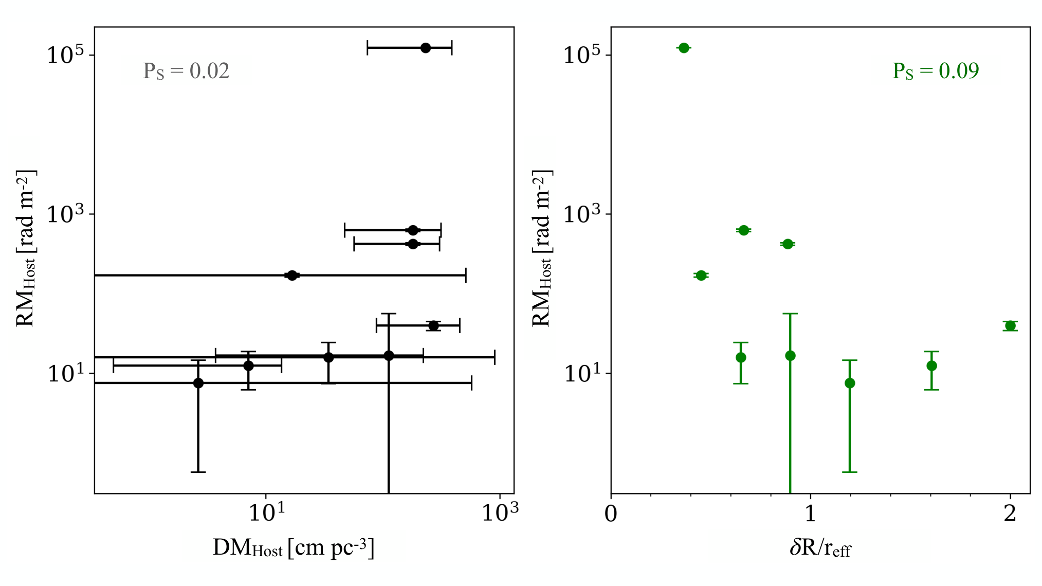

The absolute values of the resultant values are shown in Figure 4. Although there are a number of parameters for which , the condition for significance is only satisfied for one quantity: . A positive correlation between and is in line with expectation because both quantities depend on the electron density of the host ISM. The correlation also lends further support to the assertion that is dominated by .
The next strongest correlation is an anti-correlation between and , although with . This trend follows observed and simulated inverse relationships between and radius (Wielebinski & Beck 2005; Pakmor et al. 2017, e.g.). We await future observations to confirm (or refute) such a trend in FRB observations.
As our sample is limited a sample size of 9 FRBs, such tests should be repeated with greater confidence with a larger sample size. One also notes that the significance of these analyses is reduced by a trials-factor penalty incurred when testing for multiple correlations.
III.4 B-field Estimation
As stated in Arshakian et al. 2009, rotation measures of polarized background sources can be used to reconstruct a host or intervening galaxy’s magnetic field topology. FRB signals have since been shown to be one such source. FRBs and their rotation measures can reveal the orientation and magnitude of ordered magnetic fields, making them a powerful tool. Here we look at the power of FRB sightlines to provide insight on the fields of the galaxies that host well-localized bursts.
As defined, is the sightline integral of the parallel component of the magnetic field weighted by the electron density. Therefore the ratio of RM to DM (the unweighted integral) yields an estimate of the magnetic field, after accounting for differences in the prefactors (Akahori et al. 2016; Pandhi et al. 2022, e.g.):
| (8) |
with and constants equal to 1000 and 811.9, respectively. In Akahori et al. 2016 they propose (with some improvements to equation 8) that many measurements of and can provide the data necessary to probe inter-galactic magnetic fields (IGMFs). This estimation also assumes a constant magnetic field and that there is no correlation between and , whereas it is possible the magnetic field strength will likely decrease exponentially with radius and height in the disk (similar to ). These effects should be less than an order of magnitude making the given ratio sufficient for estimating the magnitude of the magnetic fields in our sample’s host galaxies. Furthermore, we adopt values of and to isolate the magnetic field estimation to within the host galaxy.
Considering the turbulence and ionization due to active star-formation and the deaths of massive stars, one may suspect a relationship between star-formation rate and the magnitude of magnetic fields in the host. We also investigate the relationship between stellar mass and magnetic field strength. In Rodrigues et al. 2018—for galaxies at —they find a slight positive correlation between galaxy mass and magnetic field, but note that this correlation is broken by a number of lower-mass hosts with much higher magnetic field strengths. In Figure 6, we do not see a clear trend with strength as a function of mass nor star-formation rate, in contrast to the predictions of Rodrigues et al. 2018. FRB 20121102A exhibits the highest rotation measure of all the bursts, but resides in the lowest-mass host. This is indicative of the highly magnetized environment that the burst progenitor lives within (Michilli et al. 2018).
In most cases, the magnetic field strengths estimated are lower than values quoted for the Milky Way ( in the outer reaches of the galaxy and in the inner region towards the bulge). These Galactic values are dominated by the small-scale random fields which contrasts the regular fields along the line of sight that dominates RM. Comparing these two sets of measurements allows us to make distinctions between the strengths of various field components. We note that the values we have determined are largely consistent with field magnitudes, which is broadly accepted as the general magnitude of large-scale regular fields measured in galactic disks (Beck et al. 2019).
IV Modelling Galactic Magnetic Fields
IV.1 Auriga Model
To gain a better understanding of the physical mechanisms that can influence the magnetic fields in the host galaxies of our observed FRBs, we compare them to similar galaxies in the Auriga simulations.
The Auriga simulations are a set of cosmological magneto-hydrodynamical zoom-in simulations of Milky Way-like galaxies (Grand et al. 2017). They model magnetic fields in the approximation of ideal magnetohydrodynamics (MHD) using a second order finite volume scheme (Pakmor et al. 2011; Pakmor & Springel 2013) in the Arepo code (Springel 2010; Pakmor et al. 2016; Weinberger et al. 2020). The magnetic field is initialised at as a uniform magnetic seed field with a strength of . The simulation then evolves the magnetic field self-consistently until .
When the galaxies first form, the magnetic field is quickly amplified via a turbulent small-scale dynamo and saturates before with a magnetic energy density that reaches of the turbulent energy density and erases any information about the seed field in the galaxy (Pakmor et al. 2014). After the galaxies form a disk at the differential rotation in the disk leads to a second phase of magnetic field amplification that ends when the magnetic energy density reaches equipartition with the turbulent energy density (Pakmor et al. 2017). The magnetic field properties, synthetic Faraday rotation maps, and the magnetic field in the circum-galactic medium of the Auriga galaxies has been shown to be consistent with observations (Pakmor et al. 2016; Pakmor et al. 2018; Pakmor et al. 2020).
| FRB | RM Median | DM Median | ||
|---|---|---|---|---|
| () | () | () | () | |
| 20121102A† | 2.02 | 2.02 | [0.04,18.56] | [0.04,18.56] |
| 20180916B† | ||||
| 20180924B | 146.22 | 57.31 | [6.01,12598.00] | [4.20,117.59] |
| 20190102C | 53.55 | 7.24 | [0.63,1055.81] | [0.28,69.17] |
| 20190608B | 25.84 | 25.84 | [1.80,120.41] | [1.80,120.41] |
| 20190711A† | 8.58 | 1.66 | [0.00,745.50] | [0.00,97.79] |
| 20191001A | 77.71 | 77.71 | [3.40,635.87] | [3.40,635.87] |
| 20200120E† | ||||
| 20201124A† | 86.13 | 67.51 | [2.83,837.41] | [2.04,789.91] |
Note. — Daggers denote repeating FRBs. The data included here are taken from the Auriga simulations. No matches were found for FRBs 20180916B and 20200120E, thus they have been left blank.
The Auriga simulations focus on a Lagrangian high-resolution region with a typical radius of around the central Milky Way-mass galaxies. This high-resolution region contains a large number of smaller galaxies without contamination from low-resolution dark matter particles that we also include in our sample here. We focus our analysis on the six high-resolution simulations of the Auriga project with a baryonic mass resolution of . These are supplemented by yet unpublished simulations with the same mass resolution, centred on lower mass galaxies ( M⊙) for which the high-resolution regions also extend to about 5 times the virial radius around each central galaxy.
IV.2 Host and sightline selection
We first find galaxies in our simulation suite with stellar mass, star formation rate, and effective radius consistent with the host galaxies of our FRB sample. We calculate the stellar mass of a simulated galaxy by including all stars within three times its stellar half mass radius. Its star formation rate is averaged over the last 100 Myr using newly formed stars within the same radius. We use the stellar half mass radius as a proxy for the effective radius. We include all galaxies (both central and satellite galaxies) that match the FRB sample to within twice the observational error. For the effective radius, however, we add a 10 per cent error in quadrature to the observational error, because in some cases the derived errors were so small that no match could be found. With this selection procedure, we found one or more matching galaxies for out of the observed host galaxies.
We tilt each of the galaxies into the observed inclination and then integrate the RM and DM values for different lines of sight. The starting point of each line of sight is the position of a random star particle with an age younger than . The frequent incidence of FRBs one or near spiral arms, could indicate the association of FRBs with relatively young stellar populations. From the starting point we integrate each line of sight until it reaches an observer at a distance of . We checked that increasing the integration distance does not change our results.
The local electron density for the integration along the line of sight is computed exactly as described in Pakmor et al. 2018, in particular assuming that only the volume-filling warm phase of the ISM contributes and that this phase is fully ionised. The magnetic field is taken directly from the simulation.
IV.3 Correlation between DM and RM
We show the correlation between RM and DM for all sightlines we computed from the Auriga galaxies in Figure 7. RM and DM are clearly strongly correlated, as expected. However, there is significant scatter, i.e. for a fixed DM value the RM value can vary by two orders of magnitude. Nevertheless, the scatter is small on the scale of the overall variation of five orders of magnitudes in DM and eight orders of magnitude in RM.
Motivated by the strong correlation between DM and RM we not only compare the RM distributions of all lines of sight of matched FRB host galaxies, but also compare to a subsample of lines of sight that show consistent DM values.
IV.4 DM and RM of matched Auriga galaxies
We show the distribution of RM (purple lines) and DM (red lines) values for lines of sights each of all galaxies in our sample consistent with the properties of the FRB host galaxies in Figure 8. We also show the measured values as vertical lines of the same color.
Strikingly, the shape of the distributions of synthetic DM and RM values match for most FRBs. The RM and DM distributions overlap with the values inferred for the FRB host galaxies from our observations with the exception of FRB20201124A. Median values and 95% confidence intervals are shown in Table 4.
We also show the RM distributions restricted to lines of sights that have a DM value consistent with the observed host galaxy DM (, shown by the dashed, yellow curves). For most FRBs this restricted RM distribution is essentially the same as the full RM distribution. For FRB20190102C, FRB20201124A, and FRB20190711A this restriction reduces the high RM tail of the distribution. Interestingly, in all three cases the host RM estimated from observations lies on this tail that is reduced significantly by the restriction on DM. We also note (as seen in Figure 8) the noticeable difference between the modeled PDF and observed for FRB20190608B. Though, again the value lands on the tail of the distribution. This could point to an non-negligible contribution of the local environment to the observed RM, as was discussed in Chittidi et al. 2021. The authors point out the high RM in comparison to other bursts such as FRB 20180916, implying a magnetised local environment.
A larger sample is necessary to determine whether or not these variations are truly due to local effects.
An extreme exception is FRB20121102A. We do not find any lines of sight that have an RM value even remotely comparable to the large observed value. In contrast, the DM value is barely consistent with our synthetic lines of sight. This indicates that the magnetic field dominating the RM of FRB20121102A is part of its local stellar environment that is not included in our simulations. Michilli et al. 2018 discusses this highly magnetized local environment.
Note also, that it is likely increased scatter broadening of the FRB signal would bias against FRBs being detected with high host DM contribution.
V Discussion
This sample represents the largest collection of FRB rotation measures presented with accompanying high-precision localizations and follow-up imaging of the associated hosts. A majority of the hosts in this sample are massive, star-forming galaxies at , with a few exceptions at lower mass or SFR.
To explore the relationships between FRB rotation measures and host characteristics, we first isolated the extragalactic contribution to the rotation measure (). We used the Galactic Faraday rotation map developed in Hutschenreuter et al. 2022 and found no correlation between and . This is consistent with measurements of the IGMF found in Carretti et al. 2022 which follows from an expected random nature and much lower strength of the fields in the IGM.
We therefore disregarded IGMF contributions and assert that is dominated by the rotation measure of the host galaxy . We find a strong correlation between and , which supports this assertion and provides encouraging confidence that FRBs probe the magnetic fields of their host galaxies. This correlation is expected if the magnetic field has a significant ordered component that only varies weakly along the line of sight. Then both quantities depend similarly on the integrated density of the ionized medium along the line of sight through the host galaxy. This is consistent with our observational and theoretical picture of magnetic fields in massive disk galaxies (Beck 2015; Pakmor et al. 2017).
There is evidence for an anti-correlation between host-normalized galacto-centric offset and but at less than 95% confidence. A larger dataset is required to test whether FRBs reveal this relationship, though observed and modeled field strengths have been seen to show some radial dependence.
We considered several methods to isolate the host contribution to the dispersion measure relating the emission measure to dispersion measure (Reynolds 1977) and applying the Macquart relation (Macquart et al. 2020) to estimate . We then use the relation between dispersion and rotation measures described in papers such as Akahori et al. 2016 Pandhi et al. 2022 to make an estimate of for each of our host galaxies.
With this method we find magnetic field strength estimates for our sample of the order of . The estimate, however, disregards field reversals of the magnetic field along the line of sight as well as differences in the exponential scaling of the magnetic field strength and electron densities with radius and height in the disk. Therefore, although the values are lower than values quoted for the Milky Way (see Figure 6), they are better seen as lower limits and are fully consistent with general expectations for galactic magnetic field strengths (Beck 2015). The uncertainty in our determinations of could have some effect on the derived , but would not cause a notable increase.
Four (possibly 5) of the hosts in this sample exhibit spiral structure, and the bursts originate on or near the spiral arms. According to Beck 2015, the strongest ordered fields are found in inter-arm regions due to shear caused by differential rotation and a large scale dynamo that operates preferentially in the inter-arm regions. Because of the preferred location of FRBs on/near spiral arms, it is possible that our field strengths are referring to medium-scale ( kpc) regular fields that are affected by turbulence in the spiral arms. Figure 9 shows where our measurements lie with respect to lines of constant of varying magnitudes (with the values we derived shown in Table 3). These values align well with the average strengths of large-scale regular fields (Beck et al. 2019, on scales of 5-10 kpc), where the large scale rotation sets the strength and structure of the magnetic field.

Using forward modelling of cosmological simulations instead, we also find that observed and therefore , are consistent with the Auriga simulations (see Figure 8). There is the notable exception of FRB 20121102A, which we know is embedded in a highly magnetized environment. The predicted RMs for this FRB were not able to approach the observed value, as any contribution from local environments was not included. This provides some hope that with a sufficient number of FRBs with polarization data and localizations, we will be able to disentangle the ISM and local environment contributions to the RM, and provide constraints on each.
Limiting the simulated sightline-selection to those more consistent with the observed DM for each burst reduces the tail towards high RM values of the predicted RM distribution for three of the galaxies. Although the distribution is still consistent with the observed values, the majority of predicted RM values fall below the observed ones. This could imply a non-negligible contribution from the local stellar environment of the FRB.
Combining FRB RM signals with measures of synchrotron polarization and estimates using galactic Zeeman effect measurements — which characterize the ISM magnetic field — may also help to disentangle the magnetic field contributions within the host galaxy.
Finally, we find insignificant correlations with extant properties such as , SFR, , , shown in Figure 4. With larger, upcoming surveys, these relationships can be explored in more detail with higher statistical power. There is also no apparent relationship between FRB repetition and the host and environmental characteristics we have explored in this paper. There also seems to be little differentiation in the sample presented in Gordon et al. 2023 where they explore the overall characteristics and star-formation histories of FRB hosts. This is in contrast to papers such as Pleunis et al. 2021 which point out that there are some marked differences in burst characteristics (such as bandwidth and duration) of repeating and non-repeating FRBs.
We plan to repeat and expand this study with a larger sample of more precisely localized bursts with accompanying high-resolution imaging and spectroscopy. More data would not only aid in the narrowing of possible progenitors, we can also learn about galactic magnetism and its effects on galaxy formation and evolution. With the onset of large-scale surveys such as CRAFT with the upcoming CRACO upgrade, the number of FRBs that meet these criteria will vastly increase ( FRBs per day!), and help to determine what, on average, the local environments of FRBs look like in terms of stellar populations, magnetism and more, and investigate (inter-)galactic magnetism over cosmological time!
Acknowledgements
The authors would like to thank the referee and Ranier Beck for their helpful comments on this work. A.G.M. acknowledges support by the National Science Foundation Graduate Research Fellowship under Grant No. 1842400. Authors A.G.M., J.X.P., S.S, M.R., and N.T., as members of the Fast and Fortunate for FRB Follow-up team, acknowledge support from NSF grants AST-1911140, AST-1910471 and AST-2206490. This work is supported by the Nantucket Maria Mitchell Association. This research was supported in part by the National Science Foundation under Grant No. NSF PHY-1748958. N.T. acknowledges support by FONDECYT grant 11191217. R.M.S. acknowledges support through Australian Research Council Future Fellowship FT190100155. F.v.d.V. is supported by a Royal Society University Research Fellowship (URF\R1\191703). This research is based on observations made with the NASA/ESA Hubble Space Telescope obtained from the Space Telescope Science Institute, which is operated by the Association of Universities for Research in Astronomy, Inc., under NASA contract NAS 5–26555. These observations are associated with programs 15878, 16080, and 14890. Support for Program numbers 15878 and 16080 were provided through a grant from the STScI under NASA contract NAS5- 26555.
References
- Aggarwal et al. (2021) Aggarwal, K., Budavári, T., Deller, A. T., et al. 2021, ApJ, 911, 95, doi: 10.3847/1538-4357/abe8d2
- Akahori & Ryu (2011) Akahori, T., & Ryu, D. 2011, ApJ, 738, 134, doi: 10.1088/0004-637X/738/2/134
- Akahori et al. (2016) Akahori, T., Ryu, D., & Gaensler, B. M. 2016, ApJ, 824, 105, doi: 10.3847/0004-637X/824/2/105
- Anna-Thomas et al. (2023) Anna-Thomas, R., Connor, L., Dai, S., et al. 2023, Science, 380, 599, doi: 10.1126/science.abo6526
- Arshakian et al. (2009) Arshakian, T., Stepanov, R., Beck, R., et al. 2009, in Wide Field Astronomy & Technology for the Square Kilometre Array, 13. https://arxiv.org/abs/0912.1465
- Bannister et al. (2019) Bannister, K. W., Deller, A. T., Phillips, C., et al. 2019, Science, 365, 565, doi: 10.1126/science.aaw5903
- Bassa et al. (2017) Bassa, C. G., Tendulkar, S. P., Adams, E. A. K., et al. 2017, ApJ, 843, L8, doi: 10.3847/2041-8213/aa7a0c
- Beck (2015) Beck, R. 2015, A&A Rev., 24, 4, doi: 10.1007/s00159-015-0084-4
- Beck et al. (2019) Beck, R., Chamandy, L., Elson, E., & Blackman, E. G. 2019, Galaxies, 8, 4, doi: 10.3390/galaxies8010004
- Bhandari et al. (2020a) Bhandari, S., Sadler, E. M., Prochaska, J. X., et al. 2020a, ApJ, 895, L37, doi: 10.3847/2041-8213/ab672e
- Bhandari et al. (2020b) Bhandari, S., Bannister, K. W., Lenc, E., et al. 2020b, ApJ, 901, L20, doi: 10.3847/2041-8213/abb462
- Bhandari et al. (2022) Bhandari, S., Heintz, K. E., Aggarwal, K., et al. 2022, AJ, 163, 69, doi: 10.3847/1538-3881/ac3aec
- Bhardwaj et al. (2021) Bhardwaj, M., Gaensler, B. M., Kaspi, V. M., et al. 2021, ApJ, 910, L18, doi: 10.3847/2041-8213/abeaa6
- Calzetti (2001) Calzetti, D. 2001, PASP, 113, 1449, doi: 10.1086/324269
- Carretti et al. (2022) Carretti, E., Vacca, V., O’Sullivan, S. P., et al. 2022, MNRAS, 512, 945, doi: 10.1093/mnras/stac384
- CHIME/FRB Collaboration et al. (2019) CHIME/FRB Collaboration, Andersen, B. C., Bandura, K., et al. 2019, ApJ, 885, L24, doi: 10.3847/2041-8213/ab4a80
- Chittidi et al. (2021) Chittidi, J. S., Simha, S., Mannings, A., et al. 2021, ApJ, 922, 173, doi: 10.3847/1538-4357/ac2818
- Cordes & Chatterjee (2019) Cordes, J. M., & Chatterjee, S. 2019, ARA&A, 57, 417, doi: 10.1146/annurev-astro-091918-104501
- Cordes & Lazio (2003) Cordes, J. M., & Lazio, T. J. W. 2003, ArXiv Astrophysics e-prints
- Day et al. (2020) Day, C. K., Deller, A. T., Shannon, R. M., et al. 2020, MNRAS, in prep.
- Eftekhari et al. (2020) Eftekhari, T., Berger, E., Margalit, B., Metzger, B. D., & Williams, P. K. G. 2020, ApJ, 895, 98, doi: 10.3847/1538-4357/ab9015
- Fragione & Loeb (2017) Fragione, G., & Loeb, A. 2017, New Astronomy, 55, 32, doi: 10.1016/j.newast.2017.03.002
- Gaensler (2009) Gaensler, B. M. 2009, in Cosmic Magnetic Fields: From Planets, to Stars and Galaxies, ed. K. G. Strassmeier, A. G. Kosovichev, & J. E. Beckman, Vol. 259, 645–652, doi: 10.1017/S1743921309031470
- Gordon et al. (2023) Gordon, A. C., Fong, W.-f., Kilpatrick, C. D., et al. 2023, arXiv e-prints, arXiv:2302.05465, doi: 10.48550/arXiv.2302.05465
- Grand et al. (2017) Grand, R. J. J., Gómez, F. A., Marinacci, F., et al. 2017, MNRAS, 467, 179, doi: 10.1093/mnras/stx071
- Griffiths (2013) Griffiths, D. J. 2013, Introduction to electrodynamics (Pearson)
- Hackstein et al. (2019) Hackstein, S., Brüggen, M., Vazza, F., Gaensler, B. M., & Heesen, V. 2019, MNRAS, 488, 4220, doi: 10.1093/mnras/stz2033
- Heintz et al. (2020) Heintz, K. E., Prochaska, J. X., Simha, S., et al. 2020, arXiv e-prints, arXiv:2009.10747. https://arxiv.org/abs/2009.10747
- Hutschenreuter & Enßlin (2020) Hutschenreuter, S., & Enßlin, T. A. 2020, A&A, 633, A150, doi: 10.1051/0004-6361/201935479
- Hutschenreuter et al. (2022) Hutschenreuter, S., Anderson, C. S., Betti, S., et al. 2022, A&A, 657, A43, doi: 10.1051/0004-6361/202140486
- James et al. (2022) James, C. W., Prochaska, J. X., Macquart, J. P., et al. 2022, MNRAS, 509, 4775, doi: 10.1093/mnras/stab3051
- Kennicutt (1998) Kennicutt, Robert C., J. 1998, ARA&A, 36, 189, doi: 10.1146/annurev.astro.36.1.189
- Kumar et al. (2022) Kumar, P., Shannon, R. M., Lower, M. E., et al. 2022, MNRAS, 512, 3400, doi: 10.1093/mnras/stac683
- Lan & Prochaska (2020) Lan, T.-W., & Prochaska, J. X. 2020, MNRAS, 496, 3142, doi: 10.1093/mnras/staa1750
- Licquia & Newman (2015) Licquia, T. C., & Newman, J. A. 2015, ApJ, 806, 96, doi: 10.1088/0004-637X/806/1/96
- Lorimer et al. (2007) Lorimer, D. R., Bailes, M., McLaughlin, M. A., Narkevic, D. J., & Crawford, F. 2007, Science, 318, 777, doi: 10.1126/science.1147532
- Macquart et al. (2010) Macquart, J.-P., Bailes, M., Bhat, N. D. R., et al. 2010, Publications of the Astronomical Society of Australia, 27, 272, doi: 10.1071/AS09082
- Macquart et al. (2015) Macquart, J. P., Keane, E., Grainge, K., et al. 2015, in Advancing Astrophysics with the Square Kilometre Array (AASKA14), 55. https://arxiv.org/abs/1501.07535
- Macquart et al. (2020) Macquart, J. P., Prochaska, J. X., McQuinn, M., et al. 2020, Nature, 581, 391, doi: 10.1038/s41586-020-2300-2
- Mannings et al. (2021) Mannings, A. G., Fong, W.-f., Simha, S., et al. 2021, ApJ, 917, 75, doi: 10.3847/1538-4357/abff56
- Mckinven et al. (2021) Mckinven, R., Michilli, D., Masui, K., et al. 2021, ApJ, 920, 138, doi: 10.3847/1538-4357/ac126a
- Michilli et al. (2018) Michilli, D., Seymour, A., Hessels, J. W. T., et al. 2018, Nature, 553, 182, doi: 10.1038/nature25149
- Moustakas et al. (2013) Moustakas, J., Coil, A. L., Aird, J., et al. 2013, ApJ, 767, 50, doi: 10.1088/0004-637X/767/1/50
- Niu et al. (2022) Niu, C. H., Aggarwal, K., Li, D., et al. 2022, Nature, 606, 873, doi: 10.1038/s41586-022-04755-5
- Oppermann, N. et al. (2012) Oppermann, N., Junklewitz, H., Robbers, G., et al. 2012, A&A, 542, A93, doi: 10.1051/0004-6361/201118526
- O’Sullivan et al. (2020) O’Sullivan, S. P., Brüggen, M., Vazza, F., et al. 2020, MNRAS, 495, 2607, doi: 10.1093/mnras/staa1395
- Pakmor et al. (2011) Pakmor, R., Bauer, A., & Springel, V. 2011, MNRAS, 418, 1392, doi: 10.1111/j.1365-2966.2011.19591.x
- Pakmor et al. (2018) Pakmor, R., Guillet, T., Pfrommer, C., et al. 2018, MNRAS, 481, 4410, doi: 10.1093/mnras/sty2601
- Pakmor et al. (2014) Pakmor, R., Marinacci, F., & Springel, V. 2014, ApJ, 783, L20, doi: 10.1088/2041-8205/783/1/L20
- Pakmor & Springel (2013) Pakmor, R., & Springel, V. 2013, MNRAS, 432, 176, doi: 10.1093/mnras/stt428
- Pakmor et al. (2016) Pakmor, R., Springel, V., Bauer, A., et al. 2016, MNRAS, 455, 1134, doi: 10.1093/mnras/stv2380
- Pakmor et al. (2017) Pakmor, R., Gómez, F. A., Grand, R. J. J., et al. 2017, MNRAS, 469, 3185, doi: 10.1093/mnras/stx1074
- Pakmor et al. (2020) Pakmor, R., van de Voort, F., Bieri, R., et al. 2020, MNRAS, 498, 3125, doi: 10.1093/mnras/staa2530
- Pandhi et al. (2022) Pandhi, A., Hutschenreuter, S., West, J. L., Gaensler, B. M., & Stock, A. 2022, MNRAS, 516, 4739, doi: 10.1093/mnras/stac2314
- Peng et al. (2010) Peng, C. Y., Ho, L. C., Impey, C. D., & Rix, H.-W. 2010, AJ, 139, 2097, doi: 10.1088/0004-6256/139/6/2097
- Piro & Gaensler (2018) Piro, A. L., & Gaensler, B. M. 2018, ApJ, 861, 150, doi: 10.3847/1538-4357/aac9bc
- Pleunis et al. (2021) Pleunis, Z., Good, D. C., Kaspi, V. M., et al. 2021, ApJ, 923, 1, doi: 10.3847/1538-4357/ac33ac
- Prochaska et al. (2019) Prochaska, J. X., Simha, S., Law, C., Tejos, N., & mneeleman. 2019, FRBs/FRB: First DOI release of this repository, v1.0.0, Zenodo, doi: 10.5281/zenodo.3403651
- Prochaska & Zheng (2019) Prochaska, J. X., & Zheng, Y. 2019, MNRAS, 485, 648, doi: 10.1093/mnras/stz261
- Prochaska et al. (2019) Prochaska, J. X., Macquart, J.-P., McQuinn, M., et al. 2019, Science, 366, 231, doi: 10.1126/science.aay0073
- Ravi et al. (2016) Ravi, V., Shannon, R. M., Bailes, M., et al. 2016, Science, 354, 1249, doi: 10.1126/science.aaf6807
- Reynolds (1977) Reynolds, R. J. 1977, ApJ, 216, 433, doi: 10.1086/155484
- Rodrigues et al. (2018) Rodrigues, L. F. S., Chamandy, L., Shukurov, A., Baugh, C. M., & Taylor, A. R. 2018, Monthly Notices of the Royal Astronomical Society, 483, 2424, doi: 10.1093/mnras/sty3270
- Safarzadeh et al. (2020) Safarzadeh, M., Prochaska, J. X., Heintz, K. E., & Fong, W.-f. 2020, arXiv e-prints, arXiv:2009.11735. https://arxiv.org/abs/2009.11735
- Simha et al. (2020) Simha, S., Burchett, J. N., Prochaska, J. X., et al. 2020, ApJ, 901, 134, doi: 10.3847/1538-4357/abafc3
- Springel (2010) Springel, V. 2010, MNRAS, 401, 791, doi: 10.1111/j.1365-2966.2009.15715.x
- Tendulkar et al. (2017) Tendulkar, S. P., Bassa, C. G., Cordes, J. M., et al. 2017, ApJ, 834, L7, doi: 10.3847/2041-8213/834/2/L7
- Tendulkar et al. (2020) Tendulkar, S. P., Gil de Paz, A., Kirichenko, A. Y., et al. 2020, arXiv e-prints, arXiv:2011.03257. https://arxiv.org/abs/2011.03257
- Weinberger et al. (2020) Weinberger, R., Springel, V., & Pakmor, R. 2020, ApJS, 248, 32, doi: 10.3847/1538-4365/ab908c
- Wielebinski & Beck (2005) Wielebinski, R., & Beck, R. 2005, Cosmic Magnetic Fields, Vol. 664, doi: 10.1007/b104621
- Zhao & Wang (2021) Zhao, Z. Y., & Wang, F. Y. 2021, The Astrophysical Journal Letters, 923, L17, doi: 10.3847/2041-8213/ac3f2f