\inserttype

[ba0001]article Mohammad Arshad Rahman ¹¹ 1 Assistant Professor of Economics, Department of Humanities and Social Sciences, Indian Institute of Technology Kanpur, India. mailto:marshad@iitk.ac.in

Bayesian Quantile Regression for Ordinal Models

Mohammad Arshad Rahman Email: email1@example.com

Abstract

The paper introduces a Bayesian estimation method for quantile regression in univariate ordinal models. Two algorithms are presented that utilize the latent variable inferential framework of Albert and Chib 1993 and the normal-exponential mixture representation of the asymmetric Laplace distribution. Estimation utilizes Markov chain Monte Carlo simulation – either Gibbs sampling together with the Metropolis-Hastings algorithm or only Gibbs sampling. The algorithms are employed in two simulation studies and implemented in the analysis of problems in economics (educational attainment) and political economy (public opinion on extending “Bush Tax” cuts). Investigations into model comparison exemplify the practical utility of quantile ordinal models.

Keywords:

Asymmetric Laplace,

Keywords:

Markov chain Monte Carlo,

Keywords:

Gibbs Sampling,

Keywords:

Metropolis-Hastings,

Keywords:

Educational Attainment,

Keywords:

Bush Tax cuts,

keywords

, , , , , .

0.1 Introduction

Quantile regression (Koenker and Bassett 1978) models the relationship between the covariates and the conditional quantiles of the dependent variable. The methodology supplements least squares regression and provides a more comprehensive picture of the underlying relationships of interest that can be especially useful when relationships in the lower or upper tails are of significant interest. Estimation of quantile regression models require implementation of specialized algorithms and reliable estimation techniques have been developed in both the classical and Bayesian literatures, primarily for cases when the dependent variable is continuous. Classical techniques include the simplex algorithm (Dantzig 1963; Dantzig and Thapa 1997; Dantzig and Thapa 2003; Barrodale and Roberts 1973; Koenker and d’Orey 1987), and the interior point algorithm (Karmarkar 1984; Mehrotra 1992; Portnoy and Koenker 1997), whereas Bayesian methods relying on Markov chain Monte Carlo (MCMC) sampling have been proposed in Yu and Moyeed 2001, Tsionas 2003, Reed and Yu 2009, and Kozumi and Kobayashi 2011.

The advantage of quantile regression, as a more informative description of the relationships of interest, also applies to models where the dependent variable is discrete and ordered, i.e. ‘ordinal models’. Ordinal models are very common and arise in a wide class of applications across disciplines including business, economics, political economy and the social sciences. However, the literature does not offer many alternatives when it comes to quantile estimation of ordinal models. The difficulties stem from the nonlinearity of the link function, the discontinuity of the loss function and the location and scale restrictions required for parameter identification. In the classical literature, estimation of quantile regression in ordinal models has been addressed only in the last few years. Zhou 2010 adopted the latent variable approach and estimated quantile regression with ordinal data using simulated annealing (Kirkpatrick et al. 1983; Goffe et al. 1994). Hong and He 2010 developed the transformed ordinal regression quantile estimator (TORQUE) for single-index semiparametric ordinal models and showed that TORQUE could be used to produce conditional quantile estimates and construct prediction intervals. Although useful, the approach has the practical limitation of requiring the assumption of zero correlation between the errors and the single-index. The drawback was addressed by Hong and Zhou 2013, who introduced a multi-index model to explicitly account for any remaining correlation between the covariates and the residuals from the single-index model. In contrast, Bayesian techniques for estimating quantile ordinal models have not yet been proposed.

The paper fills the above mentioned gap and introduces MCMC algorithms for estimating quantile regression in ordinal models. The proposed method utilizes the latent variable inferential framework of Albert and Chib 1993 together with the normal-exponential mixture representation of the asymmetric Laplace (AL) distribution (Kotz et al. 2001; Yu and Zhang 2005, see). The normal-mixture representation is employed because it offers access to the convenient properties of the normal distribution and simplifies the sampling process. Location and scale restrictions are enforced by anchoring a cut-point and fixing either the error variance or a second cut-point, respectively. The paper shows that judicious use of the scale restriction can play an important role in simplifying the sampling procedure. The algorithms are illustrated in two simulation studies and employed in two applications involving educational attainment and public opinion on the extension of “Bush Tax” cuts by President Obama. Both applications provide interesting results and raise suggestions for future work. In addition, model comparison using deviance information criterion (DIC) shows that quantile ordinal models can provide a better model fit as compared to the commonly used ordinal probit model. Note that the objective is only to compare and contrast the proposed models with an ordinal probit model, but they should not be used as substitutes since they are different models and focus on different quantities, i.e. quantiles as opposed to mean.

The remainder of the paper is organized as follows. Section 0.2 introduces the quantile regression problem and its formulation in the Bayesian context. Section 0.3 presents the quantile ordinal model and discusses estimation procedures together with Monte Carlo simulation studies. Section 0.4 presents the applications and Section 0.5 concludes.

0.2 Quantile Regression

The $p$ -th quantile of a random variable $Y$ is the value $y_{0}$ such that the probability that $Y$ will be less than $y_{0}$ equals $p\in(0,1)$ . Formally, if $F(\cdot)$ denotes the cumulative distribution function of $Y$ , the $p$ -th quantile is defined as

F^{-1}(p)=\mathrm{inf}\{y_{0}:F(y_{0})\geq p\}.

The idea of quantiles is extended to regression analysis via quantile regression, where the aim is to estimate conditional quantile functions with $F(\cdot)$ being the conditional distribution function of the dependent variable given the covariates. An interesting feature of quantile regression is that the quantile objective function is a sum of asymmetrically weighted absolute residuals, minimization of which yields regression quantiles.

Refer to caption — Figure 1: Quantile regression check function.

In order to formally explain the quantile regression problem, consider a linear model,

y=X\beta_{p}+\epsilon,

(1)

where $y$ is an $n\times 1$ vector of responses, $X$ is an $n\times k$ covariate matrix, $\beta_{p}$ is a $k\times 1$ vector of unknown parameters that depend on quantile $p$ and $\epsilon$ is an $n\times 1$ vector of unknown errors. In the classical literature, the error distribution is not specified and quantile regression estimation proceeds by minimizing, with respect to $\beta_{p}$ , the following objective function,

\min_{\beta_{p}\in\mathbf{R}^{k}}\bigg[\;\sum_{i:y_{i}<x_{i}^{\prime}\beta_{p}}(1-p)\;|y_{i}-x_{i}^{\prime}\beta_{p}|\;\;+\sum_{i:y_{i}\geq x_{i}^{\prime}\beta_{p}}p\;|y_{i}-x_{i}^{\prime}\beta_{p}|\;\;\bigg],

(2)

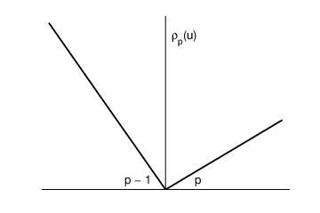
where the solution vector $\hat{\beta}_{p}$ gives the $p$ -th regression quantile and the estimated conditional quantile function is obtained as $\hat{y}=X\hat{\beta}_{p}$ . Note that the objective function (2) is such that all observations above the estimated hyperplane $X\hat{\beta}_{p}$ are weighted by $p$ , and all observations below the estimated hyperplane are weighted by $(1-p)$ . Therefore, the objective function (2) can be written as a sum of check functions or piecewise linear functions as follows,

\min_{\beta_{p}\in\mathbf{R}^{k}}\sum_{i=1}^{n}\rho_{p}(y_{i}-x^{\prime}_{i}\beta_{p}),

where $\rho_{p}(u)=u\cdot(p-I(u<0))$ and $I(\cdot)$ is an indicator function, which equals 1 if the condition inside the parenthesis is true and 0 otherwise. It is obvious from Figure 1 that the check function is not differentiable at the origin and consequently, classical methods rely upon computational techniques such as the simplex algorithm, the interior point algorithm or the smoothing algorithm (Madsen and Nielsen 1993; Chen 2007). Simulation methods, such as metaheuristic algorithms, can also be used to estimate quantile regression models (Rahman 2013).

The Bayesian method of estimating quantile regression uses the fact that maximization of the likelihood, where the error follows an AL distribution, is equivalent to minimization of the quantile objective function (Yu and Moyeed 2001). The error $\epsilon_{i}$ follows a skewed AL distribution, denoted $\epsilon_{i}\sim AL(0,1,p)$ , if the probability density function (pdf) is given by:

f_{p}(\epsilon_{i})=p(1-p)\left\{\begin{array}[]{ll}\exp(-\epsilon_{i}\,(p-1))&\mathrm{if\;\epsilon_{i}<0}\\ \exp(-\epsilon_{i}\,p)&\mathrm{if\;\epsilon_{i}\geq 0},\end{array}\right.

(3)

where the location, scale and skewness parameters equal 0, 1, and $p$ , respectively (Kotz et al. 2001; Yu and Zhang 2005). The mean and variance of $\epsilon_{i}$ with pdf (3) are as follows,

E(\epsilon_{i})=\frac{1-2p}{p(1-p)}\quad\textrm{and}\quad V(\epsilon_{i})=\frac{1-2p+2p^{2}}{p^{2}(1-p)^{2}}.

Both mean and variance, as shown above, depend on the skewness parameter $p$ , but are fixed for a given value of $p$ . Interestingly, $p$ also defines the quantile of an AL distribution and the $p$ -th quantile is always zero. This feature becomes useful in quantile regression, since estimation of a model at different quantiles simply requires a change in the value of $p$ .

Given the likelihood based on the AL distribution, the posterior distribution is proportional to the product of the likelihood and the prior distribution of the parameters. Unfortunately, the joint posterior distribution does not have a known tractable form and typically requires MCMC methods for posterior inferences. In this context, Kozumi and Kobayashi 2011 show that Gibbs sampling can be employed provided the AL distribution is represented as a mixture of normal-exponential distributions, i.e.

\epsilon_{i}=\theta w_{i}+\tau\sqrt{w_{i}}\,u_{i},\hskip 54.2025pt\forall\;i=1,\cdots,n,

(4)

where $w_{i}$ and $u_{i}$ are mutually independent, $u_{i}\sim N(0,1)$ , $w_{i}\sim\mathcal{E}(1)$ , and $\mathcal{E}$ represents an exponential distribution. The constants ( $\theta,\tau$ ) in equation (4) are defined as follows,

\theta=\frac{1-2p}{p(1-p)}\qquad\mathrm{and}\qquad\tau=\sqrt{\frac{2}{p(1-p)}}.

The normal-exponential mixture representation of the AL distribution offers access to properties of the normal distribution, which are exploited in the current paper to derive the sampler for quantile regression in ordinal models.

0.3 Quantile Regression in Ordinal Models

Ordinal models arise when the dependent (response) variable is discrete and outcomes are inherently ordered or ranked with the characteristic that scores assigned to outcomes have an ordinal meaning, but no cardinal interpretation. For example, in a survey regarding the performance of the economy, responses may be recorded as follows: 1 for ‘bad’, 2 for ‘average’ and 3 for ‘good’. The responses in such a case have ordinal meaning but no cardinal interpretation, so one cannot say a score of 2 is twice as good as a score of 1. The ordinal ranking of the responses differentiates these data from unordered choice outcomes.

A quantile regression ordinal model can be represented using a continuous latent random variable $z_{i}$ as,

z_{i}=x^{\prime}_{i}\beta_{p}+\epsilon_{i},\hskip 54.2025pt\forall\;i=1,\cdots,n,

(5)

where $x_{i}$ is a $k\times 1$ vector of covariates, $\beta_{p}$ is a $k\times 1$ vector of unknown parameters at the $p$ -th quantile, $\epsilon_{i}$ follows an AL distribution with pdf (3) and $n$ denotes the number of observations. However, the variable $z_{i}$ is unobserved and relates to the observed discrete response $y_{i}$ , which has J categories or outcomes, via the cut-point vector $\gamma_{p}$ as follows:

\gamma_{p,j-1}<z_{i}\leq\gamma_{p,j}\;\Rightarrow\;\emph{y_{i}=j},\hskip 54.2025pt\forall\;i=1,\cdots,n;\;j=1,\cdots,J,

(6)

where $\gamma_{p,0}=-\infty$ and $\gamma_{p,J}=\infty$ . In addition, $\gamma_{p,1}$ is typically set to 0, which anchors the location of the distribution required for parameter identification (see Jeliazkov et al. 2008). Given the data vector $y$ = $(y_{1},\cdots,y_{n})^{\prime}$ , the likelihood for the model expressed as a function of unknown parameters $(\beta_{p},\gamma_{p})$ can be written as,

\begin{split}f(\beta_{p},\gamma_{p};y)&=\prod_{i=1}^{n}\prod_{j=1}^{J}P(y_{i}=j|\beta_{p},\gamma_{p})^{I(y_{i}=j)}\\ &=\prod_{i=1}^{n}\prod_{j=1}^{J}\bigg[F_{AL}(\gamma_{p,j}-x^{\prime}_{i}\beta_{p})-F_{AL}(\gamma_{p,j-1}-x^{\prime}_{i}\beta_{p})\bigg]^{I(y_{i}=j)}\end{split}

(7)

where, $F_{AL}(\cdot)$ denotes the cumulative distribution function (cdf) of an AL distribution and $I(y_{i}=j)$ is an indicator function, which equals 1 if $y_{i}=j$ and 0 otherwise.

The Bayesian approach to estimating quantile ordinal models utilizes the latent variable representation (5) together with the normal-exponential representation (4) of the AL distribution. The $p$ -th quantile ordinal model can therefore be expressed as,

z_{i}=x^{\prime}_{i}\beta_{p}+\theta w_{i}+\tau\sqrt{w_{i}}\,u_{i},\hskip 36.135pt\forall\;i=1,\cdots,n.

(8)

It is clear from formulation (8) that the latent variable $z_{i}|\beta_{p},w_{i}\sim N(x^{\prime}_{i}\beta_{p}+\theta w_{i},\tau^{2}w_{i})$ , allowing usage of the convenient properties of normal distribution in the estimation procedure.

Before moving forward, it is beneficial to subdivide ordinal models, as $\mathrm{OR_{I}}$ and $\mathrm{OR_{II}}$ , based on the number of outcomes and the type of scale restriction employed. The subdivision is employed to present two algorithms — a general algorithm for estimation of ordinal models that utilizes Gibbs sampling and the Metropolis-Hastings (MH) algorithm, and a simpler algorithm for estimation of ordinal models with three outcomes that solely relies on Gibbs sampling. They form the subject of discussion in the next two subsections.

On a side note, although the derivation of posterior distributions for $\mathrm{OR_{I}}$ and $\mathrm{OR_{II}}$ models utilize a normal prior on $\beta_{p}$ , it is not the default choice. One may also employ the normal-exponential mixture representation of the Laplace or double exponential distribution as the prior distribution (Andrews and Mallows 1974; Park and Casella 2008; Kozumi and Kobayashi 2011). The full conditional posteriors with a Laplace prior is a straightforward modification of the derivations with a normal prior, and hence has not been presented to keep the paper within reasonable length.

0.3.1 $\mathrm{OR_{I}}$ Model

The term “ $\mathrm{OR_{I}}$ model,” as used in the paper, refers to an ordinal model (equations (8) and (6)) in which the number of outcomes is greater than three ( $J>3$ ), location restriction is achieved via $\gamma_{p,1}=0$ and scale restriction is enforced via fixed variance (since $V(\epsilon_{i})$ is constant for a given $p$ ). The location restriction removes the possibility of shifting the distribution without changing the probability of observing $y_{i}$ and the scale restriction fixes the scale of the latent data that is implied by the cdf of the AL distribution, i.e., $F_{AL}$ . Note that one may incorporate $J=3$ outcomes within the definition of $\mathrm{OR_{I}}$ model, but estimation would involve the MH algorithm, which can be avoided as presented in Section 0.3.2.

Estimation

Estimation of the $\mathrm{OR_{I}}$ model utilizes the approach of Kozumi and Kobayashi 2011 with the addition of the following two components: first, location and scale restrictions, and second, threshold or cut-point vector $\gamma_{p}$ . The location and scale restrictions are easy to impose, but sampling of the cut-points requires additional consideration. In particular, two issues arise with respect to the sampling of $\gamma_{p}$ : the ordering constraints and the absence of a known conditional distribution of the transformed cut-points.

The ordering constraints within the cut-point vector $\gamma_{p}$ cause complication since it is difficult to satisfy the ordering during sampling. Ordering can be removed by using any monotone transformation from a compact set to the real line. The paper employs the logarithmic transformation,

\delta_{p,j}=\ln(\gamma_{p,j}-\gamma_{p,j-1}),\qquad 2\leq j\leq J-1.

(9)

Other transformations, such as log-ratios of category bin-widths or trigonometric functions like arctan and arcsin, are also possible. The original cut-points can then be obtained by a one-to-one mapping between $\delta_{p}=(\delta_{p,2},\cdots,\delta_{p,J-1})^{\prime}$ and $\gamma_{p}=(\gamma_{p,1},\gamma_{p,2},\allowbreak{\cdots,\gamma_{p,J-1}})^{\prime}$ where $\gamma_{p,1}=0$ and recall that the first cut-point $\gamma_{p,0}=-\infty$ and the last cut-point $\gamma_{p,J}=\infty$ .

The transformed cut-point vector $\delta_{p}$ does not have a known conditional distribution and is sampled using an MH algorithm with a random-walk proposal density. A tailored MH algorithm, as done in Jeliazkov et al. 2008, was attempted but later aborted because of the increased computational time due to maximization of the likelihood function at each iteration. However, estimates obtained from both forms of the MH algorithm are identical.

Once the difficulties related to the cut-points have been addressed, the joint posterior distribution can be derived using the Bayes’ theorem. The joint posterior distribution for $\beta_{p},\delta_{p}$ , latent weight $w$ and latent data $z$ , assuming the following independent normal priors,

	$\displaystyle\beta_{p}$	$\displaystyle\sim N(\beta_{p0},B_{p0}),\hskip 36.135pt\mathrm{and}$
	$\displaystyle\delta_{p}$	$\displaystyle\sim N(\delta_{p0},D_{p0}),$

can be written as proportional to the product of the likelihood and the priors as,

$\displaystyle\pi(z,\beta_{p},\delta_{p},w\|y)$	$\displaystyle\propto f(y\|z,\beta_{p},\delta_{p},w)\;\pi(z,\beta_{p},\delta_{p}\|w)\;\pi(w)$
	$\displaystyle\propto f(y\|z,\beta_{p},\delta_{p},w)\;\pi(z\|\beta_{p},w)\;\pi(\beta_{p},\delta_{p})\;\pi(w)$	(10)
	$\displaystyle\propto\Big\{\prod_{i=1}^{n}f(y_{i}\|z_{i},\delta_{p})\Big\}\;\pi(z\|\beta_{p},w)\;\pi(w)\;\pi(\beta_{p})\;\pi(\delta_{p}),$

where the likelihood, based on $AL(0,1,p)$ , uses the fact that given the latent variable $z$ and the cut-points $\delta_{p}$ , the observed $y_{i}$ is independent of $\beta_{p}$ because (6) determines $y_{i}$ given $(z_{i},\delta_{p})$ with probability one and that relation is not dependent on $\beta_{p}$ . In the second line, the density $\pi(z|\beta_{p},w)$ can be obtained from (8) and is given by $\pi(z|\beta_{p},w)=\prod_{i=1}^{n}N(z_{i}|x^{\prime}_{i}\beta_{p}+\theta w_{i},\tau^{2}w_{i})$ . The last line in equation (10) uses prior independence between $\beta_{p}$ and $\delta_{p}$ . With the help of preceding explanations, the “complete data” posterior in equation (10) can be written as,

	$\displaystyle\pi(z,\beta_{p},\delta_{p},w\|y)$	$\displaystyle\propto\bigg\{\prod_{i=1}^{n}1\{\gamma_{p,y_{i}-1}<z_{i}\leq\gamma_{p,y_{i}}\}\;N(z_{i}\|x^{\prime}_{i}\beta_{p}+\theta w_{i},\tau^{2}w_{i})\;\mathcal{E}(w_{i}\|1)\bigg\}$
		$\displaystyle\qquad\times N(\beta_{p0},B_{p0})\;N(\delta_{p0},D_{p0}).$		(11)

Using equation (11) and two identification constraints, $\gamma_{p,1}=0$ and $V(\epsilon)=\frac{1-2p+2p^{2}}{p^{2}(1-p)^{2}}$ (fixed for a given $p$ ), the objects of interest $(z,\beta_{p},\delta_{p},w)$ can be sampled as presented in Algorithm 1.

Algorithm 1 (Sampling in $\mathrm{OR_{I}}$ model)

•

Sample $\beta_{p}|z,w$ $\sim$ $N(\tilde{\beta}_{p},\tilde{B}_{p})$ , where,
$\tilde{B}^{-1}_{p}=\bigg(\sum_{i=1}^{n}\frac{x_{i}x^{\prime}_{i}}{\tau^{2}w_{i}}+B_{p0}^{-1}\bigg)$ and $\tilde{\beta}_{p}=\tilde{B}_{p}\bigg(\sum_{i=1}^{n}\frac{x_{i}(z_{i}-\theta w_{i})}{\tau^{2}w_{i}}+B_{p0}^{-1}\beta_{p0}\bigg)$ .
•

Sample $w_{i}|\beta_{p},z_{i}$ $\sim$ $GIG\,(0.5,\tilde{\lambda}_{i},\tilde{\eta})$ , for $i=1,\cdots,n$ , where,
$\tilde{\lambda}_{i}=\Big(\frac{z_{i}-x^{\prime}_{i}\beta_{p}}{\tau}\Big)^{2}$ and $\tilde{\eta}=\Big(\frac{\theta^{2}}{\tau^{2}}+2\Big)$ .

•

Sample $\delta_{p}|y,\beta_{p}$ marginally of $w$ (latent weight) and $z$ (latent data), by generating $\delta_{p}^{\prime}$ using a random-walk chain $\delta^{\prime}_{p}=\delta_{p}+u$ , where $u\sim N(0_{J-2},\iota^{2}\hat{D})$ , $\iota$ is a tuning parameter and $\hat{D}$ denotes negative inverse Hessian, obtained by maximizing the log-likelihood with respect to $\delta_{p}$ . Given the current value of $\delta_{p}$ and the proposed draw $\delta^{\prime}_{p}$ , return $\delta^{\prime}_{p}$ with probability,

\alpha_{MH}(\delta_{p},\delta^{\prime}_{p})=\min\bigg\{1,\frac{\;f(y|\beta_{p},\delta^{\prime}_{p})\;\pi(\beta_{p},\delta^{\prime}_{p})}{f(y|\beta_{p},\delta_{p})\;\pi(\beta_{p},\delta_{p})}\bigg\};

otherwise repeat the old value $\delta_{p}$ . The variance of $u$ may be tuned as needed for appropriate step size and acceptance rate.

•

Sample $z_{i}|y,\beta_{p},\gamma_{p},w$ $\sim$ $TN_{(\gamma_{p,j-1},\gamma_{p,j})}(x^{\prime}_{i}\beta_{p}+\theta w_{i},\tau^{2}w_{i})$ for $i=1,\cdots,n$ , where $\gamma_{p}$ is obtained by one-to-one mapping between $\gamma_{p}$ and $\delta_{p}$ from equation (9).

The sampling algorithm for $\mathrm{OR_{I}}$ model is fairly straightforward and primarily involves drawing parameters, with the exception of $\delta_{p}$ , from their conditional distributions. The parameter $\beta_{p}$ conditional on $z$ and $w$ follows a normal distribution, draws from which are a routine exercise in econometrics. On the other hand, the conditional distribution of latent weight $w$ follows a Generalized Inverse Gaussian (GIG) distribution, draws from which can be obtained either by the ratio of uniforms method (Dagpunar 1988; Dagpunar 1989) or the envelope rejection method (Dagpunar 2007). The transformed cut-point vector $\delta_{p}$ , as mentioned earlier, does not have a known conditional distribution and is sampled using the MH algorithm, marginally of $(z,w)$ because the full likelihood (7) conditional on $(\beta_{p},\delta_{p})$ is independent of $(z,w)$ . Sampling of cut-points from the full likelihood was also employed in Jeliazkov et al. 2008. Finally, the latent variable $z$ conditional on $(y,\beta_{p},\gamma_{p},w)$ is sampled from a truncated normal distribution, where the region of truncation is determined based on a one-to-one mapping from $\delta_{p}$ using equation (9). The derivations of the full conditional distributions of ( $\beta_{p},w,z$ ) and details on the MH sampling of the cut-point vector $\delta_{p}$ are presented in Appendix F.

The $\mathrm{OR_{I}}$ model can also be estimated using an alternative identification scheme where the scale restriction is enforced by fixing a second cut-point, for example $\gamma_{p,2}=1$ . Fixing a second cut-point would introduce the scale parameter $\sigma_{p}$ into the model (8) and consequently, add another sampling block in Algorithm 1. This identification scheme, although plausible, seems unnecessary for the $\mathrm{OR_{I}}$ model and may lead to higher inefficiency factors; however, it can be gainfully utilized when number of outcomes equals 3 and is described in Section 0.3.2.

Simulation Study

A simulation study was carried out to examine the performance of the algorithm proposed in Section 0.3.1 and compare model fit with the ordinal probit model (see Algorithm 2 in Jeliazkov et al. 2008). In particular, 300 observations were generated from the model $z_{i}=x^{\prime}_{i}\beta+\epsilon_{i}$ , with $\beta$ = $(-2\;3\;4)^{\prime}$ , covariates were generated from standard uniform distributions, and $\epsilon$ was generated from a mixture of logistic distributions, $\mathcal{L}(-5,\pi^{2}/3)$ and $\mathcal{L}(2,\pi^{2}/3)$ , with mix proportions 0.3 and 0.7, respectively. The histogram of the continuous variable $z$ (not shown) was approximately unimodal and negatively skewed. The discrete response variable $y$ was constructed based on the cut-point vector $\gamma=(0,2,3)$ . In the simulated data, the number of observations corresponding to the four categories of $y$ were 107, 43, 36 and 114, respectively.

	25th quantile			50th quantile			75th quantile			ord probit
parameters	mean	std	if	mean	std	if	mean	std	if	mean	std	if
$\beta_{1}$	$-1.62$	$0.39$	$2.25$	$-0.75$	$0.31$	$1.95$	$0.10$	$0.36$	$2.27$	$-0.70$	$0.18$	$1.22$
$\beta_{2}$	$1.20$	$0.50$	$2.13$	$1.64$	$0.42$	$2.02$	$2.44$	$0.49$	$2.66$	$1.08$	$0.22$	$1.21$
$\beta_{3}$	$1.12$	$0.51$	$2.00$	$1.96$	$0.45$	$2.29$	$2.97$	$0.50$	$2.58$	$1.22$	$0.23$	$1.23$
$\delta_{1}$	$0.01$	$0.15$	$2.36$	$-0.22$	$0.15$	$3.11$	$0.23$	$0.15$	$4.54$	$-0.86$	$0.13$	$2.66$
$\delta_{2}$	$0.07$	$0.16$	$2.19$	$-0.34$	$0.15$	$2.59$	$-0.09$	$0.16$	$3.43$	$-0.97$	$0.14$	$2.33$

Table 1: Posterior mean (mean), standard deviation (std) and inefficiency factor (if) of the parameters in the 25th, 50th and 75th quantile ordinal models and ordinal probit model.

The posterior estimates for the model parameters were obtained based on the simulated data and the following independent normal priors: $\beta_{p}\sim N(0_{3},I_{3})$ and $\delta_{p}\sim N(0_{2},0.25\,I_{2})$ , for $p=(0.25,0.5,0.75)$ . The same priors were utilized in the estimation of the ordinal probit model. Use of less informative priors only causes a minor change in the posterior estimates. Table 1 reports the MCMC results obtained from 12,000 iterations, after a burn-in of 3,000 iterations, along with the inefficiency factors calculated using the batch-means method (see Greenberg 2012). MH acceptance rate for $\delta_{p}$ was around 30% for all values of $p$ and $\iota=\sqrt{3}$ . Convergence of MCMC draws, as observed from the trace plots (not shown), was quick and occurred within a few hundred iterations. The sampling took approximately 120 and 50 seconds per $1,000$ iterations for the quantile and ordinal probit models, respectively.

The quantile ordinal models offer several choice of quantiles and one may interpret the various choices of $p$ as corresponding to different family of link functions. In such a scenario, model selection criterion such as deviance information criterion or DIC (Spiegelhalter et al. 2002; Celeux et al. 2006) may be utilized to choose a value of $p$ that is most consistent with the data. To illustrate, DIC was computed for the 25th, 50th and 75th quantile models and the numbers were $755.67$ , $721.81$ and $704.16$ , respectively. The DIC for the ordinal probit model was $721.56$ . Hence, amongst all the models considered, the 75th quantile model provides the best fit, which is correct since the distribution of the continuous variable $z$ is negatively skewed and so is the AL distribution for $p=0.75$ . The median quantile model and ordinal probit model give almost identical DICs, but both provide a poorer fit compared to the 75th quantile model.

0.3.2 $\mathrm{OR_{II}}$ Model

The term “ $\mathrm{OR_{II}}$ model,” as used in the paper, refers to an ordinal model in which the number of outcomes equals three ( $J=3$ ), and both location and scale restrictions are achieved through fixing cut-points. In this case, fixing a second cut-point simplifies the sampling procedure, since with three outcomes there are only two cut-points, both of which are known by virtue of being fixed, so $\gamma_{p}=\gamma$ for all $p$ . However, use of this identification scheme introduces a scale parameter in the model (8) that needs to be estimated. The $\mathrm{OR_{II}}$ model can be written as follows,

\begin{split}&z_{i}=x^{\prime}_{i}\beta_{p}+\sigma_{p}\epsilon_{i}=x^{\prime}_{i}\beta_{p}+\sigma_{p}\theta w_{i}+\sigma_{p}\tau\sqrt{w_{i}}\,u_{i},\hskip 79.49744pt\forall\;i=1,\cdots,n,\\ &\gamma_{j-1}<z_{i}\leq\gamma_{j}\;\Rightarrow\;\emph{$y_{i}$=j},\hskip 122.85876pt\forall\;i=1,\cdots,n;\;j=1,2,3,\end{split}

(12)

where $\sigma_{p}$ is the scale parameter at quantile $p$ and ( $\gamma_{1},\gamma_{2}$ ) are fixed at some values, in addition to $\gamma_{0}=-\infty$ and $\gamma_{3}=\infty$ . Note that the scale parameter will be dependent on $p$ because it will adjust to capture the variability in the data, since $V(\epsilon)$ is constant for a given $p$ .

Estimation

Estimation of the $\mathrm{OR_{II}}$ model (12), although free of the MH algorithm, cannot directly utilize Gibbs sampling since the conditional mean of $z_{i}|\beta_{p},w_{i}$ involves the scale parameter $\sigma_{p}$ (Kozumi and Kobayashi 2011). However, the scale parameter $\sigma_{p}$ can be removed from the conditional mean through a simple reformulation as follows,

z_{i}=x^{\prime}_{i}\beta_{p}+\theta\nu_{i}+\tau\sqrt{\sigma_{p}\nu_{i}}\,u_{i},

(13)

where $\nu_{i}=\sigma_{p}w_{i}$ and consequently, $z_{i}|\beta_{p},\sigma_{p},\nu_{i}\sim N(x^{\prime}_{i}\beta_{p}+\theta\nu_{i},\tau^{2}\sigma_{p}\nu_{i})$ . In the current formulation (13), the $\mathrm{OR_{II}}$ model becomes conducive to Gibbs sampling. The next step relates to prior distributions and they were specified as,

	$\displaystyle\beta_{p}$	$\displaystyle\sim N(\beta_{p0},B_{p0}),$
	$\displaystyle\sigma_{p}$	$\displaystyle\sim IG(n_{0}/2,d_{0}/2),$
	$\displaystyle\nu_{i}$	$\displaystyle\sim\mathcal{E}(\sigma_{p}),$

where $IG$ and $\mathcal{E}$ stand for inverse-gamma and exponential distributions, respectively. Employing Bayes’ theorem, the joint posterior distribution for ( $z,\beta_{p},\nu,\sigma_{p}$ ) can be written as proportional to the product of the likelihood and the priors,

\begin{split}\pi(z,\beta_{p},\nu,\sigma_{p}|y)&\propto f(y|z,\beta_{p},\nu,\sigma_{p})\;\pi(z|\beta_{p},\nu,\sigma_{p})\;\pi(\nu|\sigma_{p})\;\pi(\beta_{p})\;\pi(\sigma_{p}),\\ &\propto\Big\{\prod_{i=1}^{n}f(y_{i}|z_{i},\sigma_{p})\Big\}\;\pi(z|\beta_{p},\nu,\sigma_{p})\;\pi(\nu|\sigma_{p})\;\pi(\beta_{p})\;\pi(\sigma_{p}),\end{split}

(14)

where the likelihood uses the property that $\sigma_{p}\,\epsilon\sim AL(0,\sigma_{p},p)$ and given the known cut-points and latent data $z$ , the observed $y_{i}$ does not depend on ( $\beta_{p},\nu$ ). The conditional distribution of the latent data $z$ can be obtained from (13) as $\pi(z|\beta_{p},\sigma_{p},\nu)=\prod_{i=1}^{n}N(x^{\prime}_{i}\beta_{p}+\theta\nu_{i},\tau^{2}\sigma_{p}\nu_{i})$ . Combining the likelihood, conditional distribution of $z$ and the priors, the “complete data” posterior in (14) can be expressed as,

	$\displaystyle\pi(z,\beta_{p},\nu,\sigma_{p}\|y)$	$\displaystyle\propto\bigg\{\prod_{i=1}^{n}1\{\gamma_{y_{i}-1}<z_{i}\leq\gamma_{y_{i}}\}\;N(z_{i}\|x^{\prime}_{i}\beta_{p}+\theta\nu_{i},\tau^{2}\sigma_{p}\nu_{i})\;\mathcal{E}(\nu_{i}\|\sigma_{p})\bigg\}$
		$\displaystyle\qquad\times N(\beta_{p0},B_{p0})\;IG(n_{0}/2,d_{0}/2),$		(15)

which can be utilized to derive the full conditional distributions for all parameters of interest namely, $\beta_{p}$ , $\nu$ and $\sigma_{p}$ . The derivations, presented in Appendix G, require collecting terms for a parameter of interest assuming other parameters are known and then identifying the distribution for the parameter of interest. Following this intuitively simple approach, the parameters can be sampled from their conditional posteriors as presented in Algorithm 2.

Algorithm 2 (Sampling in $\mathrm{OR_{II}}$ model)

•

Sample $\beta_{p}|z,\sigma_{p},\nu$ $\sim$ $N(\tilde{\beta}_{p},\tilde{B}_{p})$ , where,
$\tilde{B}^{-1}_{p}=\bigg(\sum_{i=1}^{n}\frac{x_{i}x^{\prime}_{i}}{\tau^{2}\sigma_{p}\nu_{i}}+B_{p0}^{-1}\bigg)$ and $\tilde{\beta}_{p}=\tilde{B}_{p}\bigg(\sum_{i=1}^{n}\frac{x_{i}(z_{i}-\theta\nu_{i})}{\tau^{2}\sigma_{p}\nu_{i}}+B_{p0}^{-1}\beta_{p0}\bigg)$ .
•

Sample $\sigma_{p}|z,\beta_{p},\nu$ $\sim$ $IG(\tilde{n}/2,\tilde{d}/2)$ , where,
$\tilde{n}=(n_{0}+3n)$ and $\tilde{d}=\sum_{i=1}^{n}(z_{i}-x^{\prime}_{i}\beta_{p}-\theta\nu_{i})^{2}/\tau^{2}\nu_{i}+d_{0}+2\sum_{i=1}^{n}\nu_{i}$ .
•

Sample $\nu_{i}|z_{i},\beta_{p},\sigma_{p}$ $\sim$ $GIG(0.5,\tilde{\lambda_{i}},\tilde{\eta})$ , for $i=1,\cdots,n$ , where,
$\tilde{\lambda_{i}}=\frac{(z_{i}-x^{\prime}_{i}\beta_{p})^{2}}{\tau^{2}\sigma_{p}}$ and $\tilde{\eta}=\Big(\frac{\theta^{2}}{\tau^{2}\sigma_{p}}+\frac{2}{\sigma_{p}}\Big)$ .
•

Sample $z_{i}|y,\beta_{p},\sigma_{p},\nu_{i}$ $\sim$ $TN_{(\gamma_{j-1},\gamma_{j})}(x^{\prime}_{i}\beta_{p}+\theta\nu_{i},\tau^{2}\sigma_{p}\nu_{i})$ for $i=1,\cdots,n$ , and $j=1,2,3$ .

Simulation Study

A simulation study was carried out to examine the performance of the algorithm proposed in Section 0.3.2 and compare model fit with the ordinal probit model (see Algorithm 3 in Jeliazkov et al. 2008). In particular, 300 observations were generated from the model $z_{i}=x^{\prime}_{i}\beta+\epsilon_{i}$ , with $\beta$ = $(2\;2\;1)^{\prime}$ , covariates were generated from a standard bivariate normal distribution with correlation 0.25 and $\epsilon$ was generated from a mixture of Gaussian distributions, $N(-6,4)$ and $N(5,1)$ , with mix proportions 0.3 and 0.7, respectively. The histogram of continuous variable $z$ (not shown) was bimodal and negatively skewed. The discrete response variable $y$ was constructed based on cut-point vector $\gamma$ = ( $0$ , $4$ ). In the simulated data, the number of observations corresponding to the three category of $y$ were 77, 38 and 185, respectively.

The posterior estimates in the quantile ordinal models were obtained based on the following priors: $\beta_{p}\sim N(0_{3},I_{3})$ , $\sigma_{p}\sim IG(5/2,8/2)$ and $\nu\sim\mathcal{E}(\sigma_{p})$ for $p=(0.25,0.5,0.75)$ . Posterior estimation of ordinal probit model used the same prior on $\beta$ and $\sigma^{2}\sim IG(5/2,8/2)$ . The hyperparameters of the inverse-gamma distribution was chosen to keep the prior less informative. For all the models, the cut-points were fixed at ( $0$ , $4$ ), which are same as that used to construct the discrete response $y$ . Table 2 reports the Gibbs sampling results obtained from 12,000 iterations after a burn-in of 3,000 iterations, along with the inefficiency factors calculated using the batch-means method (see Greenberg 2012). Convergence of MCMC draws, as observed from the trace plots (not shown), occurred within a few hundred iterations. The sampling procedure took approximately 87 and 75 seconds per 1,000 iterations for the quantile and ordinal probit models, respectively.

parameters	mean	std	if	mean	std	if	mean	std	if	mean	std	if
	25th quantile			50th quantile			75th quantile			ord probit
$\beta_{1}$	$0.27$	$0.58$	$2.12$	$5.03$	$0.41$	$2.31$	$7.05$	$0.37$	$5.47$	$4.62$	$0.49$	$1.28$
$\beta_{2}$	$1.70$	$0.57$	$1.96$	$1.63$	$0.39$	$2.10$	$1.67$	$0.31$	$4.50$	$2.05$	$0.49$	$1.29$
$\beta_{3}$	$0.41$	$0.57$	$1.88$	$0.64$	$0.41$	$2.04$	$0.70$	$0.30$	$3.14$	$0.68$	$0.50$	$1.21$
$\sigma$	$4.03$	$0.60$	$4.42$	$3.28$	$0.43$	$3.95$	$1.41$	$0.15$	$4.11$	$7.79$	$0.95$	$3.41$

Table 2: Posterior mean (mean), standard deviation (std) and inefficiency factor (if) of the parameters in the 25th, 50th and 75th quantile ordinal models and ordinal probit model.

In order to compare the 25th, 50th, 75th quantile models and the ordinal probit model, the DIC was computed and the values were $540.61$ , $528.96$ , $526.19$ and $533.80$ , respectively. Therefore, amongst the quantile models, the 75th quantile model provides the best fit, which is correct since the distribution of the continuous variable $z$ is negatively skewed and so is the AL distribution for $p=0.75$ . In addition, both the 50th and 75th quantile models provide a better fit than the ordinal probit model.

0.4 Application

In this section, the proposed algorithms for quantile estimation of ordinal models are used in two applications that are of interest in economics and the broader social sciences. The first application uses the National Longitudinal Study of Youth (NLSY, 1979) survey data from Jeliazkov et al. 2008 to analyze the topic of educational attainment and extends the analysis to the domain of quantile regression. The second application uses the American National Election Studies (ANES) survey data to evaluate public opinion on raising federal income taxes for individuals’ who make more than $250,000 per year.

0.4.1 Educational Attainment

In this application, the NLSY data taken from Jeliazkov et al. 2008 was utilized to study educational attainment. The NLSY was started in 1979 with more than 12,000 youths to conduct annual interviews on a wide range of demographic questions. However, the sample used by Jeliazkov et al. 2008 contains data on 3923 individuals only, because the analysis was restricted to cohorts aged 14-17 in 1979 and for whom family income variable could be constructed.

parameters	mean	std	mean	std	mean	std	mean	std
	25th quantile		50th quantile		75th quantile		ord probit
intercept	$-5.92$	$0.33$	$-3.18$	$0.22$	$-0.61$	$0.27$	$-1.34$	$0.09$
family income (sq. rt.)	$0.39$	$0.04$	$0.28$	$0.02$	$0.28$	$0.03$	$0.14$	$0.01$
mother’s education	$0.18$	$0.03$	$0.12$	$0.02$	$0.12$	$0.02$	$0.05$	$0.01$
father’s education	$0.21$	$0.02$	$0.18$	$0.02$	$0.17$	$0.02$	$0.07$	$0.01$
mother worked	$0.08$	$0.10$	$0.07$	$0.08$	$0.06$	$0.10$	$0.03$	$0.04$
female	$0.58$	$0.10$	$0.35$	$0.08$	$0.23$	$0.09$	$0.16$	$0.04$
black	$0.64$	$0.13$	$0.43$	$0.09$	$0.25$	$0.11$	$0.15$	$0.04$
urban	$-0.42$	$0.14$	$-0.08$	$0.09$	$0.13$	$0.11$	$-0.05$	$0.04$
south	$0.13$	$0.13$	$0.08$	$0.08$	$0.15$	$0.10$	$0.05$	$0.04$
age cohort 2	$-0.09$	$0.23$	$-0.05$	$0.12$	$-0.03$	$0.14$	$-0.03$	$0.05$
age cohort 3	$-0.06$	$0.16$	$-0.05$	$0.12$	$0.04$	$0.15$	$0.00$	$0.05$
age cohort 4	$0.50$	$0.16$	$0.49$	$0.13$	$0.54$	$0.15$	$0.23$	$0.06$
$\delta_{1}$	$1.11$	$0.03$	$0.90$	$0.03$	$1.27$	$0.03$	$0.08$	$0.02$
$\delta_{2}$	$1.13$	$0.03$	$0.55$	$0.03$	$0.56$	$0.03$	$-0.28$	$0.03$

Table 3: Posterior mean (mean) and standard deviation (std) of model parameters in the educational attainment application. Identification achieved through variance restriction.

The dependent variable in the model, education degrees, has four categories: (i) less than high school, (ii) high school degree, (iii) some college or associate’s degree, and (iv) college or graduate degree, and the number of observations corresponding to each category are 897 (22.87%), 1392 (35.48%), 876 (22.33%) and 758 (19.32%), respectively. The independent variables included in the model are as follows: square root of family income, mother’s education, father’s education, mother’s working status, gender, race, and whether the youth lived in an urban area or the South at the age of 14. In addition, to control for age cohort effects, three indicator variables were included to indicate an individuals’ age in 1979. Using data on the above variables, the application studies the effect of family background, individual and school variables on educational attainment.

In this application, there are four outcomes and hence the fixed variance restriction was utilized to estimate the quantile models (using the $\mathrm{OR_{I}}$ framework) and the ordinal probit model. Priors on the parameters were same as that in the simulation study of Section 0.3.1. Table 3 reports the results obtained from 12,000 iterations after a burn-in of 3,000 iterations. Inefficiency factors, not reported, were less than 6 for all the parameters and MCMC simulation draws converged to the target distribution within a few hundred iterations.

The results for the ordinal probit model ( $\epsilon\sim N(0,I)$ ), presented in the last two columns of Table 3, are identical to that obtained by Jeliazkov et al. 2008. It is seen that the signs of the coefficients are mostly consistent with what is typically found in the literature. For example, parental education and higher family income have a positive effect on educational attainment. Similarly, mother’s labor force participation has a positive effect on educational attainment. The table also shows that conditional on other covariates, females, blacks or individuals’ from South have higher educational attainment, respective to the base categories. On the other hand, living in an urban area has a negative effect on educational attainment and the age cohort variables have a different effect on the educational attainment of an individual.

To supplement the analysis, Table 3 also presents the posterior estimates and standard deviations of the parameters for the ordinal quantile regression model ( $\epsilon\sim AL(0,1\allowbreak{,p)}$ ), estimated for $p=0.25,0.50$ , and $0.75$ . It is seen that the sign and magnitude of the estimates for the quantile models are somewhat similar to that obtained for the ordinal probit model. However, this does not imply similar inferences, as explained in the next paragraph. The last two rows of Table 3, present the posterior mean and standard deviation of the transformed cut-point vector $\delta_{p}=(\delta_{1,p},\delta_{2,p})^{\prime}$ . Clearly, the estimated $\delta$ for the ordinal probit model is different compared to the quantile regression models. This difference is related to different distributional assumptions associated with the models.

	25th quantile	50th quantile	75th quantile	ord probit
$\Delta$ P(high school dropout)	$-0.0415$	$-0.0313$	$-0.0193$	$-0.0390$
$\Delta$ P(high school degree)	$\phantom{+}0.0022$	$-0.0133$	$-0.0186$	$-0.0000$
$\Delta$ P(college or associate’s)	$\phantom{+}0.0204$	$\phantom{+}0.0201$	$\phantom{+}0.0097$	$\phantom{+}0.0000$
$\Delta$ P(college or graduate)	$\phantom{+}0.0188$	$\phantom{+}0.0246$	$\phantom{+}0.0282$	$\phantom{+}0.0390$

Table 4: Change in predicted probabilities for a $10,000 increase in income.

In addition to the above analysis, it is necessary to emphasize that the link functions associated with ordinal probit and quantile ordinal models are non-linear and non-monotonic, as such an interpretation of the resulting parameter estimates is not straightforward since the coefficients by themselves do not give the impact of a change in one or more of the covariates. Consequently, the $\beta$ estimates from the quantile models and ordinal probit model do not imply the same covariate effects. To explain and highlight the differences in covariate effects, I computed the effect of a $10,000 increase in family income on educational outcomes, marginalized over parameters and remaining covariates. The results are reported in Table 4, which shows that the change in predicted probabilities are different in ordinal probit and quantile models. For example, the $10,000 increase in income decreases the probability of high school dropout by $0.039$ in the ordinal probit model. In contrast, the same probability decreases by $0.0415$ , $0.0313$ and $0.0193$ at the 25th, 50th and 75th quantiles, respectively.

Finally, an investigation on model selection based on the DIC reports the following numbers: $9840.75$ , $9781.02$ , and $9977.30$ for the 25th, 50th and 75th quantile models, respectively. The DIC for the ordinal probit model was $9736.21$ . Hence, according to DIC the ordinal probit model provides the best fit amongst the models considered, followed by the median model. However, it may be possible that for another value of $p$ , possibly close to $p=0.50$ , the DIC is lower than the DIC for the ordinal probit model.

0.4.2 Tax Policy

This application aims to analyze public opinion on a recently considered tax policy: the proposal to raise federal income taxes for couples (individuals) earning more than $250,000 ($200,000) per year (hereafter, termed “pro-growth” policy), and aims to identify factors that may increase or decrease support in favor of the proposed policy.

The pro-growth policy, proposed by President Barack H. Obama in 2010, was essentially aimed to extend the “Bush Tax” cuts for the lower and middle income class, but restore higher rates for the richer class. It thereby aimed to promote growth in the U.S. economy, struggling due to the recession, by supporting consumption amongst the low-middle income families. The policy became a subject of extended political debate with respect to the definition of benchmark income, beneficiaries of the tax cuts and whether it would spur sufficient growth. However, the proposed policy received a two-year extension and was part of a larger tax and economic package, named the “Tax Relief, Unemployment Insurance Reauthorization, and Job Creation Act of 2010”. The pro-growth policy re-surfaced in the 2012 presidential election and formed a crucial point of discussion during the presidential debate.

variables	description	mean	count
employed	Indicator for individual being employed	$0.53$	$621$
income	Indicator for household income $>\$75,000$	$0.30$	$346$
bachelors	Individual’s highest degree is Bachelors	$0.20$	$235$
post-bachelors	Highest degree is Masters, Professional or Doctorate	$0.09$	$108$
computers	Individual or household owns a computer	$0.84$	$972$
cellphone	Individual or household owns a cell phone	$0.90$	$1,051$
white	Race of the individual is white	$0.86$	$1,004$

Table 5: Variable definitions and data summary.

The pro-growth policy was included as a survey question in the 2010-2012 American National Election Studies (ANES) on the Evaluations of Government and Society Study 1 (EGSS 1). The ANES survey was conducted over the internet using nationally representative probability samples and after removing missing observations provides $1,164$ observations. The survey recorded individuals’ opinion as either oppose, neither favor nor oppose, or favor the tax increase. This forms the dependent variable in the model with 263 (22.59%), 261 (22.42%) and 640 (54.98%) observations in the respective categories. In addition, the survey collected information on a wide range of demographic variables, some of which were included as independent variables in the model. They include employment status, income level, education, computer ownership, cell phone ownership and race. Definition of the variables are presented in Table 5 together with the mean and count on each of them.

parameters	mean	std	mean	std	mean	std	mean	std
	25th quantile		50th quantile		75th quantile		ord probit
intercept	$1.00$	$0.46$	$2.10$	$0.43$	$3.42$	$0.37$	$2.58$	$0.53$
employed	$-0.04$	$0.29$	$0.20$	$0.26$	$0.21$	$0.24$	$0.16$	$0.32$
income	$-0.73$	$0.34$	$-0.46$	$0.30$	$-0.47$	$0.28$	$-0.72$	$0.37$
bachelors	$-0.17$	$0.38$	$0.07$	$0.33$	$0.12$	$0.32$	$-0.07$	$0.40$
post-bachelors	$-0.02$	$0.44$	$0.43$	$0.40$	$0.53$	$0.39$	$0.28$	$0.47$
computers	$0.02$	$0.35$	$0.62$	$0.33$	$0.61$	$0.29$	$0.53$	$0.41$
cellphone	$0.38$	$0.42$	$0.78$	$0.38$	$0.75$	$0.32$	$0.96$	$0.47$
white	$-0.82$	$0.36$	$0.02$	$0.34$	$0.29$	$0.30$	$-0.29$	$0.41$
$\sigma$	$1.96$	$0.12$	$1.99$	$0.12$	$1.00$	$0.06$	$4.76$	$0.26$

Table 6: Posterior mean (mean) and standard deviation (std) of model parameters for the tax policy application. Identification achieved through cut-point restrictions, i.e.

\gamma=(0,3)

In this application, the dependent variable has three categories and hence analyzed within the $\mathrm{OR_{II}}$ framework as presented in Section 0.3.2 (the application was also analyzed under the $\mathrm{OR_{I}}$ framework and inferences were almost identical). The ordinal probit model was also estimated for comparison purposes. Priors on the parameters were same as that in the simulation study (see Section 0.3.2) and estimates are based on 12,000 iterations after a burn-in of 3,000 iterations. Inefficiency factors, not reported, were less than 5 for all the parameters and MCMC draws converged to the target distribution within a few hundred iterations.

Table 6 reports the posterior estimates and standard deviations of ( $\beta_{p},\sigma_{p}$ ) in the quantile models and ( $\beta,\sigma$ ) in the ordinal probit model. The $\beta$ coefficients point to some interesting findings. For example, the indicator variable for income has a negative effect on the probability of supporting the tax increase, which is understandable since individuals’ earning relatively higher income would like to pay lower tax and would oppose the tax increase. In contrast, computer and cell phone ownership indicators have a positive effect on the proposed tax increase. This implies that access to information through ownership of computers and cell phones, especially in the upper half of the distribution, plays an important role in the decision to support the pro-growth policy and highlights the significance of digital devices and the associated flow of information on public opinion. Covariate effects calculated for income, computer and cell phone ownerships show that in the ordinal probit model, change in outcome probabilities are ( $0.0473,0.0131,-0.0604$ ), ( $-0.0351,-0.0092,0.0442$ ) and ( $-0.0653,-0.0150,0.0808$ ), respectively. The corresponding change in outcome probabilities for the quantile models are presented in Table 7, and it is seen that the change in predicted probabilities are different at different quartiles for all the variables.

	income			computer			cell phone
	25th	50th	75th	25th	50th	75th	25th	50th	75th
$\Delta$ P(oppose)	$0.0630$	$0.0258$	$0.0272$	$-0.0019$	$-0.0356$	$-0.0360$	$-0.0314$	$-0.0467$	$-0.0443$
$\Delta$ P(neutral)	$-0.0144$	$0.0285$	$0.0304$	$0.0015$	$-0.0375$	$-0.0401$	$0.0093$	$-0.0454$	$-0.0492$
$\Delta$ P(favor)	$-0.0486$	$-0.0542$	$-0.0576$	$0.0004$	$0.0732$	$0.0761$	$0.0250$	$0.0921$	$0.0935$

Table 7: Change in predicted probabilities as one goes from (a) less than

\$75,000

to more than

\$75,000

, (b) not owning a computer to owning a computer, and (c) not owning a cell phone to owning a cell phone.

To perform model comparison, DIC was calculated for the 25th, 50th and 75th quantile ordinal models and the numbers were $2330.06$ , $2336.73$ and $2337.85$ , respectively. The DIC for the ordinal probit model was $2335.89$ . Hence, according to DIC the 25th quantile model provides the best fit to the data, followed by the ordinal probit model.

0.5 Conclusion

The paper considers the Bayesian analysis of quantile regression models for univariate ordinal data, and proposes a method that can be extensively utilized in a wide class of applications across disciplines including business, economics and social sciences. The method exploits the latent variable inferential framework of Albert and Chib 1993 and capitalizes on the normal-exponential mixture representation of the AL distribution. Additionally, the scale restriction is judiciously chosen to simplify the estimation procedure. In particular, when the number of outcomes $J$ is greater than 3, attaining scale restriction by fixing the variance (termed $\mathrm{OR_{I}}$ model) appears preferable. This is because fixing the variance eliminates the need to sample the scale parameter $\sigma_{p}$ . Estimation utilizes a combination of Gibbs sampling and the MH algorithm (only for transformed cut-points $\delta_{p}$ ). In the simplest case, when $J=3$ and scale restriction is realized by fixing a second cut-point (termed $\mathrm{OR_{II}}$ model), the model does not have any unknown cut-points. Consequently, the estimation of $\mathrm{OR_{II}}$ model relies solely on Gibbs sampling.

The algorithms corresponding to $\mathrm{OR_{I}}$ and $\mathrm{OR_{II}}$ models are illustrated in Monte Carlo simulation studies with 300 observations, where the errors are generated from a mixture of logistic and Gaussian distributions, respectively. Posterior means, standard deviations and inefficiency factors are calculated for ( $\beta_{p},\delta_{p}$ ) in $\mathrm{OR_{I}}$ model and ( $\beta_{p},\sigma_{p}$ ) in $\mathrm{OR_{II}}$ model. In both the models, posterior estimates of $\beta_{p}$ are statistically different from zero, standard deviations are small and inefficiency factors are all less than 6. The transformed cut-points $\delta_{p}$ have an MH acceptance rate of around 30% across quantiles for a given value of the tuning parameter and inefficiency factors are all less than 5. Similarly, inefficiency factors for the scale parameter $\sigma_{p}$ are all less than 5. Both the algorithms are reasonably fast and took approximately 120 and 87 seconds per one thousand iterations, respectively. Model comparison using DIC shows that the quantile ordinal models provide a better model fit relative to the ordinal probit model.

The proposed techniques are applied to two studies in economics related to educational attainment and public opinion on extending the “Bust Tax” cuts. In the first application, the dependent variable, educational attainment, has four categories and the $\mathrm{OR_{I}}$ framework is employed to estimate the quantile ordinal models. Ordinal probit model is also estimated. It is found that the sign of the estimated coefficients are mostly consistent with what is typically found in the literature. In addition, the covariate effect of a $10,000 increase in income is shown to have a heterogeneous effect across quantiles. Model comparison favors the ordinal probit model followed by the median model. The second application analyzes the factors affecting public opinion on raising federal income taxes for couples (individuals) who make more than $250,000 ($200,000) per year. Opinions are classified into three categories and studied within the $\mathrm{OR_{II}}$ framework. It is found that access to information through ownership of computers and cell phones have a positive effect, but the income indicator variable (greater than $\$75,000$ ) has a negative effect on the probability of supporting the proposed tax increase and that these effects vary across quantiles. Model comparison selects the 25th quantile model to be the best fitting model.

Appendix F Conditional Densities in $\mathrm{OR_{I}}$ Model

In the $\mathrm{OR_{I}}$ model, the full conditional densities for $\beta_{p}$ , $w$ and latent variable $z$ are derived based on the complete posterior density (11). However, the transformed cut-point vector $\delta_{p}$ does not have a tractable conditional distribution and is sampled using the MH algorithm. The derivations below follow the ordering as presented in Algorithm 1.

Starting with $\beta_{p}$ , the full conditional density $\pi(\beta_{p}|z,w)$ is proportional to $\pi(\beta_{p})\times\allowbreak{f(z|\beta_{p},w)}$ and its kernel can be written as,

	$\displaystyle\pi(\beta_{p}\|z,w)$	$\displaystyle\propto\exp\bigg[-\frac{1}{2}\bigg\{\sum_{i=1}^{n}\bigg(\frac{z_{i}-x^{\prime}_{i}\beta_{p}-\theta w_{i}}{\tau\sqrt{w_{i}}}\bigg)^{2}+(\beta_{p}-\beta_{p0})^{\prime}B_{p0}^{-1}(\beta_{p}-\beta_{p0})\bigg\}\bigg]$
		$\displaystyle\propto\exp\bigg[-\frac{1}{2}\bigg\{\beta_{p}^{\prime}\bigg(\sum_{i=1}^{n}\frac{x_{i}x^{\prime}_{i}}{\tau^{2}w_{i}}+B_{p0}^{-1}\bigg)\beta_{p}-\beta^{\prime}_{p}\bigg(\sum_{i=1}^{n}\frac{x_{i}(z_{i}-\theta w_{i})}{\tau^{2}w_{i}}+B_{p0}^{-1}\beta_{p0}\bigg)$
		$\displaystyle\hskip 35.0pt-\bigg(\sum_{i=1}^{n}\frac{x^{\prime}_{i}(z_{i}-\theta w_{i})}{\tau^{2}w_{i}}+\beta^{\prime}_{p0}B_{p0}^{-1}\bigg)\beta_{p}\bigg\}\bigg]$
		$\displaystyle\propto\exp\bigg[-\frac{1}{2}\bigg\{\beta^{\prime}_{p}\tilde{B}^{-1}_{p}\beta_{p}-\beta^{\prime}_{p}\tilde{B}^{-1}_{p}\tilde{\beta}_{p}-\tilde{\beta}^{\prime}_{p}\tilde{B}^{-1}_{p}\beta_{p}\bigg\}\bigg],$

where the second line omits all terms not involving $\beta_{p}$ and the third line introduces two terms, $\tilde{B}_{p}$ and $\tilde{\beta}_{p}$ , which are defined as follows,

\tilde{B}^{-1}_{p}=\bigg(\sum_{i=1}^{n}\frac{x_{i}x^{\prime}_{i}}{\tau^{2}w_{i}}+B_{p0}^{-1}\bigg)\hskip 18.06749pt\mathrm{and}\hskip 18.06749pt\tilde{\beta}_{p}=\tilde{B}_{p}\bigg(\sum_{i=1}^{n}\frac{x_{i}(z_{i}-\theta w_{i})}{\tau^{2}w_{i}}+B_{p0}^{-1}\beta_{p0}\bigg).

Adding and subtracting $\tilde{\beta}^{\prime}_{p}\tilde{B}^{-1}_{p}\tilde{\beta}_{p}$ inside the curly braces, the square can be completed as,

	$\displaystyle\pi(\beta_{p}\|z,w)$	$\displaystyle\propto\exp\bigg[-\frac{1}{2}\bigg\{\beta^{\prime}_{p}\tilde{B}^{-1}_{p}\beta_{p}-\beta^{\prime}_{p}\tilde{B}^{-1}_{p}\tilde{\beta}_{p}-\tilde{\beta}^{\prime}_{p}\tilde{B}^{-1}_{p}\beta_{p}+\tilde{\beta}^{\prime}_{p}\tilde{B}^{-1}_{p}\tilde{\beta}_{p}-\tilde{\beta}^{\prime}_{p}\tilde{B}^{-1}_{p}\tilde{\beta}_{p}\bigg\}\bigg]$
		$\displaystyle\propto\exp\bigg[-\frac{1}{2}\bigg\{(\beta_{p}-\tilde{\beta}_{p})^{\prime}\tilde{B}^{-1}_{p}(\beta_{p}-\tilde{\beta}_{p})\bigg\}\bigg],$

where the last line follows by recognizing that $\tilde{\beta}^{\prime}_{p}\tilde{B}^{-1}_{p}\tilde{\beta}_{p}$ does not involve $\beta_{p}$ and can therefore be absorbed in the constant of proportionality. The result is the kernel of a Gaussian or normal density and hence $\beta_{p}|z,w\sim N(\tilde{\beta}_{p},\tilde{B}_{p})$ .

Similar to the above approach, the full conditional distribution of $w$ , denoted by $\pi(w|z,\beta_{p})$ is proportional to $f(z|\beta_{p},w)\pi(w)$ . The kernel for each $w_{i}$ can be derived as,

	$\displaystyle\pi(w_{i}\|z,\beta_{p})$	$\displaystyle\propto w_{i}^{-1/2}\exp\bigg[-\frac{1}{2}\bigg(\frac{z_{i}-x^{\prime}_{i}\beta_{p}-\theta w_{i}}{\tau\sqrt{w_{i}}}\bigg)^{2}-w_{i}\bigg]$
		$\displaystyle\propto w_{i}^{-1/2}\exp\bigg[-\frac{1}{2}\bigg(\frac{(z_{i}-x^{\prime}_{i}\beta_{p})^{2}+\theta^{2}w_{i}^{2}-2\theta w_{i}(z_{i}-x^{\prime}_{i}\beta_{p})}{\tau^{2}w_{i}}+2w_{i}\bigg)\bigg]$
		$\displaystyle\propto w_{i}^{-1/2}\exp\bigg[-\frac{1}{2}\bigg\{\frac{(z_{i}-x^{\prime}_{i}\beta_{p})^{2}}{\tau^{2}}\;w_{i}^{-1}+\bigg(\frac{\theta^{2}}{\tau^{2}}+2\bigg)w_{i}\bigg\}\bigg]$
		$\displaystyle\propto w_{i}^{-1/2}\exp\bigg[-\frac{1}{2}\big\{\tilde{\lambda_{i}}\,w_{i}^{-1}+\tilde{\eta}\,w_{i}\big\}\bigg].$

The last expression can be recognized as the kernel of the GIG distribution, where,

\tilde{\lambda_{i}}=\frac{(z_{i}-x^{\prime}_{i}\beta_{p})^{2}}{\tau^{2}}\hskip 18.06749pt\mathrm{and}\hskip 18.06749pt\tilde{\eta}=\Big(\frac{\theta^{2}}{\tau^{2}}+2\Big).

Hence, as required $w_{i}|z,\beta_{p}\sim GIG(0.5,\tilde{\lambda_{i}},\tilde{\eta})$ .

The transformed cut-points $\delta_{p}$ do not have a tractable full conditional density and hence sampled marginally of $(z,w)$ based on the full likelihood (7). The proposed values are generated from a random-walk chain,

\delta^{\prime}_{p}=\delta_{p}+u,

where $u\sim N(0_{2},\iota^{2}\hat{D})$ , $\iota$ is a tuning parameter and $\hat{D}$ denotes negative inverse Hessian, obtained by maximizing the log-likelihood with respect to $\delta_{p}$ . Given the the current value $\delta_{p}$ and proposed value $\delta^{\prime}_{p}$ , the new value $\delta^{\prime}_{p}$ is accepted with MH probability,

\alpha_{MH}(\delta_{p},\delta^{\prime}_{p})=\min\bigg\{1,\frac{\;f(y|\beta_{p},\delta^{\prime}_{p})\;\pi(\beta_{p},\delta^{\prime}_{p})}{f(y|\beta_{p},\delta_{p})\;\pi(\beta_{p},\delta_{p})}\bigg\},

otherwise, the current value $\delta_{p}$ is repeated. The variance of $u$ may be tuned as needed for an appropriate step size and acceptance rate.

Finally, the full conditional density of the latent variable $z$ is a truncated normal distribution where the cut-point vector $\gamma_{p}$ is obtained based on one-to-one mapping from the transformed cut-point vector $\delta_{p}$ . Hence, $z$ is sampled as $z_{i}|y,\beta_{p},\gamma_{p},w$ $\sim$ $TN_{(\gamma_{p,j-1},\gamma_{p,j})}(x^{\prime}_{i}\beta_{p}+\theta w_{i},\tau^{2}w_{i})$ for $i=1,\cdots,n$ .

Appendix G Conditional Densities in $\mathrm{OR_{II}}$ Model

In the context of $\mathrm{OR_{II}}$ model, the complete posterior density (15) is utilized to derive the full conditional densities for the parameters of interest ( $\beta_{p}$ , $\sigma_{p}$ , $\nu$ ) and the latent variable $z$ . The derivations follow the ordering as presented in Algorithm 2.

The full conditional density of $\beta_{p}$ given by $\pi(\beta_{p}|z,\sigma_{p},\nu)$ is proportional to $\pi(\beta_{p})\times\allowbreak{f(z|\beta_{p},\sigma_{p},\nu)}$ and its kernel can be written as,

	$\displaystyle\pi(\beta_{p}\|z,\sigma_{p},\nu)$	$\displaystyle\propto\exp\bigg[-\frac{1}{2}\bigg\{\sum_{i=1}^{n}\bigg(\frac{z_{i}-x^{\prime}_{i}\beta_{p}-\theta\nu_{i}}{\tau\sqrt{\sigma_{p}\nu_{i}}}\bigg)^{2}+(\beta_{p}-\beta_{p0})^{\prime}B_{p0}^{-1}(\beta_{p}-\beta_{p0})\bigg\}\bigg]$
		$\displaystyle\propto\exp\bigg[-\frac{1}{2}\bigg\{\beta_{p}^{\prime}\bigg(\sum_{i=1}^{n}\frac{x_{i}x^{\prime}_{i}}{\tau^{2}\sigma_{p}\nu_{i}}+B_{p0}^{-1}\bigg)\beta_{p}-\beta^{\prime}_{p}\bigg(\sum_{i=1}^{n}\frac{x_{i}(z_{i}-\theta\nu_{i})}{\tau^{2}\sigma_{p}\nu_{i}}$
		$\displaystyle\hskip 36.0pt+B_{p0}^{-1}\beta_{p0}\bigg)-\bigg(\sum_{i=1}^{n}\frac{x^{\prime}_{i}(z_{i}-\theta\nu_{i})}{\tau^{2}\sigma_{p}\nu_{i}}+\beta^{\prime}_{p0}B_{p0}^{-1}\bigg)\beta_{p}\bigg\}\bigg]$
		$\displaystyle\propto\exp\bigg[-\frac{1}{2}\bigg\{\beta^{\prime}_{p}\tilde{B}^{-1}_{p}\beta_{p}-\beta^{\prime}_{p}\tilde{B}^{-1}_{p}\tilde{\beta}_{p}-\tilde{\beta}^{\prime}_{p}\tilde{B}^{-1}_{p}\beta_{p}\bigg\}\bigg],$

where as done earlier, the second line omits all terms not involving $\beta_{p}$ and the third line uses the terms $\tilde{B}_{p}$ and $\tilde{\beta}_{p}$ , which are defined as follows,

\tilde{B}^{-1}_{p}=\bigg(\sum_{i=1}^{n}\frac{x_{i}x^{\prime}_{i}}{\tau^{2}\sigma_{p}\nu_{i}}+B_{p0}^{-1}\bigg)\hskip 18.06749pt\mathrm{and}\hskip 18.06749pt\tilde{\beta}_{p}=\tilde{B}_{p}\bigg(\sum_{i=1}^{n}\frac{x_{i}(z_{i}-\theta\nu_{i})}{\tau^{2}\sigma_{p}\nu_{i}}+B_{p0}^{-1}\beta_{p0}\bigg).

Note that ( $\tilde{B}_{p}$ , $\tilde{\beta}_{p}$ ) are different compared to that of Appendix F. Adding and subtracting $\tilde{\beta}^{\prime}_{p}\tilde{B}^{-1}_{p}\tilde{\beta}_{p}$ inside the curly braces, the square can be completed as,

	$\displaystyle\pi(\beta_{p}\|z,\sigma_{p},\nu)$	$\displaystyle\propto\exp\bigg[-\frac{1}{2}\bigg\{\beta^{\prime}_{p}\tilde{B}^{-1}_{p}\beta_{p}-\beta^{\prime}_{p}\tilde{B}^{-1}_{p}\tilde{\beta}_{p}-\tilde{\beta}^{\prime}_{p}\tilde{B}^{-1}_{p}\beta_{p}+\tilde{\beta}^{\prime}_{p}\tilde{B}^{-1}_{p}\tilde{\beta}_{p}-\tilde{\beta}^{\prime}_{p}\tilde{B}^{-1}_{p}\tilde{\beta}_{p}\bigg\}\bigg]$
		$\displaystyle\propto\exp\bigg[-\frac{1}{2}\bigg\{(\beta_{p}-\tilde{\beta}_{p})^{\prime}\tilde{B}_{p}^{-1}(\beta_{p}-\tilde{\beta}_{p})\bigg\}\bigg],$

where again the last line follows by recognizing that $\tilde{\beta}^{\prime}_{p}\tilde{B}^{-1}_{p}\tilde{\beta}_{p}$ does not involve $\beta_{p}$ and can therefore be absorbed in the constant of proportionality. The result is the kernel of the Gaussian or normal density and hence $\beta_{p}|z,\sigma_{p},\nu\sim N(\tilde{\beta}_{p},\tilde{B}_{p})$ .

The full conditional density of scale parameter $\sigma_{p}$ , represented by $\pi(\sigma_{p}|z,\beta_{p},\nu)$ is proportional to $f(z|\beta_{p},\nu,\sigma_{p})\,\pi(\nu|\sigma_{p})\,\pi(\sigma_{p})$ , and can be derived as follows ,

	$\displaystyle\pi(\sigma_{p}\|z,\beta_{p},\nu)$	$\displaystyle\propto\prod_{i=1}^{n}\bigg\{\sigma_{p}^{-1/2}\exp\bigg[-\frac{1}{2}\bigg(\frac{z_{i}-x^{\prime}_{i}\beta_{p}-\theta\nu_{i}}{\tau\sqrt{\sigma_{p}\nu_{i}}}\bigg)^{2}\bigg]\times\sigma_{p}^{-1}\exp\bigg(-\frac{\nu_{i}}{\sigma_{p}}\bigg)\bigg\}$
		$\displaystyle\hskip 30.0pt\times\exp\bigg[-\frac{d_{0}}{2\sigma_{p}}\bigg]\sigma_{p}^{-(n_{0}/2+1)}$
		$\displaystyle\propto\sigma_{p}^{-\big(\frac{n_{0}}{2}+\frac{3n}{2}+1\big)}\exp\bigg[-\frac{1}{\sigma_{p}}\bigg\{\sum_{i=1}^{n}\frac{(z_{i}-x^{\prime}_{i}\beta_{p}-\theta\nu_{i})^{2}}{2\tau^{2}\nu_{i}}+\frac{d_{0}}{2}+\sum_{i=1}^{n}\nu_{i}\bigg\}\bigg].$

The last expression can be recognized as the kernel of an inverse-gamma distribution, where,

\tilde{n}=(n_{0}+3n)\hskip 18.06749pt\mathrm{and}\hskip 18.06749pt\tilde{d}=\sum_{i=1}^{n}(z_{i}-x^{\prime}_{i}\beta_{p}-\theta\nu_{i})^{2}/\tau^{2}\nu_{i}+d_{0}+2\sum_{i=1}^{n}\nu_{i}.

Therefore, $\sigma_{p}|z,\beta_{p},\nu\sim IG(\tilde{n}/2,\tilde{d}/2)$ .

The full conditional density of $\nu$ , unlike $\beta_{p}$ and $\sigma_{p}$ , is not a simple update of its prior distribution. The full conditional distribution $\pi(\nu|z,\beta_{p},\sigma_{p})$ is proportional to $f(z|\beta_{p},\nu,\sigma_{p})\,\pi(\nu)$ and the kernel for each $\nu_{i}$ can be derived as,

	$\displaystyle\pi(\nu_{i}\|z,\beta_{p},\sigma_{p})$	$\displaystyle\propto\nu_{i}^{-1/2}\exp\bigg[-\frac{1}{2}\bigg(\frac{z_{i}-x^{\prime}_{i}\beta_{p}-\theta\nu_{i}}{\tau\sqrt{\sigma_{p}\nu_{i}}}\bigg)^{2}-\frac{\nu_{i}}{\sigma_{p}}\bigg]$
		$\displaystyle\propto\nu_{i}^{-1/2}\exp\bigg[-\frac{1}{2\sigma_{p}}\bigg(\frac{(z_{i}-x^{\prime}_{i}\beta_{p})^{2}+\theta^{2}\nu_{i}^{2}-2\theta\nu_{i}(z_{i}-x^{\prime}_{i}\beta_{p})}{\tau^{2}\nu_{i}}+2\nu_{i}\bigg)\bigg]$
		$\displaystyle\propto\nu_{i}^{-1/2}\exp\bigg[-\frac{1}{2}\bigg\{\frac{(z_{i}-x^{\prime}_{i}\beta_{p})^{2}}{\tau^{2}\sigma_{p}}\;\nu_{i}^{-1}+\bigg(\frac{\theta^{2}}{\tau^{2}\sigma_{p}}+\frac{2}{\sigma_{p}}\bigg)\nu_{i}\bigg\}\bigg]$
		$\displaystyle\propto\nu_{i}^{-1/2}\exp\bigg[-\frac{1}{2}\big\{\tilde{\lambda_{i}}\,\nu_{i}^{-1}+\tilde{\eta}\,\nu_{i}\big\}\bigg].$

The last expression can be recognized as the kernel of the GIG distribution, where,

\tilde{\lambda_{i}}=\frac{(z_{i}-x^{\prime}_{i}\beta_{p})^{2}}{\tau^{2}\sigma_{p}}\hskip 18.06749pt\mathrm{and}\hskip 18.06749pt\tilde{\eta}=\Big(\frac{\theta^{2}}{\tau^{2}\sigma_{p}}+\frac{2}{\sigma_{p}}\Big).

Hence, as required $\nu_{i}|z,\beta_{p},\sigma_{p}\sim GIG(0.5,\tilde{\lambda_{i}},\tilde{\eta})$ . Note that the definitions of $\tilde{\lambda_{i}}$ and $\tilde{\eta}$ are different compared to that of Appendix F.

Lastly, the full conditional density of the latent variable $z$ is a truncated normal distribution and sampled as $z_{i}|y,\beta_{p},\gamma,\sigma_{p},\nu$ $\sim$ $TN_{(\gamma_{j-1},\gamma_{j})}(x^{\prime}_{i}\beta_{p}+\theta\nu_{i},\tau^{2}\sigma_{p}\nu_{i})$ for $i=1,\cdots,n$ and $j=1,2,3$ . Note that for the $\mathrm{OR_{II}}$ model, the cut-point vector $\gamma$ is completely known.

References

Albert and Chib (1993) Albert, J. and Chib, S. (1993). “Bayesian Analysis of Binary and Polychotomous Response Data.” Journal of the American Statistical Association, 88(422): 669–679.
Andrews and Mallows (1974) Andrews, D. F. and Mallows, C. L. (1974). “Scale Mixture of Distributions.” Journal of the Royal Statistical Society - Series B, 36(1): 99–102.
Barrodale and Roberts (1973) Barrodale, I. and Roberts, F.D.K. (1973). “Improved Algorithm for Discrete $L_{1}$ Linear Approximation.” SIAM Journal of Numerical Analysis, 10(5): 839–848.
Celeux et al. (2006) Celeux, G., Forbes, F., Robert, C. P., and Titterington, D. M. (2006). “Deviance Information Criteria for Missing Data Models.” Bayesian Analysis, 1(4): 651–674.
Chen (2007) Chen, C. (2007). “A Finite Smoothing Algorithm for Quantile Regression.” Journal of Computational and Graphical Statistics, 16(1): 136–164.
Dagpunar (1988) Dagpunar, J. (1988). Principles of Random Variate Generation. Clarendon Press, Oxford.
Dagpunar (1989) — (1989). “An Easily Implemented Generalized Inverse Gaussian Generator.” Communications in Statistics – Simulation and Computation, 18(2): 703–710.
Dagpunar (2007) — (2007). Simulations and Monte Carlo: With Applications in Finance and MCMC. John Wiley & Sons Ltd., UK.
Dantzig (1963) Dantzig, G. B. (1963). Linear Programming and Extensions. Princeton University Press, Princeton.
Dantzig and Thapa (1997) Dantzig, G. B. and Thapa, M. N. (1997). Linear Programming 1: Introduction. Springer, New York.
Dantzig and Thapa (2003) — (2003). Linear Programming 2: Theory and Extensions. Springer, New York.
Goffe et al. (1994) Goffe, W. L., Ferrier, G., and Rogers, J. (1994). “Global Optimization of Statistical Functions with Simulated Annealing.” Journal of Econometrics, 60(1-2): 65–99.
Greenberg (2012) Greenberg, E. (2012). Introduction to Bayesian Econometrics. Cambridge University Press, New York.
Hong and He (2010) Hong, H. G. and He, X. (2010). “Prediction of Functional Status for the Elderly Based on a New Ordinal Regression Model.” Journal of the American Statistical Association, 105(491): 930–941.
Hong and Zhou (2013) Hong, H. G. and Zhou, J. (2013). “A Multi-Index Model for Quantile Regression with Ordinal Data.” Journal of Applied Statistics, 40(6): 1231–1245.
Jeliazkov et al. (2008) Jeliazkov, I., Graves, J., and Kutzbach, M. (2008). “Fitting and Comparison of Models for Multivariate Ordinal Outcomes.” Advances in Econometrics: Bayesian Econometrics, 23: 115–156.
Karmarkar (1984) Karmarkar, N. (1984). “A New Polynomial Time Algorithm for Linear Programming.” Combinatorica, 4(4): 373–395.
Kirkpatrick et al. (1983) Kirkpatrick, S., Gellat, C., and Vecchi, M. (1983). “Optimization by Simulated Annealing.” Science, 220(4598): 671–680.
Koenker and Bassett (1978) Koenker, R. and Bassett, G. (1978). “Regression Quantiles.” Econometrica, 46(1): 33–50.
Koenker and d’Orey (1987) Koenker, R. and d’Orey, V. (1987). “Computing Regression Quantiles.” Journal of the Royal Statistical Society - Series C (Applied Statistics), 36(3): 383–393.
Kotz et al. (2001) Kotz, S., Kozubowski, T. J., and Podgorski, K. (2001). The Laplace Distribution and Generalizations: A Revisit with Applications to Communications, Economics, Engineering and Finance. Birkhauser, Boston.
Kozumi and Kobayashi (2011) Kozumi, H. and Kobayashi, G. (2011). “Gibbs Sampling Methods for Bayesian Quantile Regression.” Journal of Statistical Computation and Simulation, 81(11): 1565–1578.
Madsen and Nielsen (1993) Madsen, K. and Nielsen, H. B. (1993). “A Finite Smoothing Algorithm for Linear $L_{1}$ Estimation.” SIAM Journal of Optimization, 3(2): 223–235.
Mehrotra (1992) Mehrotra, S. (1992). “On the Implementation of Primal-Dual Interior Point Methods.” SIAM Journal of Optimization, 2(4): 575–601.
Park and Casella (2008) Park, T. and Casella, G. (2008). “The Bayesian Lasso.” Journal of the American Statistical Association, 103(482): 681–686.
Portnoy and Koenker (1997) Portnoy, S. and Koenker, R. (1997). “The Gaussian Hare and the Laplacian Tortoise: Computability of Squared-Error versus Absolute-Error Estimators.” Statistical Science, 12(4): 279–300.
Rahman (2013) Rahman, M. A. (2013). “Quantile Regression using Metaheuristic Algorithms.” International Journal of Computational Economics and Econometrics, 3(3/4): 205–233.
Reed and Yu (2009) Reed, C. and Yu, K. (2009). “A Partially Collapsed Gibbs Sampler for Bayesian Quantile Regression.” Computing and Mathematics Research Papers, Brunel University.
Spiegelhalter et al. (2002) Spiegelhalter, D. J., Best, N. G., Carlin, B. P., and van der linde, A. (2002). “Bayesian Measures of Model Complexity and Fit.” Journal of the Royal Statistical Society - Series B, 64(4): 583–639.
Tsionas (2003) Tsionas, E. (2003). “Bayesian Quantile Inference.” Journal of Statistical Computation and Simulation, 73(9): 659–674.
Yu and Moyeed (2001) Yu, K. and Moyeed, R. A. (2001). “Bayesian Quantile Regression.” Statistics and Probability Letters, 54(4): 437–447.
Yu and Zhang (2005) Yu, K. and Zhang, J. (2005). “A Three Paramter Asymmetric Laplace Distribution and its Extensions.” Communications in Statistics – Theory and Methods, 34(9-10): 1867–1879.
Zhou (2010) Zhou, L. (2010). “Conditional Quantile Estimation with Ordinal Data.” Ph.D. thesis, University of South Carolina.

{acknowledgement}

The paper is dedicated to Ivan Jeliazkov and Dale Poirier for introducing me to Bayesian econometrics. Special thanks to the editor and two anonymous referees for helpful comments and suggestions. The paper forms a chapter of my dissertation and was largely written at the University of California, Irvine, USA.

$\displaystyle\pi(z,\beta_{p},\delta_{p},w\|y)$	$\displaystyle\propto f(y\|z,\beta_{p},\delta_{p},w)\;\pi(z,\beta_{p},\delta_{p}\|w)\;\pi(w)$
	$\displaystyle\propto f(y\|z,\beta_{p},\delta_{p},w)\;\pi(z\|\beta_{p},w)\;\pi(\beta_{p},\delta_{p})\;\pi(w)$	(10)
	$\displaystyle\propto\Big\{\prod_{i=1}^{n}f(y_{i}\|z_{i},\delta_{p})\Big\}\;\pi(z\|\beta_{p},w)\;\pi(w)\;\pi(\beta_{p})\;\pi(\delta_{p}),$

Bayesian Quantile Regression for Ordinal Models

Abstract

Keywords:

Keywords:

Keywords:

Keywords:

Keywords:

Keywords:

keywords

0.1 Introduction

0.2 Quantile Regression

0.3 Quantile Regression in Ordinal Models

0.3.1 ORI\mathrm{OR_{I}} Model

Estimation

Algorithm 1 (Sampling in ORI\mathrm{OR_{I}} model)

Simulation Study

0.3.2 ORII\mathrm{OR_{II}} Model

Estimation

Algorithm 2 (Sampling in ORII\mathrm{OR_{II}} model)

Simulation Study

0.4 Application

0.4.1 Educational Attainment

0.4.2 Tax Policy

0.5 Conclusion

Appendix F Conditional Densities in ORI\mathrm{OR_{I}} Model

Appendix G Conditional Densities in ORII\mathrm{OR_{II}} Model

References

0.3.1 $\mathrm{OR_{I}}$ Model

Algorithm 1 (Sampling in $\mathrm{OR_{I}}$ model)

0.3.2 $\mathrm{OR_{II}}$ Model

Algorithm 2 (Sampling in $\mathrm{OR_{II}}$ model)

Appendix F Conditional Densities in $\mathrm{OR_{I}}$ Model

Appendix G Conditional Densities in $\mathrm{OR_{II}}$ Model