Turbulence enhancement of coagulation:
the role of eddy diffusion in velocityPreprint: APS/123-QED
Abstract
A Smoluchowski type model of coagulation in a turbulent fluid is given, first expressed by means of a stochastic model, then in a suitable scaling limit as a deterministic model with enhanced diffusion in the velocity component. A precise link between mean intensity of the turbulent velocity field and coagulation enhancement is obtained by numerical simulations, and a formula for the mean velocity difference, in agreement with the gas-kinetic model, is proved by a new method.
I Introduction
Turbulence increases the relative velocity of particles suspended into a fluid, favours their collision and thus increases the collision rate. A key factor of the collision rate is the average relative velocity between particles of mass and :
| (1) |
This quantity is of major importance since it relates the properties of particles and fluid to the intensity of the aggregation and thus it has been extensively investigated in several works, based on various arguments and models of turbulence, see for instance Abrahamson 1975; Ayala et al. 2008; Chun et al. 2005; Devenish et al. 2012; Falkovich et al. 2002; Falkovich and Pumir 2007; Grabowski and Wang 2013; Mehlig et al. 2007; Papini 2021; Pumir and Wilkinson 2016; Reade and Collins 2000; Saffman and Turner 1956; Shima et al. 2009; Sundaram and Collins 1996; Wang et al. 2005; Wilkinson et al. 2006; Yeung and Pope 1988. We shall add more specific comments below on some of these results in connection with our own.
We propose a new modeling approach here. Many ingredients are classical, like the fact that we use an inertial model for particle motion (instead of a model when particles are transported) where each particle moves following Stokes’ law
| (2) |
(here is the the damping coefficient and is the fluid velocity), and Smoluchowski equations with a kernel depending on the relative velocity to describe macroscopically the system. The novelty is that we introduce a Boussinesq hypothesis, namely the fact that a small-scale turbulence acts on particles as a dissipation. And the key feature is that it acts as a dissipation in the velocity component, namely it spreads the distribution of particles in velocity (not or not only in space). This spread increases the value of and thus the collision rate.
In order to describe the equations we use and the results, let us recall a few quantities associated to the particles and to the fluid. The damping coefficient appearing in equation (2) is given by Stokes’ law where are the particle radius and mass and is the dynamic viscosity of the fluid. If we denote by and the relaxation times of the particle and of the fluid respectively, we have and we define the Stokes number as . When we want to stress the dependence of the damping coefficient from the mass , we write ; and similarly for . Two relevant quantities of the fluid for our study are the turbulence kinetic energy and the turbulent viscosity . Our model is based on the idealization that the turbulent small-scale fluid is white noise in time, space-homogeneous, with intensity (precisely, as a vector field, its space-covariance matrix is assumed to have the auto-covariance equal to ). As explained in the Appendix B, the link between these fluid quantities is
| (3) |
The first main result of our work is that we derive the following Smoluchowski-type system for the particle densities of masses
| (4) | ||||
where , (the -dimensional torus), and the collision kernels are given by
| (5) | ||||
| (6) |
with defined in (8) below.
This equation proposes a change of viewpoint. In previous works, the central problem was determining the correct collision kernel which takes into account the fact that the fluid is turbulent. Here we use the original collision kernel depending on the relative velocity , without modifying its coefficients, but incorporate the presence of a small-scale turbulent background by adding the dissipative operator in the velocity variable. Collision and aggregation is not due to a stronger collision kernel, in this model, but to the spread-in- of densities, produced by the additional diffusion term.
We explain the derivation of this Smoluchowski-type system in Sections IV and V and in the Appendix A. This derivation is heuristic but reasonable in analogy with rigorous results proved recently for other models Flandoli et al. 2021a; Flandoli et al. 2022a; Galeati 2020. From the viewpoint of the Physical validity of the result, let us stress that the rigorous proof would require very small , with having a finite limit. Therefore must be large.
We analyze this new model both using approximate analytical computations and numerically. In Section VI we prove, up to some approximation, the formula
| (7) |
in the physical dimension . In the large regime, which is the regime of validity of our results, this formula confirms known results (see the discussion in Wilkinson et al. 2006) and it is known as the gas-kinetic model, after Abrahamson 1975. Let us notice that it is obtained without any use of dimensional analysis; it is derived from basic equations, except for the stochastic model of the turbulent fluid. It is not immediately clear, however, if we may modify our approach to incorporate the concentration effects related to singularities described in Falkovich et al. 2002; Mehlig et al. 2007; Wilkinson et al. 2006.
In Section VII, finally, we investigate numerically the Smoluchowski equations, quantifying in various ways the efficiency of aggregation of the turbulence model.
II The microscopic model
The model used below will be of Smoluchowski type with random transport. However, the description of its microscopic origin may help. Call , , the space domain of the system, occupied by the fluid and by small rain droplets. The number of droplets changes in time due to coalescence. Droplet motion is described in a Newtonian way by position and velocity , . Droplets have masses taking values in the positive integers . During the intertime between a collision and the next one, the motion is given by
where is the fluid velocity; we adopt a Stokes law for the particle-fluid interaction and denote by
the damping rate, a positive constant (including the dynamic viscosity coefficient of the fluid), and the term playing the role of the radius of the particle.
The rule of coalescence is crucial, see Devenish et al. 2012; Falkovich et al. 2002; Grabowski and Wang 2013; Pumir and Wilkinson 2016; Saffman and Turner 1956. There are two typical mathematical models: one is based on deterministic coalescence, the other on probability rates. The first one is easier to describe: when two particles meet, they become a new single particle with mass given by the sum of the masses and momentum given by conservation of momentum. For mathematical investigation of the macroscopic limit, this scheme is usually more difficult. Easier is thinking in terms or rate of coalescence: when two particles are below a certain small distance one from the other, they have a certain probability per unit of time to become a new single particle, with the mass and momentum law as above. The kernels in Smoluchowski equations are the macroscopic footprint of rates.
The model based on rates has a flaw precisely in connection with the turbulence background we want to investigate here. Since coalescence happens due to a probability per unit of time, if the time spent by two particles, at the prescribed distance of potential coalescence, is small, the probability that their encounter leads to coalescence is smaller. This is in sharp contrast with the deterministic model where coalescence always happens, at a certain distance, independently of the time spent nearby. In other words, in the model based on rates, without employing an approximating strategy to compute terminal velocity, coalescence is facilitated by slow motion, which is false in practice and goes in the opposite direction of understanding whether turbulence enhances coalescence.
To avoid this bias towards slow motion, of say particles and , and leave velocity as a studied attribute of the system, we maintain in their coalescence rate the factor . This factor multiplied by the time spent nearby is constant, on average, hence the probability of coalescence is roughly constant.
Finally, since the probability of coalescence should depend on the particle surface, main factor involved in the collision, we multiple the rate by the surface factor
| (8) |
Hence, summarising, in our work the adopted point of view is consistent with the case of hydrodynamic motion, as in e.g. Falkovich et al. 2002; Mehlig et al. 2007, where the coagulation kernel is
| (9) |
and the scalar can be regarded as collision efficiency between real droplets and . For simplicity, we set in our phenomenological study.
III The Smoluchowski-type model
A rigorous study of the link between the microscopic model and the macroscopic one is under investigation, following Flandoli and Huang 2021; Flandoli and Huang 2022; Hammond and Rezakhanlou 2007; Papini 2021 where similar models have been already treated. However, following the mean field paradigm we may safely choose the following macroscopic model as a good one for the density evolution.
Denote by , , the density of droplets of mass at position having velocity . Then (dropping the time variable) the density satisfies
| (10) |
where , and and are the two collision terms as given in (5). Crucial is the kernel , as described above. The first collision term describes the amount of new particles of mass created by collision of smaller ones, with the momentum conservation rule
| (11) |
The second collision term gives us the percentage of the density of particles of mass which disappears by coalescence into larger particles.
In the next section, we explain how this model can be studied using techniques from passive scalars, thus obtaining in (4) a simplified coagulation equation in which the velocity of the particles is still a driving component of the coalescence process. We postpone to the Appendix A (see also Flandoli et al. 2022b) for a more rigourous heuristic of the scaling limit from a coagulating microscopic particle system subjected to a common noise, to a stochastic partial differential equation ( SPDE ), that eventually gives rise to the PDE (4). Although it is not yet fully rigorous, we believe that it justifies the interest of this equation. The eddy diffusion now occurs in the velocity variable.
IV Stochastic model of turbulent velocity field
Similarly to a large body of simplified modeling of passive scalars, we consider a model of velocity fluid which is delta-correlated in time, namely a white noise with suitable space dependence. We may write
| (12) |
where are smooth divergence free deterministic vector fields on and are independent one-dimensional Brownian motions; is a finite index set (or countable, with some care on summability assumptions). In this case the term must be interpreted as a Stratonovich integral (still written here in differential form for sake of clarity)
By the rules of stochastic calculus, it is given by an Itô-Stratonovich corrector plus an Itô integral; precisely, the previous term is given by
where is a (local) martingale, the Itô term. The Itô-Stratonovich corrector takes also the form
where is the matrix-valued function given by the space-covariance function of the noise
| (13) |
Summarizing, the stochastic model, in Itô form, is
| (14) |
Also for later reference, let us mention an example of noise, introduced by R. Kraichnan Kraichnan 1994; Kraichnan 1967, relevant to our analysis. For the sake of simplicity of exposition, assume we are in full space , but modifications in other geometries are possible. Its covariance function is space-homogeneous, , with the form
| (15) |
The case includes Kolmogorov 41 case . In this case, take . Then
where the constant is given by
V The deterministic scaling limit
Following Flandoli et al. 2021a; Flandoli et al. 2022a; Galeati 2020, we may consider small-scale turbulent velocity fields depending on a scaling parameter and take their scaling limit. In the case of Kraichnan model above, choose
The result is independent of , so that the Itô-Stratonovich corrector becomes equal to (without loss of generality we set )
and simultaneously we may have that the Itô term goes to zero. The final equation is deterministic, and precisely given by
Now, for sake of numerical simplicity, we assume that all densities are uniform in . Then we have
| (16) |
where now the collision term includes only functions of . This is our final equation for the density of droplets. It is parametrized by , the intensity of noise covariance which, in the approximation of this white noise model, corresponds to the concept of turbulence kinetic energy, cf. Dupuy et al. 2019. Even though (16) is of variable only, it is fundamentally different from a Smoluchowski equation with only variable, due to the presence of velocity difference in the nonlinearity. This term is the source that turns diffusion enhancement into coagulation enhancement.
VI Formula for the average relative velocity
In order to approximate analytically the average value we adopt the mean field viewpoint of Smoluchowski equations, where particles are independent. Therefore, if is the probability density of velocity of mass , we have
| (17) |
The natural choice of is the normalized density where is a solution of Smoluchowski equation. However, we have to avoid a dependence on the initial conditions. We make the following heuristic argument. In the Smoluchowski system, the linear terms
are associated with the transient phase which moves the initial distribution towards a certain limit shape. Simultaneously and afterwards, the nonlinear terms shift mass from lower to higher levels, but their impact on the modification of shape is minor. Therefore we take, as the invariant distribution of the linear part, which is a centered Gaussian with covariance matrix ( is the identity matrix):
The difference of two independent centered Gaussians, with covariances and is a centered Gaussian with covariance . Therefore the random quantity has this law. By properties of Gaussians,
where is distributed as , and
since has a Chi distribition with parameter . Thus we have
By (3), and taking , , , we arrive at
as announced in (7).
Up to the multiplicative constant, this also agrees with the formula obtained by Abrahamson Abrahamson 1975. Indeed, in Abrahamson 1975 the energy dissipation rate , clear from the energy balance of Navier-Stokes equation since all three quantities correspond to the turbulent fluid:
VII Numerical results
For the convenience of numerical simulations, we consider from now on only finitely many mass levels. That is, we truncate (16) into a finite system of PDE -s whose solution is , for some integer . This amounts to replacing the in the loss term (5) by , with everything else unchanged. Correspondingly, in the particle system (2), each particle’s mass is restricted to . The interpretation is that when the mass of a rain droplet exceeds the threshold , it falls down and hence exits the system.
To understand the effect of the turbulent velocity field on coagulation, we identify and build on a key quantity, below, which is essentially the first moment of the mass in the system at time . Since in the truncated model, eventually all masses leave the system, hence we measure the efficiency of coagulation by looking at how fast this first moment decays in time, with respect to different values of . In the last part of this section, using results on the total mass, we will build a procedure to estimate the mean Collision Rate (see section VI), validating our theoretical results in simple settings.
VII.0.1 Total mass
To this end, we define
| (18) |
which we also call “total mass” for simplicity. Analyzing the nonlinearity of our PDE, we notice that
| (19) |
implying that , that is, the function (18) is non-increasing in time. Moreover, for the infinite system , equality is achieved in (19), hence we see that the mass deficiency in the finite system is not lost at all and it is simply sent to higher order () of mass-type densities.
Indeed, in view of the form of the negative part of coagulation operator , every coagulation at the level of , with , represents a decrease in mass that, ideally, increases the density that is outside of our system. In particular, fixing , in the framework of rain formations, is equivalent to saying that such a threshold represents the largest droplets that are falling outside of the cloud and do not interact any more with the system. As such is just the precise abstract setting in which no rainfall is present and serves as a limiting behavior for the single masse , and as a right derivation of the conserved mass in the system as all: both for the falling particles and the ones remaining in the cloud. Hence, the more and faster the quantity decreases over time, the faster and richer the coagulation to higher mass-type is achieved.
VII.0.2 Faster barrier exit time
The second quantity we consider is closely linked to the enhanced coagulation due to turbulence that we will establish with the “total mass” and gives more quantitative information. We will consider the same numerical setting as we will do above, and estimate a decay law that links the first time that the total mass drops below a certain level to the turbulence parameter . Specifically, let
and define a sequence of “barrier exit times”
| (20) |
Since is decreasing, we have that . Since is expected to decay faster as increases, should be decreasing.

VII.1 On a limiting behavior:

We perform a numerical simulation of the system (16) for dimension , maximal mass level and time window , with a semi-implicit method to compute its solutions. Thanks to the fast decay to zero as of the solution Flandoli et al. 2022b, we truncate the velocity variable in the range both for the numerical integration of the nonlinearity and for the total mass (18).
In Figure 1, we plot the function (18) for different values of the turbulence parameter that range from , that we refer to as the non-turbulent case, to , which represents an intense eddy diffusivity. It shows a faster decay correlated to the increase of turbulence, and a speedup coagulation process.
For fixed we performed a log-log plot in time window as shown in Figure 2 that shows is of inverse power , after a transient time period.
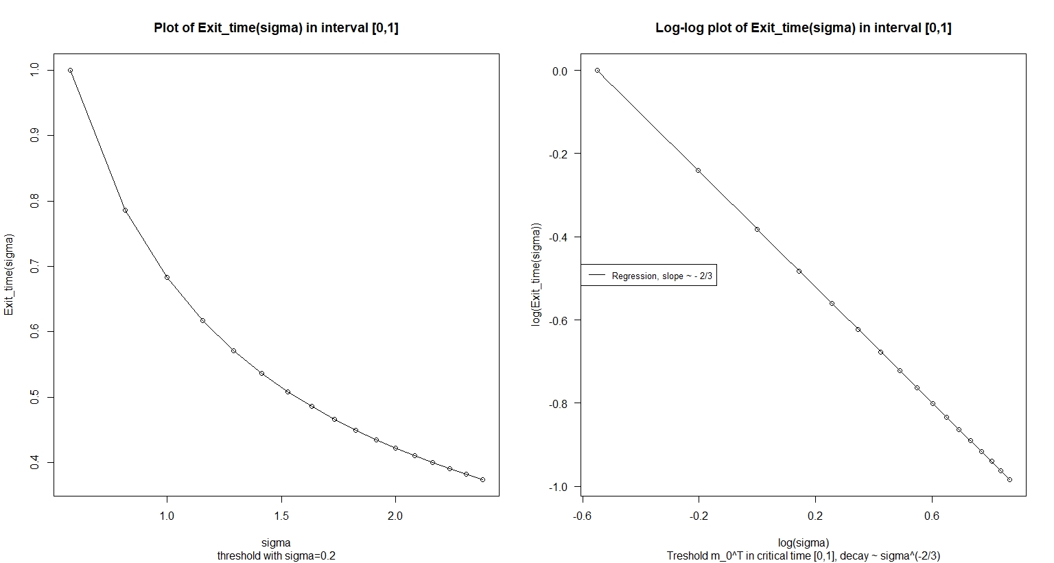
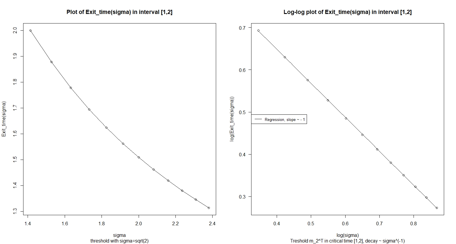
We see from Figures 3 and 4 that the expected behavior on the barrier time is obtained, and the curve exhibits a power like decay, with an asymptotic limit to zero. In Figure 3, we performed a log-log plot and regression taking and it yields (here and in the sequel denotes proportional to), whereas the same analysis in Figure 4 taking and considering only those exit times that are in the interval yields .
We conjecture that the function (18) can be expressed as (for suitably large, say in our simulations)
| (21) |
for some function that depends on dimension , and that . Here and in the sequel, denotes asymptotically for large .
A rough explanation of the numerical findings may be the following one, that will be explored more closely in a future work, since - as shown below - our understanding is still incomplete. When , the density of the unique level satisfies the identity
because the differential terms cancel by integration by parts. Assume that, at least after a transient time (confirmed by Figure 2), up to a small approximation,
namely the decay of is self-similar Eggers and Fontelos 2008. Then (up to approximation) where
is an average variation of velocity under , namely
after an initial transient period. Moreover, speculating that the standard deviation of should be of order (since the dispersion produced by the linear differential operator is proportional to ), we expect that increases linearly with . The numerical results of Figures 3 and 4 show that this looks the trend for sufficiently large time but for a short time another power, , emerges, that should be understood. As for the behavior in time, since this computation can be carried out for every , when , we believe that the decay in time is dimension-independent.


VII.2 Localized mass concentration:
When considering , we can expect two natural settings to investigate: the one where initially all the mass is concentrated on the first level, i.e. , and the one that follows the theoretical assumptions of Hammond and Rezakhanlou 2007; Flandoli et al. 2022b; Flandoli and Huang 2022. Concerning the first setting, we perform a numerical simulation of the system (16) for dimension , maximal mass level and time window .
In Figure 5, we plot the function (18) for different values of the turbulence parameter that ranges from , that we refer to as the non-turbulent case, to , which represents an intense eddy diffusivity. As in the case of , it shows a faster decay correlated to the increase of turbulence, and a speedup coagulation process.
For fixed , we perform a log-log plot in time window as shown in Figure 6 that shows is of inverse power approximately of , after a transient time period. Thus, we see a difference in the behavior of the “total mass” when increases: this is not unexpected when all the initial mass is concentrated in the first layer . In fact, analyzing the coagulation operator (5), we see that is responsable for the generation of bigger particles in higher mass-levels and it is dominant when all the mass of the system is selected as a single type. Therefore, for a transient period, we see an increase in mass for and as such a slower decay of , the total mass.
For this reason, as shown in Figure 7, we study the decay of the single mass , where analogous to (18), the single mass at level is defined as
| (22) |
The figure shows the regression curves plotted with dashed lines. As in Figure 2, for we maintain a relation of inverse power in time, approximately of , after a transient time period. As a further exploration, we see from Figure 8 that the same behavior is present, and the curve exhibits a power like decay, with an asymptotic limit to zero.

Concerning the behavior of the barrier time, we see from Figures 9 and 10 that the curve exhibits a power like decay, with an asymptotic limit to zero. In Figure 9, we perform a log-log plot and regression taking and it yields , whereas the same analysis in Figure 10 taking and considering only those exit times that are in the interval yields .


Thus, when , and the initial mass is located on a single level, we lose the conjectured behavior of Subsection VII.1, and we can only expect that the function (18) has the same asymptotic limit as
for some function that depends on dimension , and that . A rough explanation of this numerical finding may be the following one: when and the density is in the unique level , from (5) we see that the poisitive part is greater than the negative part for a transient period of time in which, for mass should increase before decay, suggesting a delay, and as such a reported slower decay, of the “total mass”. Also supporting this idea are the numerical simulations performed on the rapidity of decay for level . Here , and we see the same behavior as the limiting case in which only one type of mass is considered.

VII.3 Diffused mass concentration:
Here we propose a first analysis of the aformentioned second setting: the one that follows the theoretical assumptions as in Hammond and Rezakhanlou 2007; Flandoli et al. 2022b; Flandoli and Huang 2022. In detail, the initial mass is not concentrated only in one layer, but is generated according to two probability distributions so that with , and deterministic probability densities functions , , satisfying suitable regularity and decay assumptions, such that
| (23) |
As such, we select initial conditions compactly supported in a small range of velocity, i.e. , to better look at the behavior of the mass decay through time. We note here that this is the natural setting that generalizes the case of . We perform a numerical simulation of the system (16) for dimension , maximal mass level and time window .
In Figure 11, we plot the function (18) for different values of the turbulence parameter that ranges from , that we refer to as the non-turbulent case, to , which represents an intense eddy diffusivity. As in the case of , it shows a faster decay correlated with the increase of turbulence, and a speedup coagulation process. Plotted with dotted lines we show the decay of mass . This behavior is analogous for .
For fixed we perform a log-log plot in time window as presented in Figure 13. It shows that is of inverse power approximatly , after a transient time period dependent on the finiteness of the initial condition. As conjectured in the case , we see a consistency in the behavior of the “total mass” when increase: the initial condition is active everywhere, maintaining the structure of a probability density, thus making the results not unexpected. In fact, analyzing the coagulation operator (5), we see that is not dominant when all the masses of the system are spread over all the analyzed layers. Therefore, we see an immediate decrease in mass for and as such a maintained global decay of , the total mass.


For this reason, as shown in Figure 12, we study the decay of the single mass . The figure shows the regression curves plotted with dashed lines. As in Figure 2, we maintain a relation of inverse power in time, approximately of , after a transient time period. As a further exploration, we see that the same behavior is present, and the curve exhibits a power like decay, with an asymptotic limit to zero.
Concerning the behavior of the barrier exit time, we see from Figures 14 and 15 that the curve exhibits a power like decay, with an asymptotic limit to zero. In Figure 14, we perform a log-log plot and regression taking and it yields , whereas the same analysis in Figure 15 taking and considering only those exit times that are in the interval yields . Thus, when , and the initial mass is spread over all the mass levels, we are close to the conjectured behavior of previous section, and we can expect that the function (18) has the same asymptotic limit as
| (24) | |||
| (25) |

for some function that depends on dimension , and that . A rough explanation of this numerical finding may be the following one: when and the density is spread over all levels , from (5) we see that the positive part is already negligible with respect to that of , for all . In particular, the masses are drawn immediately to masses , that we interpret as falling rain outside of our system.
Supporting this we see in Figure 12 no transient period of time in which, for , mass increases before decaying, suggesting no delay, and as such the decay of the “total mass” is maintained. Note that and, as expected, we see the same behavior as the limiting case in which only one type of mass is condidered.
We summarize in Table 1 the precise fitting obtained through non-linear regression for all the analyzed quantities. The table shows accordance with our proposed decay behavior and suggests a future analysis for different initial conditions and higher dimensions.
| localized | diffused | ||
|---|---|---|---|
| -0.66 | -0.69 | -0.68 | |
| -0.94 | -0.92 | -0.91 | |
| -0.96 | -0.81 | -0.94 |
VII.4 Mean Collision Rate
Finally, in this segment we propose numerical simulations that validate the theoretical behavior proposed in Section VI.
In particular, we have analyzed the same setting as in 18, which either or . Computed with the procedure that we will explain below, all the case agree with equation 17 and the theory proposed in VI. As such, for visual clarity, here we illustrate results in the simpler case , with , and compute the behavior of and its law respect to the fluctuation parameter of the velocity, .
The same simulations, with , focusing on different mass level and different initial conditions are briefly discussed in Appendix C, Figure 19. There, computed limiting value show accordance with the simulations with .
From here on, we fix since objective of the paper is the understanding of the dependence on the turbulent kinetic energy of collision rate . However, we note that this parameter is important to the complete understanding of the behavior of this kind of systems, thanks to is relation with Stokes Number, and as such would be subject of future studies.
We know from 17 that a candidate estimation for is obtain throughout the steady state density of the system. For this reason, concerning the simulation, independently on , we selected a concentrated initial condition with moderate velocity and we let the system evolve in the time frame , producing solution .
Since no mass conservation is present for the finite system , and density is moved to higher levels not preserving the starting probability, we normalize at each time step the density , solution of our Smoluchowski equation, i.e. we consider
and, with this, the product probability . We are able to compute a time dependent, mean in velocity, collision rate:
In Figure 16, is shown the result for and this re-normalize collision rate. Each of the curves as an inverse behavior of a log-logistic function with exponent 1 in , suggesting a plateau in time. A such, this time dependent probability distribution on the product space of the velocity domains as a limiting density and we can argue that

In fact, as shown in Appendix C, Figure 20, the computed quantity approximate the theoretical limiting density , for this reason we initialize the evolving system with the proposed steady state condition , for different .
This means that we expect to be closer to the steady state distribution after a small time and the computed will be . As such, we restart the system with this new initial condition. To take into account that the velocity is spread, with value greater than one, and the total density near this high value is not negligible in comparison with the concentrated initial condition that we used throughout our experiment, we enlarged the velocity domain and the time domain to produce stable results on the decay of the masses and also on the mean rate .
In Figure 17 we show result on the re-started system, conferming the asymptotic limit of the collision rate and an increase in , the turbulent parameter of the system. We see a small flactuating period in which the rate is not increasing and than a fast stabilization that is linked to the velocity displacement of the steady state solution. In fact the new initial density condition produce, as expected, the same decay in the mass (since this depends only on and integral of the initial condition), but for a transient period the interaction kernel is much stronger that the speed in which diffusion of the Laplacian act, since the new initial condition is not negligible for high value of velocity. As such the plateau, which agrees with Figure 16, is reached after a small period of activation of the diffusion parameter.
Concluding, in Figure 18 we see that a linear relation with is present with angular coefficinet near , validating the expected behavior of with theoretical equation 17. This is expected and in line with the previuos reasoning and also with the small transient initialization.


VIII Conclusion
In this article, we presented a new kinetic model of a modified Smoluchowski PDE system with discrete and finite mass levels, that takes advantage of small scale turbulence and eddy diffusion in the velocity variable to enhance coagulation. We presented the derivation of the PDE system from a particle-fluid model subjected to a transport-type noise, and we analyzed numerically the behavior of its solutions. We showed that coagulation efficiency increases steadily with the increase of turbulence and, moreover, a power-law decay in time and in the turbulence parameter is present.Conluding, we have presented analytic and numerical presentation to understand the key factor of the collision rate as the average relative velocity between particles.
Appendix A Derivation of (4) from particle-fluid interaction
We present the sketch of the scaling limit to an SPDE from particle-fluid interaction for the truncated model (at threshold ).
For any and , consider an interacting particle system with space variable in , velocity variable in , mass variable in a finite set , and initial cardinality . Between coagulation events, the motion of an individual active particle obeys (recall (2))
| (26) |
where
- •
, is a given (at most countably infinite) collection of smooth, deterministic, divergence-free vector fields.
- •
is a given collection of standard Brownian motions in .
- •
denotes Stratonovich integration, according to Wong-Zakai principle Wong and Zakai 1965.
- •
is a positive constant that appears in Stokes’ law, that includes the dynamic viscosity coefficient of the fluid.
- •
is the set of indices of particles that are still active at time , with .
After each coagulation, the index set will change (decrease), and the velocity of a still-active particle will be reset according to the conservation of momentum, to be described a few paragraphs below.
We note again that the velocity component of the dynamics (A) obeys Stokes’ law for the frictional force exerted on a spherical particle immersed in a fluid, cf. Mehlig et al. 2007; Wilkinson et al. 2006, with the fluid velocity idealized by the white noise velocity field (12) (that acts simultaneously on all particles). This goes in the spririt of Kraichnan’s model Kraichnan 1968; Kazantsev 1968.
We denote the spatial covariance matrix of by
Moreover, for any fixed we denote the second-order divergence form elliptic operator, acting on suitable functions on
With suitable choice of , see Galeati 2020; Flandoli et al. 2021a; Flandoli et al. 2021b, we can have that
| (27) |
Each particle has a mass which changes over time according a stochastic coagulation rule to be described below. The initial mass , , are chosen i.i.d. (independent and identically distributed) from according to a probability distribution so that with . We are also given deterministic probability density functions , , satisfying suitable regularity and decay assumptions, such that if then the initial distribution of is chosen with probability density , independently across . We denote
| (28) |
The rule of coagulation between pairs of particles is as follows. Let be a given smooth symmetric probability density function in , that is, , with compact support in (the unit ball around the origin in ) and . Then, for any , denote by
Suppose the current configuration of the particle system is
where denotes the position, velocity and mass of particle , by convention if particle is no longer active in the system, we set (a cemetery state). Independently for each pair of particles, where run over the index set of active particles in , with a rate (derived from the collision kernel as in (Falkovich et al. 2002), compare with (9))
| (29) |
we remove from the configuration , and then in case , we add
with probability , and instead add
with probability . We call the new configuration obtained this way by and respectively. On the other hand, in case , then after removing from we do not add a new element.
In words, if coagulate, we decide randomly which of and is the new position of the mass-combined particle, provided that the combined mass does not exceed the threshold . If the position chosen is , then we consider as being eliminated (no longer active) and the new particle has index ; whereas if the position chosen is , then we consider as being eliminated and the new particle has index . On the other hand, the velocity of the mass-combined particle is obtained by the conservation of momentum as in perfectly inelastic collisions.
Note that the form of the coagulation rate (29) is such that a pair can coagulate only if , that is, their spatial positions have to be -close. We are interested in the case when as , so that the interaction is not of mean-field type, but local. Correspondingly, the final equation we get (see (32)) is local in the variable. In particular, choosing ensures that each particle typically interacts with a bounded number of others at any given time, which is the analogue in our continuum context, of nearest-neighbor or bounded-range interactions common in interacting particle systems defined on lattices, see Kipnis and Landim 1998 and references therein.
The essential feature of our coagulation rate is the presence of , which results in the same velocity difference appearing in the limit PDE (4). Although such rates are widely accepted in the physics literature on rain formations, our approach views as an active variable; we do not approximate it by a constant that depends on other physical parameters. Diffusion enhancement feeds back on coagulation enhancement through the presence of this velocity difference. As such, our Smoluchowski equation is new with respect to existing literature.
For each , and , we denote the process of empirical measure on position and velocity of mass- particles in the system by
| (30) |
where denotes the space of subprobability measures on equipped with weak topology. The choice of the initial conditions for our system implies that -a.s.
for , where indicates weak convergence of probability measures, and the limit (28) is absolutely continuous. We conjecture that, under the assumption of local interaction, i.e.
| (31) |
for every finite , the collection of empirical measures converges in probability, as , in , where is the space of càdlàg functions taking values in equipped with the Skorohod topology, towards an absolutely continuous limit . which is the pathwise unique weak solution to a Smoluchowski-type SPDE system (32). The latter SPDE degenerates to the PDE system we study in this paper (4) when the Itô term is switched off. Through recent progresses in stochastic fluid mechanics, cf. Galeati 2020; Flandoli et al. 2021a; Flandoli et al. 2021b; Flandoli et al. 2022c; Gess and Yaroslavtsev 2021, there exist specific limiting procedures that allow, in principle, to obtain the PDE from the SPDE by carefully choosing the vector fields . While we do not provide a rigorous proof here, we think that this heuristic argument is sufficient to justify our interest in studying our PDE system.
| (32) |
Appendix B Explanation of the link (3)
Recall the stochastic equation III. In real turbulent fluids, the fluid vector field is not exactly white in time, but has a correlation length approximately . Alleviating notations, let us only analyze the transport term involving and introduce a time delay of duration :
| (33) |
where the first equality is due to independent of , and in the last line we applied the equation III a second time (assuming the other terms are minor).
In the limit , approaches white noise in time, the first term of (B) yields a local-martingale, the Itô term. From the second term of (B) emerges a second-order elliptic operator
that in the limit is expected to converge to
Since the turbulence kinetic energy is the half-trace of the velocity covariance tensor Dupuy et al. 2019, idealizing the tensor structure of with , we may have that
and consequently,
This yields as claimed in (3).
In the above argument, it is crucial that we can take very small while having of order . With , the argument thus works only when is very large, and the regime where is of order requires a different analysis, consistent with the findings of Abrahamson 1975; Falkovich et al. 2002; Mehlig et al. 2007; Wilkinson et al. 2006.
Appendix C Mean Collision Rate and Guassianity assumption


Using the same method proposed in Section VII, we obtain analogous result for . We analyzed two initial condition: a localized one in the mass , and a theoretical one following Hammond and Rezakhanlou 2007. In both of this case we used the restarting limiting density either averaged or localized obtaining analogous results. In Figure 19, the case of localized density is shown with all combination of Collision Rate, showing agreement with the theory.
Finally, in Figure 20, we show the comparison between expected steady state probability and computed starting stationary solution , in the case and . The differecne in norm of the two functio is less then , as per the difference between thoeretical and computed estimated in less than , showing the same linear behavior.
References
- Abrahamson (1975) J. Abrahamson, Collision rates of small particles in a vigorously turbulent fluid, Chemical Engineering Science 30, 1371 (1975).
- Ayala et al. (2008) O. Ayala, B. Rosa, L.-P. Wang, and W. W. Grabowski, Effects of turbulence on the geometric collision rate of sedimenting droplets. part 1. results from direct numerical simulation, New Journal of Physics 10, 075015 (2008).
- Chun et al. (2005) J. Chun, D. L. Koch, S. L. Rani, A. Ahluwalia, and L. R. Collins, Clustering of aerosol particles in isotropic turbulence, Journal of Fluid Mechanics 536, 219 (2005).
- Devenish et al. (2012) B. Devenish, P. Bartello, J.-L. Brenguier, L. Collins, W. W. Grabowski, R. IJzermans, S. P. Malinowski, M. Reeks, J. Vassilicos, L.-P. Wang, et al., Droplet growth in warm turbulent clouds, Quarterly Journal of the Royal Meteorological Society 138, 1401 (2012).
- Falkovich et al. (2002) G. Falkovich, A. Fouxon, and M. Stepanov, Acceleration of rain initiation by cloud turbulence, Nature 419, 151 (2002).
- Falkovich and Pumir (2007) G. Falkovich and A. Pumir, Sling effect in collisions of water droplets in turbulent clouds, Journal of the Atmospheric Sciences 64, 4497 (2007).
- Grabowski and Wang (2013) W. W. Grabowski and L.-P. Wang, Growth of cloud droplets in a turbulent environment, Annual review of fluid mechanics 45, 293 (2013).
- Mehlig et al. (2007) B. Mehlig, V. Uski, and M. Wilkinson, Colliding particles in highly turbulent flows, Physics of Fluids 19, 098107 (2007).
- Papini (2021) A. Papini, Coagulation dynamics under random field: turbulence effects on rain, arXiv preprint arXiv:2111.12584 (2021).
- Pumir and Wilkinson (2016) A. Pumir and M. Wilkinson, Collisional aggregation due to turbulence, Annual Review of Condensed Matter Physics 7, 141 (2016).
- Reade and Collins (2000) W. C. Reade and L. R. Collins, A numerical study of the particle size distribution of an aerosol undergoing turbulent coagulation, Journal of Fluid Mechanics 415, 45 (2000).
- Saffman and Turner (1956) P. Saffman and J. Turner, On the collision of drops in turbulent clouds, Journal of Fluid Mechanics 1, 16 (1956).
- Shima et al. (2009) S.-i. Shima, K. Kusano, A. Kawano, T. Sugiyama, and S. Kawahara, The super-droplet method for the numerical simulation of clouds and precipitation: A particle-based and probabilistic microphysics model coupled with a non-hydrostatic model, Quarterly Journal of the Royal Meteorological Society: A journal of the atmospheric sciences, applied meteorology and physical oceanography 135, 1307 (2009).
- Sundaram and Collins (1996) S. Sundaram and L. R. Collins, Numerical considerations in simulating a turbulent suspension of finite-volume particles, Journal of Computational Physics 124, 337 (1996).
- Wang et al. (2005) L.-P. Wang, O. Ayala, S. E. Kasprzak, and W. W. Grabowski, Theoretical formulation of collision rate and collision efficiency of hydrodynamically interacting cloud droplets in turbulent atmosphere, Journal of the atmospheric sciences 62, 2433 (2005).
- Wilkinson et al. (2006) M. Wilkinson, B. Mehlig, and V. Bezuglyy, Caustic activation of rain showers, Physical review letters 97, 048501 (2006).
- Yeung and Pope (1988) P. Yeung and S. Pope, An algorithm for tracking fluid particles in numerical simulations of homogeneous turbulence, Journal of computational physics 79, 373 (1988).
- Flandoli et al. (2021a) F. Flandoli, L. Galeati, and D. Luo, Scaling limit of stochastic 2D Euler equations with transport noises to the deterministic Navier–Stokes equations, Journal of Evolution Equations 21, 567 (2021a).
- Flandoli et al. (2022a) F. Flandoli, L. Galeati, and D. Luo, Eddy heat exchange at the boundary under white noise turbulence, Philosophical Transactions of the Royal Society A 380, 20210096 (2022a).
- Galeati (2020) L. Galeati, On the convergence of stochastic transport equations to a deterministic parabolic one, Stochastics and Partial Differential Equations: Analysis and Computations 8, 833 (2020).
- Flandoli and Huang (2021) F. Flandoli and R. Huang, The KPP equation as a scaling limit of locally interacting Brownian particles, Journal of Differential Equations 303, 608 (2021).
- Flandoli and Huang (2022) F. Flandoli and R. Huang, Coagulation dynamics under environmental noise: scaling limit to SPDE, ALEA, Lat. Am. J. Probab. Math. Stat 19, 1241 (2022).
- Hammond and Rezakhanlou (2007) A. Hammond and F. Rezakhanlou, The kinetic limit of a system of coagulating Brownian particles, Archive for rational mechanics and analysis 185, 1 (2007).
- Flandoli et al. (2022b) F. Flandoli, R. Huang, and A. Papini, Smoluchowski coagulation equation with velocity dependence, arXiv preprint arXiv:2211.06693 (2022b).
- Kraichnan (1994) R. H. Kraichnan, Anomalous scaling of a randomly advected passive scalar, Physical review letters 72, 1016 (1994).
- Kraichnan (1967) R. H. Kraichnan, Inertial ranges in two-dimensional turbulence, The Physics of Fluids 10, 1417 (1967).
- Dupuy et al. (2019) D. Dupuy, A. Toutant, and F. Bataille, Effect of the reynolds number on turbulence kinetic energy exchanges in flows with highly variable fluid properties, Physics of Fluids 31, 015104 (2019).
- Eggers and Fontelos (2008) J. Eggers and M. A. Fontelos, The role of self-similarity in singularities of partial differential equations, Nonlinearity 22, R1 (2008).
- Wong and Zakai (1965) E. Wong and M. Zakai, On the convergence of ordinary integrals to stochastic integrals, The Annals of Mathematical Statistics 36, 1560 (1965).
- Kraichnan (1968) R. H. Kraichnan, Small-scale structure of a scalar field convected by turbulence, The Physics of Fluids 11, 945 (1968).
- Kazantsev (1968) A. Kazantsev, Enhancement of a magnetic field by a conducting fluid, Sov. Phys. JETP 26, 1031 (1968).
- Flandoli et al. (2021b) F. Flandoli, L. Galeati, and D. Luo, Delayed blow-up by transport noise, Communications in Partial Differential Equations 46, 1757 (2021b).
- Kipnis and Landim (1998) C. Kipnis and C. Landim, Scaling limits of interacting particle systems, Vol. 320 (Springer Science & Business Media, 1998).
- Flandoli et al. (2022c) F. Flandoli, L. Galeati, and D. Luo, Eddy heat exchange at the boundary under white noise turbulence, Philosophical Transactions of the Royal Society A 380, 20210096 (2022c).
- Gess and Yaroslavtsev (2021) B. Gess and I. Yaroslavtsev, Stabilization by transport noise and enhanced dissipation in the Kraichnan model, arXiv preprint arXiv:2104.03949 (2021).