Quantization and variational problem of the Gubser-Rocha Einstein-Maxwell-Dilaton model, conformal and non-conformal deformations, and its proper thermodynamics.

We must add to the gravitational action (2) a boundary action. This is to regularize its on-shell value as well as to make the variational principle well-defined. In the case of the scalar it also prescribes the quantization of the scalar field. We will be using in this work a standard multi-trace deformation of the Neumann boundary theory, which were generally described in Witten:2001ua; Mueck:2002gm; Papadimitriou:2007sj and more specifically in emd theories Caldarelli:2016nni, with a boundary action of the form

Here $N^{\mu}=-\sqrt{g^{zz}}(0,0,0,1)$ is an outward pointing spacelike unit normal vector defining the hypersurface $z=\epsilon\ll z_{h}$ and $\gamma_{\mu\nu}=g_{\mu\nu}-N_{\mu}N_{\nu}$ is the induced metric on the surface. Furthermore $K\equiv\gamma^{ij}K_{ij}$ is the trace of the extrinsic curvature $K_{ij}\equiv-\gamma_{i}^{\mu}\gamma_{j}^{\nu}\nabla_{(\mu}N_{\nu)}$ and ${}^{(3)}\!R_{\gamma}$ the Ricci scalar curvature of the hypersurface (Latin symbols correspond to coordinates on the hypersurface while the greek symbols are those of the original manifold). The first three terms correspond to the usual Gibbons-Hawking-York counterterms necessary to make the variational principle for the metric well-defined and also to regularize the Einstein-Hilbert-Cosmological Constant part of the action on shell. In our coordinatization Eq. (4) the induced metric is flat on-shell. The scalar part of the boundary term $S_{\mathrm{bdy},\phi}$ can take two forms depending on whether we consider the standard quantization boundary theory where only the $\phi^{2}$ regularization term appears

— here the value of $\Lambda_{\phi}$ is set to regularize the boundary term arising from varying the bulk action — or whether we consider a multi-trace deformation of the alternate quantization boundary theory

The $\phi N^{\mu}\partial_{\mu}\phi$ is a Legendre transform from Dirichlet to Neumann boundary conditions, which also diverges at leading order and is the reason for the shift in $\Lambda_{\phi}$ as we will see.⁴⁴ 4 Strictly speaking $\phi N^{\mu}\partial_{\mu}\phi$ is a combination of a true Legendre transform $J{\cal O}=z^{\lambda_{-}-\lambda_{+}-1}\phi\partial_{n}z^{-\lambda_{-}}\phi$ (see Eq. (13)) and counterterms. The multi-trace deformation $S_{F}$ is a finite contribution to the boundary action and will be described when the asymptotics of the solution are analysed. We will continue the derivation with the choice $S_{\mathrm{bdy},\phi}=S_{\mathrm{bdy},\phi}^{(\mathrm{MT})}$ while keeping in mind that a similar derivation can easily be done using instead $S_{\mathrm{bdy},\phi}=S_{\mathrm{bdy},\phi}^{(\mathrm{SQ})}$, and we will invoke those results when necessary.

Varying the total action $S=S_{\mathrm{bulk}}+S_{\mathrm{bdy}}$ to first order, a proper holographic interpretation demands that one obtains a variation of the form Balasubramanian:1999re

where the terms multiplying the emd fields are interpreted as the operators in the boundary CFT where $T_{\mu\nu}$ is the boundary stress tensor, $J_{\mu}$ the boundary current associated with the U(1) charge, and $\mathcal{O}_{\varphi}$ the operator dual to a scalar which may be a non-linear function of the dilaton field. The important point is that the action evaluated on the black hole solution is equated with (minus) its Gibbs free energy density. The variation of the action (restricted to preserve isotropy) thus includes thermodynamic variations. The expression above makes clear that in addition to the temperature and the chemical potential there ought to be a dependence of the Gibbs free energy on an external (source) variation of (the boundary value of) the scalar field Li:2020spf.

Performing this variation on Eqs (2) plus (7), we can write it as a bulk integral of an integrand proportional to the equations of motion (3), that vanishes on-shell, and a remaining boundary part. In the boundary part the normal derivatives of $\delta\gamma_{\mu\nu}$ cancel due to the Gibbons-Hawking-York term; there are no normal derivatives in $A_{\mu}$. Restricting to boundary indices we have⁵⁵ 5 The radial components of $T_{\mu\nu}$ and $J_{\mu}$ vanish due to the projection on the hypersurface.

where $T_{ij}^{F}$ is the contribution from $S_{F}$. The expression for $\mathcal{O}_{\varphi}$ requires a more detailed discussion. Focusing on the variation in the dilaton $\phi$ in (10), we have

From its linearized equation of motion the dilaton has the following expansion in the near-boundary region

where $\lambda_{\pm}=\dfrac{3}{2}\pm\dfrac{1}{2}\sqrt{9+4m^{2}}$ and $m$ is the effective mass. In the gr model the effective mass equals

This value of the mass $-\frac{9}{4}<m^{2}<1-\frac{9}{4}=-\frac{5}{4}$ is in the regime where two different quantizations are allowed, i.e. for this value of $m$ both $\lambda_{\pm}>0$ and either $\alpha$ (standard) or $\beta$ (alternate) can be chosen as the source for the dual CFT operator with the other the response. One can also choose a mixture of the two, corresponding to a multi trace deformation, as we shall elucidate below.

The proper holographic normalization is most conveniently performed in a fg ansatz for the metric

where we require Anti-deSitter (AdS) aymptotics $H_{\mu\nu}(z=0)=1$ and use the equations of motion (3) to constrain the near-boundary expansion of $H_{\mu\nu}$ in terms of a small subset of degrees of freedom. We will use this ansatz for the remainder of this section. Using that $N^{z}(z)=-z$, and substituting (13) into (12), we can expand the variation w.r.t. the dilaton as

As we claimed in (9), we must remove the leading divergence by imposing $\Lambda_{\phi}=1$, leaving a finite contribution

For the standard quantization term (8), it is easy to see that a similar derivation leads to $\Lambda_{\phi}=-1$.

One can modify the quantization by the addition of a multitrace deformation. This can in general be encoded in the boundary action $S_{F}$. Following Papadimitriou:2007sj; Vecchi:2010dd; Caldarelli:2016nni, we choose $S_{F}=\int\differential^{3}x\sqrt{-\gamma}\epsilon^{d}\mathcal{F}(\alpha)$ such that, ignoring the metric variation, $\delta S_{F}=\int\differential^{3}x\sqrt{-\gamma}\epsilon^{d}\mathcal{F}^{\prime}(\alpha)\delta\alpha$. Without loss of generality we choose $\mathcal{F}$ of the form $\mathcal{F}(\alpha)=\frac{a}{2}\alpha^{2}+\frac{b}{3}\alpha^{3}$ from here on. The variation of the boundary action then becomes

We can therefore identify the VEV of the boundary scalar operator as $\mathcal{O}_{\varphi}=\alpha$ while the source of the operator is

Once again, had we chosen the standard quantization boundary term, then we would have $\delta S_{\phi}=\int\differential^{3}x\beta\delta\alpha$ such that $\mathcal{O}_{\varphi}=\beta$ and $\varphi=\alpha$ leading to the boundary condition $J_{\mathrm{SQ}}=\alpha$.

We have now almost all the ingredients to compute the scalar contribution to the stress tensor, but we still need to derive the variation of $S_{F}$ w.r.t. the leading order of the boundary metric in order to compute the term $T_{ij}^{F}$, as was done before in Caldarelli:2016nni. Doing so, one simply finds $T^{F}_{ij}=\gamma_{ij}\epsilon^{d}\mathcal{F}(\alpha)$. It is interesting to note that the contribution $S_{F}$ can also be absorbed into corrections to the $\phi^{2}$ term as well as a $\phi^{3}$ term as

where $\Lambda_{\phi}+\epsilon a$ is a renormalized $\phi^{2}$ coupling which will reproduce the $\alpha^{2}$ contribution of $\mathcal{F}$, as was done in e.g. Witten:2001ua; Bernamonti:2009dp. The $\phi^{3}$ coupling on the other end will reproduce the $\alpha^{3}$ contribution of $\mathcal{F}$. This way of writing the boundary action action highlights why we concentrated on $\mathcal{F}$ of the form $\mathcal{F}(\alpha)=\frac{a}{2}\alpha^{2}+\frac{b}{3}\alpha^{3}$. Lower order in $\alpha$ terms are constant shifts variationally and can be absorbed in a field redefinition – they are tadpoles. Any term $\alpha^{n}$ for $n>d$ would lead to vanishing contributions $\epsilon^{n-d}$ in the action – they are irrelevant deformations. The equality $\Lambda_{\phi}=1$ remains true in order to regularize $\delta S$.

In the presence of such a boundary action, the contribution $T_{ij}^{F}$ in the expression (11) simply includes the $\phi^{2},\phi^{3}$ contributions and leads to

We recognize the $\mathcal{F}$-dependent part of the stress tensor which agrees with the direct method. It is then immediate to compute the trace of the stress tensor

where in the last equality we used the boundary condition (19). This result points to the existence of a line of critical points with $a=0$ where the sourceless ($J_{\mathrm{MT}}=0$ equivalent to the boundary condition $-\beta+a\alpha+\frac{b}{2}\alpha^{2}=0$) deformation $\mathcal{F}$ is just marginal. This is equivalent to only deforming the boundary theory through a $\phi^{3}$ term which indeed has dimension $d$ and should therefore be marginal.

For completeness we mention that in the case of the standard quantization the trace of the stress tensor is simply $T_{i}{}^{i}=\alpha\beta=\beta J_{\mathrm{SQ}}$.

In this subsection, we will derive the thermodynamics of a black hole solution in a general compatible quantization choice. This goes beyond the analyses in Kim:2016dik; Caldarelli:2016nni where only the thermodynamics of a marginal scalar were considered, i.e. the case of alternate quantization with a multitrace deformation such that the stress tensor remains traceless. In view of extending the choice of possible theories to non-marginal ones, we will show that the thermodynamics space is extended from a 2-parameter to a 3-parameter space, as also emphasized for Einstein-Scalar theory in Li:2020spf.

Let us start with the constraint that a choice of solution imposes on the possible quantization schemes. Indeed, while the choice of boundary terms in the action and therefore of the boundary deformation is a priori agnostic of a given solution to the bulk equations of motion, we have seen that the multi-trace deformation leads to a specific choice of boundary condition on the scalar (19). Not every solution to the bulk equations of motion (3) are compatible with every possible boundary condition, as was noted in Caldarelli:2016nni; Ren:2019lgw. In the case of the metric corresponding to the agr solution (5), the scalar $\phi$ has the following falloffs

where we have related the values of $\phi^{\prime}(0),\phi^{\prime\prime}(0)$ to the falloffs $\alpha,\beta$ in the fg ansatz (15). This matching is made explicit in Section B. Comparing with the full solution (5), we can therefore equate $\alpha=\sqrt{3}Q/2$ and $\beta=\sqrt{3}Q^{2}/8$. Consider then alternate quantization deformed by an arbitrary (relevant and marginal) multitrace deformation. In that case the source equals

From this equation, we see there are a few distinct cases to consider

1. 1.

   $a=0,b=b_{\mathrm{aGR}}\equiv 1/\sqrt{3}$: every instance of the 2-parameter agr solution (5) is compatible with this choice and is sourceless $J=0$. This is the sourceless marginal deformation we previously mentioned and which was studied in Kim:2016dik; Caldarelli:2016nni; Ren:2019lgw. From Eq. (22), we see that this boundary theory has $T_{i}{}^{i}=0$.

2. 2.

   $a=0,b=0$: the quantization procedure is conventional alternate quantization. In this case, since the solution (5) is not sourceless, we must impose a Neumann boundary condition $\beta=-J$ with fine-tuned source $J(Q)=-\sqrt{3}Q^{2}/8$. The explicit source leads to an explicitly broken conformal symmetry in the boundary. (A similar argument holds for standard quantization with a Dirichlet boundary condition $\alpha=J$. One would then need to consider the boundary term $S_{\mathrm{bdy},\phi}=S_{\mathrm{bdy},\phi}^{(\mathrm{SQ})}$ instead, and a fine-tuned source $J(Q)=\sqrt{3}Q/2$. Also here the explicit source leads to an explicitly broken conformal symmetry in the boundary.)

3. 3.

   For all the other cases, one can look for explicitly sourced solutions $J=J(Q,a,b)$ defined in Eq. (24).⁶⁶ 6 If we insist on looking for solutions with $J=0$, one of the couplings $a$ or $b$ must be fine-tuned e.g., $b(Q)=\frac{1}{\sqrt{3}}(1-4a/Q)$. As it was noted in Ren:2019lgw, this means that fixing $a,b$ to some constant will restrict the space of solutions to those for which $Q=\frac{4a}{1-\sqrt{3}b}$. Allowing for a finite, albeit fine-tuned, source $J=J(Q)$ leads to the same result and we will choose this more natural point of view. This case is fundamentally similar to the case 2, with the explicit sourcing leading to a non-zero trace of the boundary stress-tensor.

In the end, we see that the only natural sourceless description we have of the solutions (5) corresponds to the marginal multi-trace deformation, case 1. The other cases, 2 and 3, are better understood as explicitly sourced deformations where the source is fine-tuned to select a certain subset of solutions at a fixed $Q$.

An important aspect is that even though a bulk solution may have different interpretations depending on the quantization choices set out above, the thermodynamics does know about the quantization choice. Let us consider the free energy of the solutions (5). Substituting the solution into the action, the free energy density $\Omega$ of the agr black hole solution with compatible boundary condition is given by

Furthermore, the holographic dictionary tells us that the chemical potential and the temperature of the boundary theory are given by (6). One might be inclined to use this to deduce a variation of $\Omega$ in the 2-parameter grand canonical ensemble $\differential\Omega=-s_{1}\differential T-\rho_{1}\differential\mu$ and derive from it the thermodynamic entropy and charge density of the theory

However, we have seen from Eq. (10) that the free energy variation in the presence of an explicit source should be corrected by a scalar contribution of the form (see also Li:2020spf)

This is the full 3-parameter thermodynamics of the system. The fact that the free energy (25) of the agr solution only depends on $T$ and $\mu$, and not on the value of the scalar source means that the agr solution should be seen as a 2-parameter constrained solution within this 3-parameter space. This family of solutions is only a subset of all the possible ones for any given compatible quantization scheme. A direct corollary is that to explore only this analytical set of solutions, variations of $J,T,\mu$ are not independent. Denoting $J$ as the dependent variable, i.e. it is not independent but is a function of both $T$ and $\mu$, then the grand canonical potential varies as

if one constrains one’s considerations to agr solutions only.

The precise relation of the VEV $\mathcal{O}_{\varphi}$ and the source $J$ to the fall-off of the dilaton depends on the quantization scheme as we have just reviewed. A choice of quantization is not a canonical transformation, as shown by Li:2020spf in the standard quantization case for Einstein-Scalar theories. Therefore the value of the free energy will depend on this choice. This is evident in the dependence on $a,b$ in Eq. (25). In the full 3-parameter space of solutions this quantization choice dependence would only appear in the dilaton contribution part. In the constrained 2-parameter space of solutions, it would appear to imply that now also the thermodynamic entropy $s_{1}$ and charge density $\rho_{1}$ deduced from Eq. (26) depend on the quantization, as

This is strange, as the Bekenstein-Hawking entropy and the charge density – the VEV of the sourced gauged field – are properties of the black hole solution and do not depend on the boundary action which sets the quantization. Indeed they can be read off directly from the geometry as

The solution is of course that in the constrained system $s_{1}$ and $\rho_{1}$ are not the true entropy and charge density, as they include the artificial contribution from varying $J(T,\mu)$ following from the constraint to stay within the 2-parameter agr solution space. It is then a rather straightforward computation to connect Eqs. (29) and (30) through the variation of $J$ expressed in Eq. (27). To that end, we can remember that the source $J$ is constrained by the boundary condition (24) and that in our choice of quantization, we always have $\mathcal{O}_{\varphi}=\alpha$. In summary, the geometric expressions for the entropy and charge of the agr solution are always the correct ones. The difference from the quantities computed from the Gibbs potential can be attributed to the fact that one considers a constrained system: the expression $s_{1}=-\left(\frac{\partial\Omega}{\partial T}\right)_{\mu}=-\left(\frac{\partial\Omega}{\partial T}\right)_{\mu}-\mathcal{O}_{\varphi}\left(\frac{\partial J}{\partial T}\right)_{\mu}$ contains a term that is absent in the correct definition of the entropy $s_{2}=-\left(\frac{\partial\Omega}{\partial T}\right)_{\mu,J}$, and similarly for $\rho$.

There is, however, the special case 1. When the deformation is purely marginal and sourceless – $a=0$ and $b=\frac{1}{\sqrt{3}}$ – we can immediately infer that the variations of $J=0$ will be trivial. In that case, we will have $s_{1}=s_{2}$ and $\rho_{1}=\rho_{2}$. The way to understand this is that within the 3-parameter space of possible solutions quantified by $(T,\mu,J)$ the 2-parameter agr solution spans a different subspace depending on the quantization choice for the dual boundary theory. Figure 1, illustrates how this difference of boundary interpretation between the alternate quantization with sourceless marginal deformation of case 1 and the standard quantization of case 2 changes the shape of the agr solution manifold inside the thermodynamic space of sources $\{T,\mu,J\}$. This visualization allows us to see at a glance how the sourceless marginal deformation reduces to a 2-charge thermodynamic space where 2-parameters of the solution naturally coincide with $T,\mu$ while the standard quantization interpretation of the agr solution induces some non-trivial projection when varying the Gibbs free energy w.r.t. $T,\mu$. For the sourceless marginal deformation the thermodynamics of the boundary thus simplifies greatly and will behave in a similar fashion to the conformal fluid dual to the rn black hole solution.

To complete the argument above we shall construct numerical solutions to the equations of motion (3) in the next section that differ from the agr solution in that they explore the third direction orthogonal to $T,\mu$ and analyse their various boundary interpretations.

The solutions that generically differ from (5) correspond to setting different boundary conditions for the dilaton field. However, for each such new solution, its interpretation depends on the quantization one considers, i.e. what the on-shell value of the action including boundary terms reads.

We will solve the gr equations of motion (3) numerically using the following parametrization

and with metric ansatz

where $f(z),g(z),j(z)$ are held fixed to their expressions in the agr solution (5) and $\psi,a_{t},G_{tt},G_{zz},G$ are the dynamical fields. The radial coordinate $z$ spans the range from the boundary at $z=0$ to the outer horizon at $z=z_{h}$. The IR boundary conditions are chosen to have a single zero horizon corresponding to a non-extremal black hole and to impose regularity at the horizon for other fields (see e.g., Horowitz:2012ky).⁷⁷ 7 The boundary conditions from regularity imply in particular that $G_{tt}(z_{h})=G_{zz}(z_{h})$. This conveniently allows us to set the temperature with the parameters $Q$ and $z_{h}$ just like in the agr solution in Eq. (6), as the temperature of this generalised model is given by $T=T_{\mathrm{GR}}\sqrt{G_{tt}(z_{h})/G_{zz}(z_{h})}=3\sqrt{1+Qz_{h}}/{4\pi z_{h}}$. The UV boundary conditions are chosen to impose AdS asymptotics for the metric components and $A_{t}(0)=\mu$. Parametrizing $\mu=\sqrt{3Qz_{h}(1+Qz_{h})}/z_{h}$ as in the agr solution, the scalar boundary condition (19) can be rewritten in terms of the falloffs of $\psi$ as

For simplicity, we will choose $z_{h}=1$ and the temperature of the solutions will therefore be encoded by $Q=\frac{3\mu^{2}}{16\pi^{2}T^{2}}$. In holography, we would usually first fix the boundary theory of interest by choosing $a,b$. Then every solution to the equations of motion would be labeled by $(T,\mu,J)$ imposed through the boundary conditions. However in this section, we will be interested in how a given set of solutions, labeled by $(T,\mu,\psi(0))$, behaves in the various compatible boundary theories. This is possible because the boundary condition we impose on the scalar is simply a way to parametrize how we choose a bulk solution constrained to have a black hole in the interior. Every boundary theory determined by $a,b$ and the value of sourcing $J$ compatible with the condition (33) will provide a valid boundary description. We will focus on the boundary interpretations in the next subsection. In many holographic studies $\psi(0)$ is often used interchangeably with the source $J$, but this is of course only true in standard quantization. We shall, however, be careful to distinguish between the boundary value $\psi(0)$ of the AdS scalar field and the source $J$ of the operator in the quantization choice dependent dual field theory.

Let us now briefly describe the effect of changing $\psi(0)$ without referring to any specific boundary theory. By looking at the agr solution (5), we see that $\psi(0)=Q\sim(T/\mu)^{-2}$ for this family. Therefore, increasing $\psi(0)$ is akin to lowering the temperature and vice versa. To confirm our intuition, we can compare solutions at fixed $Q_{0}\sim(T_{0}/\mu)^{-2}$, and varying $\psi(0)$, to agr solutions with $\psi(0)=Q\neq Q_{0}$ i.e., at different $T/\mu\neq T_{0}/\mu$. We will choose to focus on the gauge field $A_{t}(z)$ and more specifically the component $a_{t}(z)$ defined in (31). Formally, $a_{t}(z)=A_{t}(z)/(\mu j(z,T_{0}/\mu))$ for a fixed $T_{0}/\mu$. Since the agr solution at a different temperature $T/\mu$ will have a gauge field $A_{t}(z)=\mu j(z,T/\mu)$, the correct field to compare with will be $a^{\psi(0)=Q}_{t}(z,T/\mu\neq T_{0}/\mu)=j(z,T/\mu)/j(z,T_{0}/\mu)$. We plot the profiles $a_{t}^{\psi(0)\neq Q_{0}}(z,T_{0}/\mu)$ in Figure 2 and compare these to $a_{t}^{\psi(0)=Q}(z,T/\mu>T_{0}/\mu)$ (purple) and $a_{t}^{\psi(0)=Q}(z,T/\mu<T_{0}/\mu)$ (red). We see that indeed, starting from $\psi(0)=Q_{0}$, as we increase (decrease) $\psi(0)$ with $Q_{0}$ fixed, the solution becomes similar to the agr solution at lower (higher) $T/\mu$.

Having numerically constructed instances of this one-parameter deformation of fixed $T/\mu$ gr black holes, each instance in turn has multiple holographic dual interpretations depending on the quantization scheme. These are constrained by the compatibility condition (33). We will focus on three specific choices:

1. 1.

   the conformal symmetry preserving quantization $a,J=0$ boundary theory for which we can then label our solutions by $b(\psi(0))=\frac{4}{\sqrt{3}\psi(0)^{2}}\left(\psi^{\prime}(0)+\frac{3Q}{4}\psi(0)\right)$,

2. 2.

   the standard quantization boundary theory with the label $J=\alpha=\frac{3}{2}\psi(0)$,

3. 3.

   the alternate quantization boundary theory with $a,b=0$ for which the label is now $J=-\beta=-\frac{3}{2}\psi^{\prime}(0)-\frac{3\sqrt{3}Q}{8}\psi(0)$.

Using Eq. (11) we can compute the energy and the pressure of a solution in a specific quantization scheme and construct the trace of the stress tensor $T_{i}{}^{i}=-\epsilon+2P$ for each of these solutions. For the choice 1, as we can see in Figure 3, the stress tensor remains traceless for any value of $b(\psi(0))$, confirming the analytic result Eq. (22). This is what we expect from a CFT deformed by a marginal operator. On the other hand, for the choice 2, we see that generically conformality is broken and the stress tensor acquires a non zero trace. In this quantization scheme, this is also true for the agr solution, as we described in the case 2. There are two exceptions: the first one is when $J=0$ (but $\mathcal{O}_{\varphi}\neq 0$) – which is reminiscent of a $\mathbb{Z}_{2}$ spontaneously symmetry breaking solution but here, the finite charge of the black hole actually always leads to an explicitly symmetry broken (ESB) solution $\phi(z)\neq 0$. This case is outside the range of the plot Figure 3. The second solution would happen around $J/Q\approx 1.4$ such that $\mathcal{O}_{\varphi}=0$. These are consistent with what we would have expected from $T_{i}{}^{i}=\alpha\beta$.

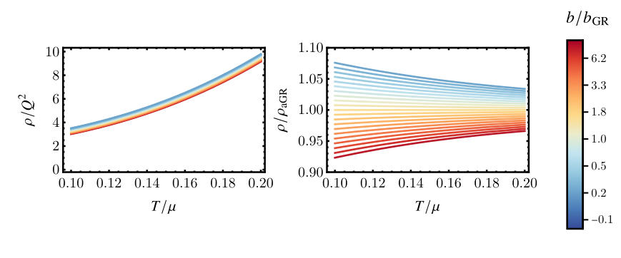
Each one of these new black hole solutions has a different thermodynamics compared to the agr solution. A clean way to exhibit this is to show the boundary charge density $\rho_{2}$, which for the choice 1 is the same as the variation of the Gibbs free energy w.r.t. the chemical potential, i.e. in that case $\rho_{2}=\rho_{1}$. In Figure 4, we plot the charge density as a function of temperature for various values of the marginal coupling $b$. It is clear from this figure that the charge density as a function of $T/\mu$ is dependent on the choice of boundary theory and the deformed solution describes a different state, even if the change is small.

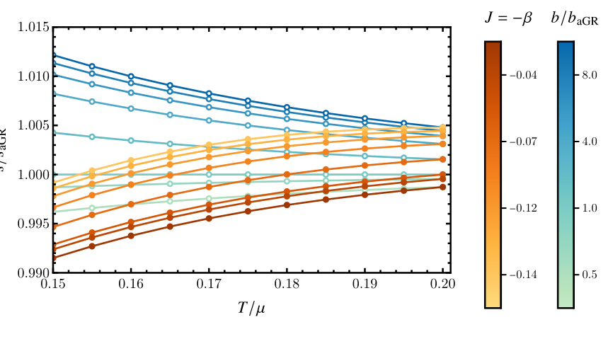
To reiterate this last point, let us remember that a priori, the true charge density of the theory $\rho_{2}$, as well as the true entropy of the theory $s_{2}$, only depend on the bulk solution – they are geometric quantities. Yet we now argue that different boundary theories have different thermodynamics. The resolution of this apparent contradiction is that while the entropy and charge density of a black hole solution only really depend on the bulk solution, how we explore the space of solutions is dependent on the choice of quantization. As we mentioned in Section 4, the holographic interpretation of black hole thermodynamics shows that we should label solutions by their sources $\{T,\mu,J\}$ – and in the case of the sourceless solutions of the choice 1, $b$ plays the role of the label $J$. But different boundary theories have different notion of source $J$ such that varying $T$ and $\mu$ at fixed $J$ will mean different path in the space of bulk solutions labeled by $\{T,\mu,\psi(0)\}$. In Figure 5, we illustrate this point by looking at the Bekenstein-Hawking entropy $s_{2}$ as a function of $T/\mu$ – all solutions are normalized by the agr entropy defined in (30). Both choices 1 and 3 are used to label the solutions when varying the temperature, which can be done by imposing the boundary condition (33) for each of the choices. The values of $b(\psi(0))$ and $J=-\beta$ are chosen such that solutions meet in pair at $T/\mu=0.2$. Upon lowering the temperature, we see that these pairs split indicating that the bulk solutions they belong to are not the same anymore. A path at fixed $J=-\beta$ is therefore generically different than a path at fixed $J=\alpha$ or fixed $b(\psi(0))$.

References

- [1] Thomas Faulkner, Hong Liu, John McGreevy, and David Vegh. Emergent quantum criticality, Fermi surfaces, and AdS(2). Phys. Rev. D, 83:125002, 2011.
- [2] Christos Charmousis, Blaise Gouteraux, Bom Soo Kim, Elias Kiritsis, and Rene Meyer. Effective Holographic Theories for low-temperature condensed matter systems. JHEP, 11:151, 2010.
- [3] B. Gouteraux and E. Kiritsis. Generalized Holographic Quantum Criticality at Finite Density. JHEP, 12:036, 2011.
- [4] Liza Huijse, Subir Sachdev, and Brian Swingle. Hidden Fermi surfaces in compressible states of gauge-gravity duality. Phys. Rev. B, 85:035121, 2012.
- [5] Qimiao Si, Silvio Rabello, Kevin Ingersent, and J. Lleweilun Smith. Locally critical quantum phase transitions in strongly correlated metals. Nature, 413(6858):804–808, October 2001.
- [6] Steven S. Gubser and Fabio D. Rocha. Peculiar properties of a charged dilatonic black hole in . Phys. Rev. D, 81:046001, 2010.
- [7] Kevin Goldstein, Shamit Kachru, Shiroman Prakash, and Sandip P. Trivedi. Holography of Charged Dilaton Black Holes. JHEP, 08:078, 2010.
- [8] Yi Ling, Chao Niu, Jian-Pin Wu, and Zhuo-Yu Xian. Holographic Lattice in Einstein-Maxwell-Dilaton Gravity. JHEP, 11:006, 2013.
- [9] Richard A. Davison, Koenraad Schalm, and Jan Zaanen. Holographic duality and the resistivity of strange metals. Phys. Rev. B, 89(24):245116, 2014.
- [10] Bom Soo Kim. Holographic Renormalization of Einstein-Maxwell-Dilaton Theories. JHEP, 11:044, 2016.
- [11] Marco M. Caldarelli, Ariana Christodoulou, Ioannis Papadimitriou, and Kostas Skenderis. Phases of planar AdS black holes with axionic charge. JHEP, 04:001, 2017.
- [12] Edward Witten. Multitrace operators, boundary conditions, and AdS / CFT correspondence. 12 2001.
- [13] Wolfgang Mueck. An Improved correspondence formula for AdS / CFT with multitrace operators. Phys. Lett. B, 531:301–304, 2002.
- [14] Li Li. On Thermodynamics of AdS Black Holes with Scalar Hair. Phys. Lett. B, 815:136123, 2021.
- [15] Ioannis Papadimitriou. Multi-Trace Deformations in AdS/CFT: Exploring the Vacuum Structure of the Deformed CFT. JHEP, 05:075, 2007.
- [16] Vijay Balasubramanian and Per Kraus. A Stress tensor for Anti-de Sitter gravity. Commun. Math. Phys., 208:413–428, 1999.
- [17] Luca Vecchi. Multitrace deformations, Gamow states, and Stability of AdS/CFT. JHEP, 04:056, 2011.
- [18] Alice Bernamonti and Ben Craps. D-Brane Potentials from Multi-Trace Deformations in AdS/CFT. JHEP, 08:112, 2009.
- [19] Jie Ren. Analytic solutions of neutral hyperbolic black holes with scalar hair. Phys. Rev. D, 106(8):086023, 2022.
- [20] Gary T. Horowitz, Jorge E. Santos, and David Tong. Optical Conductivity with Holographic Lattices. JHEP, 07:168, 2012.
- [21] Ethan Dyer and Kurt Hinterbichler. Boundary Terms, Variational Principles and Higher Derivative Modified Gravity. Phys. Rev. D, 79:024028, 2009.