A two-component vector WIMP – fermion FIMP dark matter model with an extended seesaw mechanismPreprint: CERN-TH-2022-155
Abstract
We consider an extension of the Standard Model that explains the neutrino masses and has a rich dark matter phenomenology. The model has two dark matter candidates, a vector WIMP and a fermion FIMP, and the sum of their relic densities matches the total dark matter abundance. We extensively study the dark matter production mechanisms and its connection with the neutrino sector, together with various bounds from present and future experiments. The extra scalar field in the model may induce a first-order phase transition in the early Universe. We study the production of stochastic gravitational waves associated with the first-order phase transition. We show that the phase transition can be strong, and thus the model may satisfy one of the necessary conditions for a successful electroweak baryogenesis. Detectability of the phase transition-associated gravitational waves is also discussed.
1 Introduction
The Standard Model (SM) of particle physics has proved extremely successful in the past decades with the experiments matching its predictions and the Higgs boson discovery being the final piece to complete it. Nonetheless, astrophysical and cosmological evidence have posed questions that are not explained by the SM and are still open problems to this date.
It is well established by neutrino oscillation data (NOD) that the neutrinos have a non-zero mass while in the SM they are massless. A mechanism is therefore needed to generate the masses Super-Kamiokande:1998kpq; Gonzalez-Garcia:2002bkq. The neutrinos are not only massive, but their masses are also much lighter than the other matter particles. The mass splitting between the first and the second eigenstates is , and the mass gap between the second and the third is Esteban:2020cvm. Also, from cosmological data, the sum of the neutrino masses is bounded by Planck:2015fie; Planck:2018vyg. These observations are calling for a new mechanism. Arguably the easiest and first proposed mechanism is the so-called type-I seesaw Minkowski:1977sc; Gell-Mann:1979vob, where heavy singlet leptons are introduced: The mixing between the heavy singlet leptons and the light neutrinos can generate a small mass since the light neutrino masses are suppressed by the heavy mass scale, resulting in where is of the order of the heavy lepton mass, is the SM Higgs vacuum expectation value (VEV), and is the light neutrino Yukawa coupling.
An extended version of the type-I seesaw mechanism, dubbed extended double seesaw Kang:2006sn; Mitra:2011qr, where a second set of singlet neutrinos is added, was proposed to achieve a low-scale leptogenesis without a fine tuning of the heavy neutrino masses; see also Ref. Majee:2008mn for an ultraviolet (UV) completion. The attractiveness of the low-scale leptogenesis is its detection possibilities from future collider experiments. In addition, the supersymmetric version of the extended double seesaw mechanism avoids the gravitino problem Kang:2006sn; Kawasaki:2004qu; see also Ref. Hook:2018sai. Notably, the double seesaw mechanism allows us to consider Yukawa couplings for the extra neutrinos up to with masses at the TeV scale, having the possibility to be probed by future collider experiments.
The dark matter (DM) is another missing piece of the SM. We have cosmological evidences that indicate that our Universe is composed of 23% of DM. These observations point towards cold, dark, and particle-like explanations Ostriker:1973uit; Planck:2018vyg; Corbelli:1999af. The standard solution to the problem is a Weekly Interacting Massive Particle (WIMP) which is initially in thermal contact with the SM thermal bath in the early Universe. At some later time, it freezes out, producing the relic density observed today that is inversely proportional to the thermal cross section Gunn:1978gr; Hut:1977zn; Lee:1977ua; Bertone:2004pz.
Alternative mechanisms have been explored with increasing interest since the effort to detect a WIMP-like particle has been unsuccessful up to now XENON:2018voc; CMS:2016lcl; MAGIC:2016xys; Arcadi:2017kky; PandaX-II:2016vec; LUX:2016ggv. In particular, the freeze-in mechanism has gained tremendous attention in the past two decades McDonald:2001vt; Choi:2005vq; Kusenko:2006rh; Hall:2009bx; Cheung:2011nn; Elahi:2014fsa; Arcadi:2015ffa; Bernal:2017kxu; Benakli:2017whb; Bernal:2018qlk; Bernal:2019mhf; Barman:2019lvm; Covi:2020pch; Khan:2020pso; Garcia:2020hyo; Bernal:2020qyu; Barman:2020plp; Barman:2020ifq; Barman:2021yaz; Barman:2021lot; Belanger:2021slj; Barman:2022njh. The DM particle in this case is called a Feebly Interacting Massive Particle (FIMP) because its interaction is in general much smaller than the electroweak scale, with couplings . The tiny coupling is due to the requirement that the FIMP remains out-of-equilibrium during the history of the Universe.11 1 Such a tiny coupling may naturally be realised in a clockwork framework Choi:2015fiu; Kaplan:2015fuy; Giudice:2016yja; see, e.g., Refs. Kim:2017mtc; Kim:2018xsp; Goudelis:2018xqi. The DM abundance is then produced by the out-of-equilibrium scattering or decay processes. When the particles are produced via operators of dimension higher than four, the production mechanism may be of the so-called UV freeze-in type where the relic density is mostly produced at the reheating temperature . This is in stark contrast with the standard infrared (IR) freeze-in where the main production occurs at where is the FIMP mass scale Elahi:2014fsa. As we shall discuss later, in the model we study in this work, operators of dimension five give UV contributions to the relic density before the spontaneous symmetry breaking. After the symmetry breaking, the dimension-5 operators also give IR contributions, dominated by the Higgs decay. The dominant contribution will depend on values of the Higgs mass, the reheating temperature , and the scale of new physics .
The visible sector described by the SM is composed of a complex arrangement of particles and gauge groups. Likewise, we could expect the similar complexity to arise in the dark sector. There is no experimental indication that the DM sector is composed of a single field. Since both the freeze-in and freeze-out mechanisms are viable production mechanisms, both the WIMP and FIMP could have been active in the early Universe, producing parts of the total DM relic density as observed by the Planck experiment Planck:2018vyg. Although the simplest setup would be the case where there are two DM candidates both of which contribute to the total DM relic abundance, one may consider a more general multi-component DM scenarios. Recent studies on the multi-component DM scenarios include Refs. Zurek:2008qg; Profumo:2009tb; Feldman:2010wy; Ko:2010at; Drozd:2011aa; Aoki:2012ub; Bhattacharya:2013hva; Baek:2013dwa; Esch:2014jpa; Ko:2014bka; Bian:2014cja; Karam:2015jta; Arcadi:2016kmk; DuttaBanik:2016jzv; Karam:2016rsz; Bhattacharya:2016ysw; Ko:2016fcd; Aoki:2016glu; Ahmed:2017dbb; Aoki:2018gjf; Chakraborti:2018lso; Poulin:2018kap; YaserAyazi:2018lrv; Chakraborti:2018aae; Bhattacharya:2019fgs; Chen:2019pnt; Yaguna:2019cvp; Bhattacharya:2019tqq; Betancur:2020fdl; Belanger:2020hyh; Belanger:2021lwd; Bhattacharya:2021rwh; Das:2021zea; Betancur:2021ect; Chakrabarty:2021kmr; Mohamadnejad:2021tke; DiazSaez:2021pfw; Choi:2021yps; Belanger:2022qxt; Das:2022oyx; Ho:2022erb; Costa:2022oaa.
In this paper, we consider a beyond the SM (BSM) scenario that addresses the aforementioned problems, exploring its viability and the possible experimental signatures. We introduce two sets of three-generation extra neutrinos and where the first two generations of neutrinos are used in the extended seesaw mechanism to explain the light neutrino masses while the third generation will be part of the dark sector. In the mass basis, through mixing, and become FIMP-type particles, and considering to be the lighter one, it may become a viable DM candidate. We shall explore possible connections between the neutrino parameters and the DM relic density. The second DM candidate is the vector gauge boson associated with an extra dark gauge symmetry. We study constraints from the lepton flavour violation (LFV) data to the mixing angles and to the DM production via the neutrinos sector.
The dark Higgs field associated with the extra dark modifies the scalar sector with respect to the SM. The evolution of the vacuum state may thus change, opening possibilities of having a first-order phase transition (FOPT). We show that the FOPT can be strong and discuss the detectability of the associated stochastic gravitational waves (GWs) Kamionkowski:1993fg by future space-based observatories such as LISA Baker:2019nia, DECIGO Seto:2001qf; Kawamura:2006up; Sato:2017dkf; Isoyama:2018rjb; Kawamura:2020pcg, and BBO Corbin:2005ny; Crowder:2005nr; Harry:2006fi. Recent work on the subject includes e.g. Refs. Grojean:2006bp; Huber:2008hg; Espinosa:2008kw; Caprini:2015zlo; Artymowski:2016tme; Baldes:2017rcu; Beniwal:2018hyi; Hashino:2018zsi; Caprini:2018mtu; Bian:2018mkl; Bian:2018bxr; Bian:2019szo; Bian:2019kmg; Caprini:2019egz; Di:2020ivg; Zhou:2021cfu; Mohamadnejad:2021tke; Bian:2021dmp; Costa:2022oaa. This is an exciting possibility that opens an experimental window on the cosmological implication of the BSM model we present and may complement the study of (in-)direct detections and collider searches that may probe the nature of DM.
The rest of the paper is organised as follows. In Section 2, we present the model under consideration in detail and explain the generation of the neutrino masses as well as the DM candidates. We then scrutinise the LFV bounds on the neutrino sectors in Section 3. In Section 4, we study the two-component DM scenarios and present the result together with various detection bounds. In Section 5, possibilities of having a FOPT are explored. We also discuss the detectability of the stochastic GW signals associated with the FOPTs. In doing so, we present three benchmark points (BPs) that realise the neutrino masses, the correct DM relic density, a strong FOPT, and a detectable GW signal at the same time. Finally, we discuss potential collider searches in Section 6 before we conclude in Section 7.
2 Model
We consider the following Lagrangian
| (1) |
where is the SM Lagrangian with the SM Higgs field , is the Lagrangian associated with the additional singlet neutrinos which take part in the neutrino masses, and corresponds to the DM Lagrangian. The fourth term describes the kinetic term for the extra Higgs , and the covariant derivative is given by with being the gauge coupling and the vector boson associated with the extra gauge symmetry. is the field strength of the vector boson , is the field strength tensor associated with the hypercharge gauge group, and the gauge kinetic mixing between these two field strength tensors is parametrised by . Finally, the last term represents the scalar potential which is given by
| (2) |
The neutrino sector is described by
| (3) |
where . We have considered the Yukawa term for to be negligible compared to the one for , following the standard extended double seesaw model Kang:2006sn; Mitra:2011qr. The Yukawa terms with the dark Higgs are forbidden by symmetries. The parameters , , and are constants with mass-dimension one, while are dimensionless coupling constants that compose the Dirac mass matrix that we will use later. We have considered that and are decoupled from the rest of the particle spectra by assuming that they are -odd while the rest of the particles are -even. Such a discrimination ensures that the lightest particle may be treated as a FIMP-type DM candidate. Productions of and are through dimension-5 operators which get naturally suppressed when the scale of new physics is large, ensuring feeble interactions with the rest of the particle spectra; in the present work, we consider GeV.
|
|
|
| ||||||||||||||||||||||||||||||||||||||||||||||||||||||||||||||||||||||||
In the neutrino sector, the effect of such dimension-5 operators is negligible. The Lagrangian associated with and is thus given by
| (4) |
Finally, the term proportional to the coupling denotes the gauge kinetic mixing term between the SM gauge boson and the gauge boson. It has been shown that small values of the parameter are favoured from the viewpoint of the muon Altmannshofer:2019zhy; Biswas:2021dan; see also, e.g., Ref. Bauer:2018onh for various experimental constraints on . In this work, we shall ignore the gauge kinetic mixing term to ensure that the gauge boson becomes a stable WIMP DM candidate. One may alternatively impose an upper bound of by requiring that the lifetime of is larger than the age of the Universe; see Appendix A for details.22 2 In fact, a stronger bound, , exists when we take into account -ray observation Fermi-LAT:2015kyq. Additionally, to consider as the WIMP DM, which is one of the main motivations of the present work, we consider all the particles to be neutral in except the singlet scalar which is necessary for obtaining the mass. Introduction of charges to any other fields would make unstable. Table 1 summarises the particle contents of the model under consideration and their charges.
The presence of an extra scalar that interact with the induces a mixing between the two. In unitary gauge, the expressions of and , after the spontaneous breaking of the gauge symmetry, are given by
| (5) |
with the mass matrix
Here, () denotes the VEV of the SM (dark) Higgs (). Diagonalisation of the mass matrix leads to the mass eigenstates
| (9) |
where is the mixing angle, given by
| (10) |
The mass eigenvalues are
| (11) |
We consider the case where the dark Higgs is lighter than the SM Higgs. In other words, denotes the mass of the dark Higgs, and matches the SM Higgs mass. One may express the scalar quartic couplings in terms of the mixing angle and masses of the physical Higgses; we present the expressions in Appendix B. When the dark Higgs acquires a VEV, the gauge boson gets the mass of .
2.1 Generation of neutrino masses with the extended seesaw mechanism
We consider the first two generations of the additional fermions, namely , , , and , to take part in the neutrino mass generation. The third generation is decoupled from the visible sector which is achieved by making them -odd. Therefore, the neutrino mass matrix can be expressed as
| (12) |
Here, is the Dirac mass matrix,
| (13) |
where and the superscript () stands for the real (imaginary) part. On the other hand, and in Eq. (12) are matrices which we choose to take as follows:
| (14) |
Finally, we choose as a symmetric matrix. It is in general complex, and we parametrise it as
| (15) |
To realise the non-zero neutrino masses in the extended seesaw framework, we consider the following hierarchy amongst the elements of , , and mass matrices Mitra:2011qr:
| (16) |
With these assumptions, we can diagonalise the mass matrix shown in Eq. (12) and obtain the following set of mass matrices Mitra:2011qr:
| (17) | ||||
Once we diagonalise the matrix , we get the masses of the active neutrinos. The other two matrices give the masses of the sterile neutrinos. After the diagonalisation, we find the relation between the flavour basis and mass basis as
| (18) |
where the matrix . Note that diagonalises the matrix in Eq. (12), while diagonalises the mass matrices given in Eq. (17). The expressions of and are given by Mitra:2011qr
| (19) |
and
| (20) |
where , which is the Pontecorvo–Maki–Nakagawa–Sakata (PMNS) matrix Pontecorvo:1957qd; Maki:1962mu, , and diagonalise , , and , respectively Mitra:2011qr.
2.2 FIMP dark matter candidate
The remaining singlet neutrinos, and , comprise a mass matrix, and the lighter one is a good DM candidate. The mass matrix for the DM sector takes the following form:
| (21) |
where the elements are given by
| (22) |
In the limit , we diagonalise the mass matrix to obtain the eigenvalues expressed as
| (23) |
The relation between the mass eigenstates and the flavour eigenstates are given by
| (24) |
where . In our study, is the lighter one, becoming a good DM candidate, and is the next-to-lightest stable particle (NLSP). We shall drop the superscript ‘3’ and use and to denote the lighter third-generation mass eigenstate, which becomes the FIMP DM, and the heavier third-generation mass eigenstate, which is the NLSP, respectively, hereinafter.
In Section 4, we shall explore the DM phenomenology in detail, focusing on the parameter space where GeV and . In this case, both the DM candidate and the NLSP are produced out-of-equilibrium in the early Universe through the freeze-in processes of the type , where . Thus, the effective couplings are in the ballpark of the FIMP-type DM. After the production, the NLSP decays into the lighter eigenstate; see Section 4 for details.
2.3 WIMP dark matter candidate
The vector gauge boson associated with the extra dark is, on the other hand, a good WIMP DM candidate in our model. The vector boson , being a WIMP, is produced via the standard freeze-out processes which keep the WIMP in thermal equilibrium with the SM thermal bath.
As the model features both the FIMP DM, , and the WIMP DM, , a two-component DM scenario naturally arises in our model. We will present the detailed analysis in Section 4.
3 Neutrino masses and lepton flavour violation bounds
The eigenvalues of the mass matrix represent the masses of the active neutrinos as we discussed in Section 2.1. Differences of their mass-squared will give us the solar mass difference and the atmospheric mass difference . On the other hand, the elements of the PMNS matrix give us the oscillation angles , , and . In this work, we consider the recent bounds on the oscillation parameters Esteban:2020cvm,
| (25) |
Additionally, we consider the bound on the sum of the non-decaying active neutrino masses from cosmology, i.e., eV Planck:2015fie; Planck:2018vyg. Since we have additional sterile neutrinos, we also take into account the LFV processes. The most stringent bounds on the LFV processes come from , , and -to- conversion CR. The recent bounds are given by Br MEG:2016leq, Br SINDRUM:1987nra, and CR Wintz:1998rp. In determining the branching ratios for , , and conversion rate, we follow Refs. Ilakovac:1994kj; Lindner:2016bgg. In order to satisfy all the aforementioned constraints, the elements shown in Eq. (13) and Eq. (14) cannot take arbitrary values. We thus vary the model parameters as below and obtain allowed parameter spaces by imposing the aforementioned constraints:
| (26) |
where and , and we have chosen . The rest of the model parameters, which affect the DM relic density directly but do not take part in the neutrino mass, are fixed as
| (27) |
These fixed values are inspired by the DM studies as well as the FOPTs, as we will discuss later in the paper.


In the left panel (LP) and right panel (RP) of Fig. 1, allowed parameter spaces are shown in the – and – planes, respectively. The cyan points are obtained after imposing the NOD constraints. The blue points are obtained when we additionally impose the LFV bounds. From the LP of Fig. 1, one may see a sharp correlation between and . This is because both of them actively contribute to the neutrino mass, i.e., they are the leading contributions in two different elements of the neutrino mass matrix . Since we have taken the elements of to be equal, for a large value of , we need a small value for and , and similarly, for a small value of , we need a large value for and . Moreover, the LFV processes are mediated by the gauge bosons (), so those processes mainly depend on the active-sterile mixing terms, namely and . Therefore, when we apply the LFV bounds, higher values of get ruled out for each value of . On the other hand, in the RP of Fig. 1, we see an anti-correlation between and , which is mainly due to the neutrino mass relation. Furthermore, elements of the matrix do not actively contribute to the LFV processes. Therefore, there is practically no shrink in the – plane after applying the LFV bounds.


In Fig. 2, we have shown the allowed parameter space in the – and – planes in the LP and RP, respectively, after imposing the NOD (cyan) and NOD plus LFV bounds (blue). The LFV bounds directly depend on the parameters , , , and as they represent the strength of the active-sterile mixing. Therefore, in the LP of Fig. 2, we see that both parameters cannot take higher values simultaneously due to the LFV bounds. The same conclusion is also observed for the RP. Depending on the strength of the active-sterile mixing, we may detect the sterile neutrinos in many ongoing and future experiments which we shall discuss later in Fig. 4 and Fig. 5.


In Fig. 3, we have shown the scatter plots in the – plane after imposing the NOD and LFV bounds. In the LP of Fig. 3, blue, magenta, green, and cyan points respectively correspond to – , – , – , and – . In the RP, we have blue, magenta, green, and cyan points for – , – , – , and – , respectively. One interesting point to note here is that there is a strong correlation amongst the blue, magenta, and green points in both the LP and RP, while we observe no relation amongst the cyan points. The points that exhibit the strong correlation strictly follow the relation GeV, which is the mass of the active neutrinos. Parameters denoted by the cyan points do not affect the neutrino mass directly; they either come with the multiplication of other terms or are absent in the neutrino mass matrix. Thus, in the end, their combinational effect never exceeds the light active neutrino mass.


In the LP of Fig. 4, we have shown the allowed parameter space in terms of the Yukawa coupling and the DM relic density that is coming solely from the neutrino sector. , which is a FIMP DM candidate as we discussed in Sec. 2, may be produced via annihilations of active neutrinos and extra heavy neutrinos, mediated by the Higgses, as and , where and . The LP of Fig. 4 indicates that this contribution is subdominant. One may understand the general behaviour as follows. When is smaller than 500 GeV, we have a linear relation between and the DM relic density coming from the active and heavy neutrinos annihilations. It reflects the fact that . When is larger than 1000 GeV, the contribution to the DM relic density is small as the mass is close to the chosen reheating temperature of TeV; thus, a suppression occurs. We observe that, for the chosen range of parameter values (26), the contribution of the active and extra heavy neutrinos to the total DM relic density is at most . The RP of Fig. 4 depicts the allowed region in the active-sterile mixing angle associated with electron and sterile neutrino mass plane after imposing the NOD bounds. The solid lines represent the present bounds which come from CHARM CHARM:1985nku; CHARMII:1994jjr, BELLE Belle:2013ytx, and DelPhi DELPHI:1996qcc, depending on the mass of the sterile neutrino. DelPhi demands the allowed range for the sterile neutrino mass up to 100 GeV, whereas CHARM puts a bound on the active-sterile mixing angle for the sterile neutrino mass less than 2 GeV. There are various proposed experiments, including DUNE Krasnov:2019kdc; Ballett:2019bgd, SHiP SHiP:2018xqw, MATHUSLA Chou:2016lxi, LNV-Meson Chun:2019nwi, FCC-ee Blondel:2014bra; Alimena:2022hfr, CMS Drewes:2019fou, and LHCb Antusch:2017hhu; Drewes:2019fou, which have the sensitivity reaching up to for the sterile neutrino mass up to 100 GeV.
Figure 5 shows the allowed region in the active-sterile mixing associated with the muon (LP) as well as tauon (RP) and the sterile neutrino mass planes, after imposing the NOD bounds. In the LP, the recent bounds put by NuTeV NuTeV:1999kej and FMMF FMMF:1994yvb already rule out the sterile neutrino mass up to 2 GeV for the active-sterile neutrino mixing larger than . Various future experiments such as DUNE Krasnov:2019kdc; Ballett:2019bgd, SHiP SHiP:2018xqw, MATHUSLA Chou:2016lxi, FASER2 Feng:2017uoz, LNV-Meson Chun:2019nwi, AL3X Dercks:2018wum, FCC-ee Blondel:2014bra; Alimena:2022hfr, CMS Drewes:2019fou, and LHCb Antusch:2017hhu; Drewes:2019fou are also presented by dashed lines which will probe the active-sterile mixing, , up to for sterile neutrino mass as large as 100 GeV. On the other hand, from the RP of Fig. 5, we see that the DELPHI experiment DELPHI:1996qcc already rules out for the sterile neutrino mass up to 100 GeV. The future experiments shall cover the active-sterile mixing up to for the mass range up to 100 GeV. For all the active-sterile mixing and sterile neutrino mass planes, there exits a bound coming from the Big Bang Nucleosynthesis (BBN) as well, if the sterile neutrino decays after the BBN. However, the BBN bound is weak for the parameter space we have considered.
4 Dark matter phenomenology
We now discuss the production and detection prospects of the DM candidates in our model.33 3 We have utilised publicly available tools, including FeynRules Alloul:2013bka, CalcHEP Belyaev:2012qa, and micrOMEGAs Belanger:2006is, for the DM studies. Our model features both the WIMP and FIMP DM candidates as we discussed in Section 2. The dark gauge boson plays the WIMP role, and the lighter singlet neutrino of the third generation becomes the FIMP DM; the NLSP, , will eventually decay to the FIMP DM . Thus, a two-component DM scenario naturally arises. The WIMP part ensures the potential detectability in future, whereas the FIMP DM will be difficult to probe by the direct, indirect, or collider detection techniques.
As we shall discuss in Section 5, a low-mass BSM dark Higgs is favoured from the FOPT point of view Carena:2019une. Thus, in this section, we mainly focus on the range GeV for the dark Higgs. Furthermore, to avoid any potential problems with collider searches due to the low mass of the dark Higgs, we consider the mixing angle in Eq. (10) to be small, focusing on . In doing so, we may easily evade the Higgs signal strength bounds CMS:2018uag; ATLAS:2016neq.
There are mainly five constraints that we have taken into account for the discussion of DM phenomenology: i) relic density, ii) direct detection bounds, iii) indirect detection bounds, iv) Higgs invisible decay, and v) Higgs signal strength bound. We explain each category below before presenting the results.
- •
DM relic density: We consider the bound on the total amount of DM relic density coming from the Planck experiment Planck:2015fie; Planck:2018vyg. Specifically, the following bound is used, unless stated otherwise:
(28) Here, () denotes the WIMP (FIMP) DM relic density.
- •
Direct detection:
Figure 6: DM direct detection diagram mediated by . In our model, DM can have the elastic scattering with a nucleon as depicted in Fig. 6. The analytical estimate for such a process takes the form Berlin:2014tja,
(29) where is the reduced mass, with being the nucleon mass, is the electroweak VEV, is the atomic number, is the atomic weight, and can be expressed as
(30) with , , and Junnarkar:2013ac. As we take the WIMP DM mass to be in the range of GeV, the DM may be detected by different experiments. A part of the parameter space in the spin-independent direct detection (SIDD) cross-section, , and DM mass, , plane is already ruled out by LUX-ZEPLIN-5.5T LZ:2022ufs, PandaX-4T PandaX-II:2017hlx; Liu:2022zgu, and Xenon-1T XENON:2018voc for the GeV DM mass range. On the other hand, the mass range below 10 GeV will be explored by experiments such as DarkSide-50 DarkSide:2018kuk; DarkSide:2018bpj, XENON-1T (M) Ibe:2017yqa, CDMSlite SuperCDMS:2018gro, and CRESST-III CRESST:2017ues; CRESST:2019jnq. Our SIDD cross-section is a few orders of magnitude below the current bound.
- •
Indirect Detection: The WIMP DM can also be detected by observing the annihilation products, namely , , , and . When the WIMP DM mass is above the -quark mass, the bound from the final state dominates. Fermi-LAT + MAGIC Segue 1 MAGIC:2016xys puts the stringent bound on the – plane. On the other hand, when the DM mass is smaller than the -quark mass, the DM annihilates to , , and dominantly. The bounds come from the study of FERMI-LAT Fermi-LAT:2015att; Leane:2018kjk, CMB Leane:2018kjk, and AMS Bergstrom:2013jra; Leane:2018kjk. We shall discuss the details of the indirect detection bound when we present our resultant plots.
- •
Invisible decay: When the DM mass is below half of the SM Higgs mass, there is a possibility that the SM Higgs will have an invisible decay, . Thus, one needs to make sure that the invisible decay is always smaller than the current bound ATLAS:2019cid,
(31) The decay width of the SM Higgs to the WIMP DM in the present case takes the form,
(32) where . The allowed parameter region in the – plane after imposing the invisible decay constraints shall be presented in Section 4.2 with the SM Higgs decay width MeV.
- •
Higgs signal strength: The Higgs signal strength can be estimated by measuring its production and decay ratio with the SM values. It can be defined as
(33) where is the ratio of the Higgs production in the new model and the SM, and is the ratio of the branchings of the Higgs to a channel . The current bound on after a combined analysis is given by CMS:2018uag
(34) Assuming that the Higgs boson has the same kind of branchings as the SM case, we find that . By taking the range, we obtain that . Since we consider a small mixing angle, namely , we thus always satisfy the bound from the Higgs signal strength.
4.1 Dark matter production
Let us temporarily consider a regime where only the coupling is active and the mixing between and is negligible, in which case . Let us also consider the case where the mixing between the Higgses is small, i.e., . In this case, the FIMP DM is produced dominantly by the Higgs scattering process, and the analytical solution for the yield is given by Hall:2009bx
| (35) |
where is the reheating temperature, MeV is the temperature after which we may safely assume that no DM production occurs, and the entropy and the Hubble parameter are given by
| (36) |
with GeV, and and being respectively the entropy and the energy density degrees of freedom of the Universe; we take . In achieving Eq. (35), it is assumed that the masses of the associated particles in the production may be neglected compared to the temperature at which DM production happens which, for the process under consideration, is the reheating temperature. Thus, the production depends on the highest temperature, obtaining the UV freeze-in contribution. Consideration of masses of the associated particles has therefore a negligible effect in the DM production. Moreover, as in the IR freeze-in case, it is assumed that one may safely ignore the back-reaction of the DM in the Boltzmann equations since the number density is always smaller than the equilibrium number density. With these assumptions, the final relic density for the -dominated regime is given by
| (37) |
where is the ratio of the entropy today and the critical energy density.
We have checked that the result from numerical analyses performed by using micrOMEGAs Belanger:2006is for the -dominated regime matches well with the analytical expression (35). Figure 7 shows the relic density of the FIMP DM, , in the plane, using the analytical result. The black dashed line indicates the correct relic abundance. We see that low values of the reheating temperature are preferred. For the rest of the work, we will therefore concentrate on the low reheating temperature. In particular, we shall choose TeV throughout this section.
With the knowledge obtained above, we now re-introduce all the couplings and numerically evolve the full Boltzmann equations using micrOMEGAs to obtain the DM relic densities. The relevant Boltzmann equations are
| (38) |
where , is the thermally-averaged cross section times velocity, is the thermally-averaged decay width, and is the Heaviside step function. We present the relevant Feynman diagrams in Appendix C.

In Fig. 8, the DM production by freeze-out and freeze-in mechanisms are shown. The green double-dot-dashed line corresponds to the WIMP DM production by the freeze-out mechanism. It freezes out at which corresponds to . The cyan dashed line represents the production of the NLSP , which later decays to the FIMP DM at . The NLSP is produced in the early Universe at GeV, i.e., through processes present in our model. The purple dot-dashed line indicates the FIMP DM production via the freeze-in mechanism. At its initial production, we see a sharp rise at which represents the production by the processes like the NLSP case. There exists a second rise in the production shortly after which is due to the decay of the SM-like Higgs, . Finally, a third rise happens at when the NLSP decays to the FIMP DM. The sum of the WIMP and FIMP DM relic densities is depicted by the black solid line, which coincides with the Planck measurement of total DM relic density today which is represented by the grey solid line. We have chosen the parameter values in such a way that the WIMP and FIMP DM contribute equally, namely .


Dependence of the DM relic densities on the FIMP DM mass is shown in the LP of Fig. 9. One may see that the variation of the FIMP DM mass does not alter the WIMP DM relic density, which is depicted by double-dot-dashed lines. The dashed lines correspond to the NLSP () relic densities. The decay length of NLSP is not affected by the DM mass unless we choose . The dot-dashed lines below are the FIMP DM evolutions. We see that, for and 20 GeV, there is a slight rise in the DM density which corresponds to the FIMP DM production from the SM Higgs decay at around . This rise is, however, negligible for the GeV case due to the phase space suppression from the SM Higgs decay. The second rise at happens when NLSP decays to the FIMP. Total DM relic density, which is the sum of the WIMP and FIMP relic densities, is represented by the solid lines. We see that the total DM relic density mainly follows the WIMP DM relic density. The RP of Fig. 9, shows the dependence of the DM relic densities on the NLSP mass. The NLSP masses are all above 100 GeV, so its production happens through processes. The NLSP relic density varies linearly with its mass, and its contribution to the DM relic density is given by . This is similar to the SuperWIMP mechanism Covi:1999ty and associated with the conservation of the comoving number densities between two out-of-equilibrium species. For example, for a process , if and are out of equilibrium, then one has , and thus, .


Figure 10 presents dependence of the DM relic densities on three different values (LP) and (RP). From the LP, one may see the significant changes in the FIMP DM and the NLSP relic densities with the variation of . This behaviour is due to the fact that their production strength is inversely proportional to . We see that the green lines, which correspond to GeV, have larger relic densities than the blue and pink lines, which respectively correspond to GeV and GeV. The RP of Fig. 10 shows the variation of the DM relic densities for three different values of the gauge coupling . The green lines are for , the blue lines are for , and the pink lines are for . We see that the case, which is depicted by the pink lines, has the largest WIMP DM relic density. It is because a smaller value of reduces the WIMP DM annihilation cross-section () which affects inversely the WIMP DM relic density. On the other hand, the FIMP DM relic density is controlled by the strength of the dark Higgs VEV . The VEV is linearly proportional to the coupling strength responsible for the FIMP DM production through the BSM Higgs decay. One interesting thing we may note is that does not affect the NLSP production as its production is governed by the processes. However, the NLSP decay depends on the VEV ; the NLSP decays faster with the increment of or decrement of . Moreover, FIMP DM production from the decays of the SM Higgs has an effect only when is large enough; otherwise, the -associated part in production is suppressed.


In Fig. 11, we show the dependence of the DM relic densities on three different values of (LP) and (RP). From the LP, we see that there is no effect of on the FIMP DM production, while the effect on the WIMP DM production is significant. It is the case since the WIMP DM relic density is mainly controlled by how far we are from the resonance region of the second Higgs . On the other hand, from the RP of Fig. 11, we see that changing the WIMP DM mass affects both the WIMP and FIMP DM productions. The effect on the WIMP DM is due to the fact that, with the change of , we are moving away from the resonance region of the second Higgs , and thus we have more production of the WIMP DM. Additionally, the NLSP decay is proportional to the VEV . Therefore, by increasing the value of , the value of increases as well, which triggers an early decay of NLSP.
4.2 Exploration of allowed parameter spaces
With the understandings we have acquired in Section 4.1 by studying the behaviours of the DM relic densities near the point (27), we attempt to obtain allowed parameter regions amongst the different parameters after imposing that the DM relic density satisfies the range . The lower limit of 0.01 is to ensure more allowed points. Note, however, that our conclusion remains unchanged even if the range shown in Eq. (28) is considered. We also discuss bounds on the WIMP DM parameters coming from the direct and indirect detections of DM. We perform parameter scans with the following parameter ranges:
| (39) |
with the rest of the model parameters being fixed as those given in Eq. (27). We have taken TeV for the reheating temperature. The chosen range of the ratio is due to the observation that the WIMP DM mass needs to be close to the resonance region, as shown in Fig. 11.

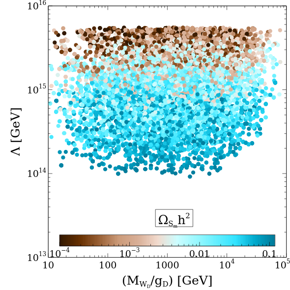
The LP of Fig. 12 shows the allowed region in the – plane where the colour represents the FIMP DM relic density. One may easily see that, for a fixed value of the FIMP DM mass, increasing the value of makes the FIMP contribution to DM relic density decrease, as the FIMP DM production is inversely proportional to . The lower limit in the value comes from the maximum allowed range for DM relic density, , since the relic density is proportional to . In the RP of Fig. 12, we present the allowed range in the – plane. One may again observe that, as we go to a higher value of , we have a smaller FIMP DM contribution. The VEV linearly contributes to the FIMP DM relic density, and thus, for a higher value of , we need a higher value of to get the correct DM relic density value; we notice this in particular in the region and . This correlation between and is observed for higher values of , whereas we do not see such a correlation for lower values of . In both the LP and RP of Fig. 12, we see that there is no upper bound on . This is because such higher values of reduce the FIMP DM relic density, and the DM relic density bound can be satisfied from the contribution of the WIMP DM.


The LP of Fig. 13 shows the allowed range in the – plane after imposing . It is clearly shown in the figure that, to obtain the WIMP DM relic density below 0.12, we need to stay near the resonance region, i.e., . It is also clear that, when we are very close to the resonance region, we have a smaller WIMP contribution in the DM relic density, while a larger WIMP contribution is obtained as we depart from the resonance region. Moreover, we see that, for GeV, the dark Higgs mass may take any value. This is due to the fact that the dominating contribution comes from the SM Higgs resonance. The RP of Fig. 13 shows the allowed region in the – plane after imposing . One may see from the figure that, if we increase the value of , one may have a smaller contribution of WIMP DM. This happens because the annihilation cross section increases with , and the WIMP DM relic density is inversely proportional to annihilation cross section. For higher values of , we see no allowed point in the range as the region has a dominating FIMP DM contribution due to the high value of the VEV .
How close one needs to be to the resonance region is studied in Fig. 14 where the WIMP DM relic density is shown in terms of the mixing angle and . The parameter quantifies the closeness to the resonance region, and corresponds to the exact resonance point. We find that typically takes a value between and , depending on the value of the mixing angle, if we ask for the WIMP DM component to be a significant part of the total relic density. We observe that the window for a WIMP DM relic density of at least of the total DM relic density is narrower for smaller values of the mixing angle. At a fixed value of , the relic density decreases as the value of increases. One may understand this as follows: The process keeping the WIMP DM in thermal equilibrium is , and it is mediated by . We thus find that the cross section is proportional to . Higher values of mean being closer to the resonant point where the cross section increases. Therefore, the relic density decreases following the standard behaviour, . Once we depart too much from the resonance region, we may overproduce the WIMP DM and overclose the Universe.


Figure 15 shows the allowed region in the – (LP) and – (RP) planes, together with various direct and indirect detection bounds that are depicted by solid lines. Note that we have rescaled the -axes by the amount of the WIMP DM relic density compared to the total DM in the Universe . The LP of Fig. 15 may be easily understood with the direct detection expression given by Eq. (29), which states that is proportional to . One may estimate the percentage of the WIMP DM relic that each sample point corresponds to with the help of the RP of Fig. 13. Comparing the LP of Fig. 15 and RP of Fig. 13, one can easily see that lower values of correspond to lower values of and higher values of the WIMP DM relic density as the density is inversely proportional to . A sharp dip at GeV happens because of the mutual cancellation between the SM Higgs- and the BSM Higgs-mediated processes as one may see from Eq. 29. A part of the GeV region is already ruled out by the different direct detection experiments such as XENON-1T XENON:2018voc, PandaX-4T PandaX-II:2017hlx; Liu:2022zgu, and LUX-ZEPLIN-5.5T LZ:2022ufs. The region of DM mass below 7 GeV will be explored by DarkSide-50 DarkSide:2018kuk; DarkSide:2018bpj, XENON-1T(M) Ibe:2017yqa, CDMSlite SuperCDMS:2018gro, and CRESST-III CRESST:2017ues; CRESST:2019jnq. The black solid line corresponds to the bound from the Higgs invisible decay which is obtained by staying near the dark Higgs resonance region, i.e., , so that the WIMP DM never becomes over-abundant. The region above the black solid line is already ruled out by the current bound on the branching of the Higgs invisible decay mode. We note that our model predicts much lower values for compared to the aforementioned bounds. From the RP of Fig. 15, we see that there is a dip in for the WIMP DM mass below 5 GeV. This is due to the fact that, for this range, the channel is not active. The region of GeV is constrained by the Fermi-LAT + MAGIC Segue 1 data MAGIC:2016xys. We observe that most of the parameter space which contributes dominantly to the DM relic is already ruled out by the indirect detection bound. We have also checked the present bounds on the DM annihilation to and , and we present the results in Appendix D.
5 First-order phase transitions and associated gravitational waves
The extra dark Higgs field not only gives a mass to the WIMP DM , but it also changes the vacuum evolution. We study the evolution of the vacuum state and the dynamics of the phase transition in this section. We first compute the one-loop finite-temperature effective potential,
| (40) |
where is the tree-level scalar potential, is the one-loop Coleman-Weinberg potential, and is the finite-temperature correction. In terms of the background fields and of the SM Higgs and the dark Higgs, the tree-level scalar potential is given by
| (41) |
The Coleman-Weinberg potential can generically be written as
| (42) |
where the () sign is for bosons (fermions), is the number of degrees of freedom of the species , is the field-dependent mass, the constants are 1/2 for transverse gauge bosons and 2/3 for the rest, and is the renormalisation scale. The expressions for the field-dependent masses and are summarised in Appendix E. Depending on the choice of the renormalisation scale , the effective potential changes, and hence one may arrive at different results. This renormalisation scale dependence has been explored in e.g. Refs. Chiang:2018gsn; Croon:2020cgk44 4 See also e.g. Refs. Nielsen:1975fs; Fukuda:1975di; Patel:2011th; Chiang:2017zbz; Chiang:2018gsn; Croon:2020cgk; Schicho:2022wty for the gauge dependence issue. . Together with the gauge dependence issue, we do not attempt to address the issue of the renormalisation scale dependence as it goes beyond the scope of the current work. We thus ignore the one-loop Coleman-Weinberg corrections in the followings by assuming that the renormalisation scale is chosen in such a way that the Coleman-Weinberg corrections are minimised. The finite-temperature correction is given by Dolan:1973qd
| (43) |
with
| (44) |
where is for bosons and is for fermions. The re-summed ring diagrams are taken into account by replacing the field-dependent masses as Parwani:1991gq
| (45) |
where are the thermal masses Carrington:1991hz. We present the thermal mass expressions in Appendix F. Up to the leading order, the effective potential is thus given by
| (46) |
where and ‘’ include sub-leading, negligible terms. Note that we have assumed that the dark gauge coupling is small enough not to affect the leading-order terms.
In the presence of the extra Higgs field, FOPTs may arise. FOPTs with a dark have been studied in e.g. Refs. Chao:2014ina; Hashino:2018zsi; Breitbach:2018ddu; Borah:2021ocu. For studies of the phase transition with an extra scalar field, see, e.g., Refs. Cline:2012hg; Vaskonen:2016yiu; Kurup:2017dzf; Chiang:2018gsn; Ellis:2018mja; Carena:2019une; Biondini:2022ggt; Schicho:2022wty. In particular, in Ref. Carena:2019une where the studied scalar potential has the same form as Eq. (46), it was shown both analytically and numerically that the FOPTs could be strong, characterised by . Here, is the critical temperature at which the potential minima become degenerate, and is the VEV of the SM Higgs field at . It indicates that one of the Sakharov conditions for successful electroweak baryogenesis can be fulfilled Sakharov:1967dj. Since the scalar field space is now two-dimensional due to the extra Higgs field, one may achieve either one-step or two-step phase transitions. Noting that the VEV of the Higgs is non-zero at zero temperature, the one-step phase transition has the pattern , while the two-step phase transition may occur via or . For the two-step phase transition of the pattern , the second step breaks the electroweak symmetry, giving Carena:2019une
| (47) |
One may see that strongly FOPTs, , can be achieved when the dark Higgs is lighter than the SM Higgs. The one-step phase transition shows a similar behaviour Carena:2019une. Utilising the publicly available tool CosmoTransitions Wainwright:2011kj, we numerically compute for a wide range of the parameter space and present the result in Fig. 16. The explored parameter range is as follows:
| (48) |
We note that these four input parameters are the only relevant model parameters. The other model parameters can be derived from the above input parameters. The -axis of Fig. 16 is defined as . We observe that strong FOPTs could be achieved for small values of , which is in good agreement with both the analytical estimate (47) and the results of Ref. Carena:2019une.
FOPTs may produce observable stochastic GWs Kamionkowski:1993fg. There are three main contributions to the GWs from the FOPT: bubble wall collisions , sound wave in plasma , and the magneto-hybrodynamic turbulence . The total GWs are then . The GWs coming from the bubble wall collisions are given by Caprini:2015zlo
| (49) |
while the turbulence contribution is Caprini:2015zlo
| (50) |
where
| (51) |
Finally, the sound-wave contribution to the GW signal can be expressed as Ellis:2018mja; Ellis:2019oqb; Ellis:2020awk; Guo:2020grp
| (52) |
For the expressions for , , , , , , and , see Appendix G.
Three parameters that play the key roles in the GW signal are
| (53) |
where is the Euclidean action of a bubble with being the three-dimensional action, the released energy density during the phase transition, and , with being the number of effective degrees of freedom at . We take to be the nucleation temperature . We employ CosmoTransitions Wainwright:2011kj to numerically compute the three key parameters, , , and the nucleation temperature . In Fig. 17, we present the FOPT-associated GW signals for three BPs together with the sensitivity curves of future space-based GW experiments such as LISA, DECIGO, and BBO. The three BPs, that account for not only the neutrino masses and the correct DM relic density, but also the strong FOPTs, are summarised in Table 2. One may notice that the three BPs have different DM compositions. In the case of the first BP (BP1), both the WIMP and FIMP contribute equally to the total DM relic density, while the BP2 (BP3) is mostly composed of the FIMP (WIMP) DM. We see from Fig. 17 that the GW signals for all the BPs are well within the reach of the detectability threshold of BBO, DECIGO, and Ultimate-DECIGO.
| BPs | [TeV] | [GeV] | [] | [GeV] | ||||||
|---|---|---|---|---|---|---|---|---|---|---|
| BP1 | 3.37 | 2.21 | 0.082 | 3.1 | 0.238 | 13671 | 34.43 | 4.67 | 0.46 | 0.54 |
| BP2 | 0.673 | 2.77 | -0.076 | 19.7 | 0.139 | 6760.0 | 46.67 | 3.56 | 0.044 | 0.956 |
| BP3 | 4.63 | 1.0 | 0.060 | 1.0 | 0.461 | 13820 | 21.58 | 6.76 | 0.87 | 0.13 |
6 Collider Searches
The present work deals with the WIMP and FIMP-type DMs. Due to the feeble interaction of the FIMP, it is difficult to probe it at collider experiments. We can, however, focus on general search strategies for BSM particles in the context of the present work. In particular, we may study the production of the second Higgs at the or colliders and look for its subsequent decay. Suitably adjusting the WIMP DM mass allows the second Higgs to decay mainly to the WIMP DM, and we may look for the missing energy with mono-jet or di-jet signals in the final state. Otherwise, if does not dominantly decay to the WIMP DM, then it will decay to the SM particles such as the SM Higgs. See, e.g., Refs. Banerjee:2015gca; Belanger:2021slj. The relevant signal channels for our current study at the collider would be
| (54) |
where corresponds to the initial or final state jets, is associated with the SM lepton, and is the transverse missing energy. Similar to the SM Higgs searches, we can also investigate
| (55) |
at the collider. The exact values of the integers, , , and , depend on the production cross section and dominance of the associated backgrounds. Moreover, exploring the singlet fermions () of our model at different colliders is an interesting direction; see, e.g., Ref. Banerjee:2015gca. Further comments require a full-fledged collider study which is out of the scope of the current work, and we leave it for future study.
7 Conclusion
We have studied an extension of the Standard Model that accounts for the dark matter and the smallness of the neutrino masses under the extended seesaw framework. In our model, two sets of three-generation neutrinos are introduced; the first two generations provide the light neutrinos with a mass, and the third-generation neutrinos become FIMP-like particles. Amongst these FIMP-like particles, the heavier one eventually decays into the lighter one, and thus, we have the lighter third-generation neutrino as the FIMP dark matter candidate. Our model also contains a WIMP dark matter candidate, namely the dark gauge boson. Thus, a two-component WIMP-FIMP dark matter scenario naturally arises in our model.
We have explored allowed parameter spaces by using the lepton flavour violating bounds as well as the neutrino oscillation data. Much of the parameter spaces are already tightly constrained, but we have shown that there are viable parameter regions which are free from the constraints. Prospects of various future experiments have been discussed as well. Interestingly, the contribution to the FIMP dark matter relic density coming from neutrinos scattering is found to be up to a of the total relic density for the range of the model parameters considered in our study. We have also discussed the dependence of the relic density on the model parameters. Utilising publicly available tools, we have performed extensive numerical parameter scans in order to study the evolutions of the dark matter candidates. Parameter spaces compatible with the bounds from (in-)direct detection and collider searches are presented. In particular, we have showed regions where a two-component dark matter scenario is realised and testable by future (in-)direct experiments.
The dark Higgs field plays a major role in the FIMP and WIMP dark matter productions. In addition, the extra scalar field also changes the evolution of the vacuum state in the scalar sector, making a first-order phase transition possible. We have demonstrated that the strength of the electroweak first-order phase transition, quantified by the quantity , where is the critical temperature and is the SM Higgs vacuum expectation value at , may become larger than unity for small values of the dark Higgs mass. Therefore, one of the essential ingredients for a successful electroweak baryogenesis is achieved in our model. We have also studied stochastic gravitational waves associated with the first-order phase transitions and showed that the gravitational wave signals are strong enough to be detectable by future experiments such as BBO and DECIGO.
Three benchmark points, that explicitly demonstrate the capability of i) having a correct dark matter relic density, ii) generating the non-zero neutrino masses with the extended seesaw mechanism, iii) achieving a strongly first-order phase transition, and iv) emitting stochastic gravitational waves detectable by future experiments, are presented. Thus, the model studied in this work has an exciting potential detectability not only with future (in-)direct detection experiments and collider searches, but also with future gravitational wave experiments.
Acknowledgements.
J.K. would like to thank Yikun Wang for useful discussions on the phase transition and the use of CosmoTransitions. S.K. would like to acknowledge Geneviève Bélanger for the help related with micrOMEGAs. The work of F.C. is supported by the European Union’s Horizon 2020 research and innovation programme under the Marie Skłodowska-Curie grant agreement No 860881-HIDDeN. This work used the Scientific Compute Cluster at GWDG, the joint data center of Max Planck Society for the Advancement of Science (MPG) and University of Göttingen.Appendix A WIMP DM decay width through kinetic mixing
In the presence of the mixing between the WIMP DM and the gauge boson, the DM may decay to, e.g., electrons, through the coupling between the DM and SM fermions Biswas:2021dan. For simplicity, we consider the decay of the DM to electrons. The decay width is then given by
| (56) |
where , , is the fine-structure constant, is the weak angle, and is the gauge kinetic mixing parameter introduced in (1). Considering the DM mass of 10 GeV, and requiring the lifetime of the DM to be is larger than the age of the universe, we get an upper bound on the gauge kinetic mixing parameter as . When the decay of the DM to the SM fermions is open, the -ray observation may become relevant Fermi-LAT:2015kyq. In this case, the DM lifetime should be greater than s Fermi-LAT:2015kyq, which puts an even stronger bound of .
Appendix B Quartic couplings
The scalar quartic couplings may be written in terms of the mixing angle and masses of the physical Higgses as follows:
| (57) | ||||
Appendix C Feynman Diagrams
Figure 18 shows the diagrams which contribute to the processes , , and -to- conversion. We have considered these diagrams for the discussion of the LFV bounds.
The Feynman diagrams relevant for our DM analysis are shown in Fig. 19.
Appendix D DM annihilation to and


The LP and RP of Fig. 20 present the DM annihilation to and , respectively, together with the bounds from FERMI-LAT Fermi-LAT:2015att; Leane:2018kjk, CMB Leane:2018kjk, and AMS Bergstrom:2013jra; Leane:2018kjk data. We find that our model predicts orders of magnitude lower than the current bound. We expect that our model parameter space may be explored in future by different ongoing indirect detection experiments. Finally, we note that the DM annihilation to is many orders below than the current bound as well.
Appendix E Field-dependent masses
We summarise the expressions for the field-dependent masses as well as the number of degrees of freedom that appear in the one-loop Coleman-Weinberg potential (42):
and
Note that we have considered only the most dominant SM top quark for the fermionic states.
Appendix F Thermal masses
We summarise the expressions for the thermal masses that enter the one-loop temperature-dependent potential (43):
where we have considered only the most dominant SM top quark for the fermionic states. Note that fermions and transverse modes of the gauge bosons do not receive any thermal correction.
Appendix G Gravitational wave-related expressions
The quantities , , and that appear in , , and are given as follows Caprini:2015zlo:
The bubble wall velocity is given by Steinhardt:1981ct
and we adopt Kamionkowski:1993fg
References
- (1) T. S.-K. Collaboration and Y. F. et al, Evidence for oscillation of atmospheric neutrinos, Physical Review Letters 81 (1998) 1562 [hep-ex/9807003].
- (2) M. C. Gonzalez-Garcia and Y. Nir, Neutrino Masses and Mixing: Evidence and Implications, Reviews of Modern Physics 75 (2003) 345 [hep-ph/0202058].
- (3) I. Esteban, M. C. Gonzalez-Garcia, M. Maltoni, T. Schwetz and A. Zhou, The fate of hints: Updated global analysis of three-flavor neutrino oscillations, Journal of High Energy Physics 2020 (2020) 178 [2007.14792].
- (4) Planck collaboration, Planck 2015 results. XIII. Cosmological parameters, Astronomy & Astrophysics 594 (2016) A13 [1502.01589].
- (5) Planck collaboration, Planck 2018 results. VI. Cosmological parameters, Astronomy & Astrophysics 641 (2020) A6 [1807.06209].
- (6) P. Minkowski, e at a rate of one out of 109 muon decays?, Physics Letters B 67 (1977) 421.
- (7) M. Gell-Mann, P. Ramond and R. Slansky, Complex Spinors and Unified Theories, 1306.4669.
- (8) S. K. Kang and C. S. Kim, Extended double seesaw model for neutrino mass spectrum and low scale leptogenesis, Physics Letters B 646 (2007) 248 [hep-ph/0607072].
- (9) M. Mitra, G. Senjanovic and F. Vissani, Neutrinoless Double Beta Decay and Heavy Sterile Neutrinos, Nuclear Physics B 856 (2012) 26 [1108.0004].
- (10) S. K. Majee, M. K. Parida and A. Raychaudhuri, Neutrino mass and low-scale leptogenesis in a testable SUSY SO(10) model, 0807.3959.
- (11) M. Kawasaki, K. Kohri and T. Moroi, Big-Bang nucleosynthesis and hadronic decay of long-lived massive particles, Physical Review D: Particles and Fields 71 (2005) 083502 [astro-ph/0408426].
- (12) A. Hook, R. McGehee and H. Murayama, Cosmologically viable low-energy supersymmetry breaking, Physical Review D: Particles and Fields 98 (2018) 115036 [1801.10160].
- (13) J. P. Ostriker and P. J. E. Peebles, A Numerical Study of the Stability of Flattened Galaxies: Or, can Cold Galaxies Survive?, The Astrophysical Journal 186 (1973) 467.
- (14) E. Corbelli and P. Salucci, The Extended Rotation Curve and the Dark Matter Halo of M33, Monthly Notices of the Royal Astronomical Society 311 (2000) 441 [astro-ph/9909252].
- (15) J. E. Gunn, B. W. Lee, I. Lerche, D. N. Schramm and G. Steigman, Some astrophysical consequences of the existence of a heavy stable neutral lepton., The Astrophysical Journal 223 (1978) 1015.
- (16) P. Hut, Limits on masses and number of neutral weakly interacting particles, Physics Letters B 69 (1977) 85.
- (17) B. W. Lee and S. Weinberg, Cosmological Lower Bound on Heavy-Neutrino Masses, Physical Review Letters 39 (1977) 165.
- (18) G. Bertone, D. Hooper and J. Silk, Particle dark matter: Evidence, candidates and constraints, Physics Reports 405 (2005) 279 [hep-ph/0404175].
- (19) XENON collaboration, Dark Matter Search Results from a One Ton-Year Exposure of XENON1T, Physical Review Letters 121 (2018) 111302 [1805.12562].
- (20) CMS collaboration, Phenomenological MSSM interpretation of CMS searches in pp collisions at sqrt(s) = 7 and 8 TeV, Journal of High Energy Physics 10 (2016) 129 [1606.03577].
- (21) MAGIC, Fermi-LAT collaboration, Limits to dark matter annihilation cross-section from a combined analysis of MAGIC and Fermi-LAT observations of dwarf satellite galaxies, Journal of Cosmology and Astroparticle Physics 02 (2016) 039 [1601.06590].
- (22) G. Arcadi, M. Dutra, P. Ghosh, M. Lindner, Y. Mambrini, M. Pierre et al., The waning of the WIMP? A review of models, searches, and constraints, European Physical Journal C 78 (2018) 203 [1703.07364].
- (23) PandaX-II collaboration, Dark Matter Results from First 98.7 Days of Data from the PandaX-II Experiment, Physical Review Letters 117 (2016) 121303 [1607.07400].
- (24) LUX collaboration, Results from a Search for Dark Matter in the Complete LUX Exposure, Physical Review Letters 118 (2017) 021303 [1608.07648].
- (25) J. McDonald, Thermally Generated Gauge Singlet Scalars as Self-Interacting Dark Matter, Physical Review Letters 88 (2002) 091304 [hep-ph/0106249].
- (26) K.-Y. Choi and L. Roszkowski, E-WIMPs, hep-ph/0511003.
- (27) A. Kusenko, Sterile Neutrinos, Dark Matter, and Pulsar Velocities in Models with a Higgs Singlet, Physical Review Letters 97 (2006) 241301 [hep-ph/0609081].
- (28) L. J. Hall, K. Jedamzik, J. March-Russell and S. M. West, Freeze-in production of FIMP dark matter, Journal of High Energy Physics 03 (2010) 080 [0911.1120].
- (29) C. Cheung, G. Elor and L. Hall, Gravitino freeze-in, Physical Review D 84 (2011) 115021 [1103.4394].
- (30) F. Elahi, C. Kolda and J. Unwin, UltraViolet freeze-in, Journal of High Energy Physics 03 (2015) 048 [1410.6157].
- (31) G. Arcadi, L. Covi and M. Nardecchia, Gravitino dark matter and low-scale baryogenesis, Physical Review D 92 (2015) 115006 [1507.05584].
- (32) N. Bernal, M. Heikinheimo, T. Tenkanen, K. Tuominen and V. Vaskonen, The dawn of FIMP Dark Matter: A review of models and constraints, International Journal of Modern Physics A 32 (2017) 1730023 [1706.07442].
- (33) K. Benakli, Y. Chen, E. Dudas and Y. Mambrini, Minimal model of gravitino dark matter, Physical Review D 95 (2017) 095002 [1701.06574].
- (34) N. Bernal, M. Dutra, Y. Mambrini, K. Olive, M. Peloso and M. Pierre, Spin-2 portal dark matter, Physical Review D 97 (2018) 115020 [1803.01866].
- (35) N. Bernal, F. Elahi, C. Maldonado and J. Unwin, Ultraviolet Freeze-in and Non-Standard Cosmologies, Journal of Cosmology and Astroparticle Physics 11 (2019) 026 [1909.07992].
- (36) B. Barman, S. Bhattacharya and M. Zakeri, Non-abelian vector boson as FIMP dark matter, JCAP 02 (2020) 029 [1905.07236].
- (37) L. Covi, A. Ghosh, T. Mondal and B. Mukhopadhyaya, Models of decaying FIMP Dark Matter: Potential links with the Neutrino Sector, 2008.12550.
- (38) S. Khan, Explaining Xenon-1T signal with FIMP dark matter and neutrino mass in a U(1)X extension, The European Physical Journal C: Particles and Fields 81 (2021) 598 [2007.13008].
- (39) M. A. G. Garcia, Y. Mambrini, K. A. Olive and S. Verner, The case for decaying spin-3/2 dark matter, Physical Review D 102 (2020) 083533 [2006.03325].
- (40) N. Bernal, J. Rubio and H. Veermäe, UV Freeze-in in Starobinsky Inflation, Journal of Cosmology and Astroparticle Physics 10 (2020) 021 [2006.02442].
- (41) B. Barman, D. Borah and R. Roshan, Effective theory of freeze-in dark matter, JCAP 11 (2020) 021 [2007.08768].
- (42) B. Barman, S. Bhattacharya and B. Grzadkowski, Feebly coupled vector boson dark matter in effective theory, JHEP 12 (2020) 162 [2009.07438].
- (43) B. Barman, P. Ghosh, A. Ghoshal and L. Mukherjee, Shedding flavor on dark via freeze-in: U(1)B-3L i gauged extensions, JCAP 08 (2022) 049 [2112.12798].
- (44) B. Barman and A. Ghoshal, Scale invariant FIMP miracle, JCAP 03 (2022) 003 [2109.03259].
- (45) G. Bélanger, S. Khan, R. Padhan, M. Mitra and S. Shil, Right handed neutrinos, TeV scale BSM neutral Higgs boson, and FIMP dark matter in an EFT framework, Physical Review D: Particles and Fields 104 (2021) 055047 [2104.04373].
- (46) B. Barman and A. Ghoshal, Probing pre-BBN era with scale invarint FIMP, 2203.13269.
- (47) K. Choi and S. H. Im, Realizing the relaxion from multiple axions and its UV completion with high scale supersymmetry, JHEP 01 (2016) 149 [1511.00132].
- (48) D. E. Kaplan and R. Rattazzi, Large field excursions and approximate discrete symmetries from a clockwork axion, Physical Review D: Particles and Fields 93 (2016) 085007 [1511.01827].
- (49) G. F. Giudice and M. McCullough, A clockwork theory, JHEP 02 (2017) 036 [1610.07962].
- (50) J. Kim and J. McDonald, Clockwork Higgs portal model for freeze-in dark matter, Physical Review D: Particles and Fields 98 (2018) 023533 [1709.04105].
- (51) J. Kim and J. Mcdonald, Freeze-in dark matter from a sub-Higgs mass clockwork sector via the higgs portal, Physical Review D: Particles and Fields 98 (2018) 123503 [1804.02661].
- (52) A. Goudelis, K. A. Mohan and D. Sengupta, Clockworking FIMPs, JHEP 10 (2018) 014 [1807.06642].
- (53) K. M. Zurek, Multi-component dark matter, Physical Review D: Particles and Fields 79 (2009) 115002 [0811.4429].
- (54) S. Profumo, K. Sigurdson and L. Ubaldi, Can we discover multi-component WIMP dark matter?, JCAP 12 (2009) 016 [0907.4374].
- (55) D. Feldman, Z. Liu, P. Nath and G. Peim, Multicomponent dark matter in supersymmetric hidden sector extensions, Physical Review D: Particles and Fields 81 (2010) 095017 [1004.0649].
- (56) P. Ko and Y. Omura, Supersymmetric U(1)B X U(1)L model with leptophilic and leptophobic cold dark matters, Physics Letters B 701 (2011) 363 [1012.4679].
- (57) A. Drozd, B. Grzadkowski and J. Wudka, Multi-scalar-singlet extension of the standard model - the case for dark matter and an invisible higgs boson, JHEP 04 (2012) 006 [1112.2582].
- (58) M. Aoki, M. Duerr, J. Kubo and H. Takano, Multi-component dark matter systems and their observation prospects, Physical Review D: Particles and Fields 86 (2012) 076015 [1207.3318].
- (59) S. Bhattacharya, A. Drozd, B. Grzadkowski and J. Wudka, Two-component dark matter, JHEP 10 (2013) 158 [1309.2986].
- (60) S. Baek, P. Ko and W.-I. Park, Hidden sector monopole, vector dark matter and dark radiation with Higgs portal, JCAP 10 (2014) 067 [1311.1035].
- (61) S. Esch, M. Klasen and C. E. Yaguna, A minimal model for two-component dark matter, JHEP 09 (2014) 108 [1406.0617].
- (62) P. Ko and Y. Tang, MDM: A model for sterile neutrino and dark matter reconciles cosmological and neutrino oscillation data after BICEP2, Physics Letters B 739 (2014) 62 [1404.0236].
- (63) L. Bian, T. Li, J. Shu and X.-C. Wang, Two component dark matter with multi-Higgs portals, JHEP 03 (2015) 126 [1412.5443].
- (64) A. Karam and K. Tamvakis, Dark matter and neutrino masses from a scale-invariant multi-Higgs portal, Physical Review D: Particles and Fields 92 (2015) 075010 [1508.03031].
- (65) G. Arcadi, C. Gross, O. Lebedev, Y. Mambrini, S. Pokorski and T. Toma, Multicomponent dark matter from gauge symmetry, JHEP 12 (2016) 081 [1611.00365].
- (66) A. Dutta Banik, M. Pandey, D. Majumdar and A. Biswas, Two component WIMP–FImP dark matter model with singlet fermion, scalar and pseudo scalar, The European Physical Journal C: Particles and Fields 77 (2017) 657 [1612.08621].
- (67) A. Karam and K. Tamvakis, Dark matter from a classically scale-invariant SU(3)X, Physical Review D: Particles and Fields 94 (2016) 055004 [1607.01001].
- (68) S. Bhattacharya, P. Poulose and P. Ghosh, Multipartite interacting scalar dark matter in the light of updated LUX data, JCAP 04 (2017) 043 [1607.08461].
- (69) P. Ko and Y. Tang, Residual non-abelian dark matter and dark radiation, Physics Letters B 768 (2017) 12 [1609.02307].
- (70) M. Aoki and T. Toma, Implications of two-component dark matter induced by forbidden channels and thermal freeze-out, JCAP 01 (2017) 042 [1611.06746].
- (71) A. Ahmed, M. Duch, B. Grzadkowski and M. Iglicki, Multi-Component Dark Matter: The vector and fermion case, The European Physical Journal C: Particles and Fields 78 (2018) 905 [1710.01853].
- (72) M. Aoki and T. Toma, Boosted self-interacting dark matter in a multi-component dark matter model, JCAP 10 (2018) 020 [1806.09154].
- (73) S. Chakraborti and P. Poulose, Interplay of scalar and fermionic components in a multi-component dark matter scenario, The European Physical Journal C: Particles and Fields 79 (2019) 420 [1808.01979].
- (74) A. Poulin and S. Godfrey, Multicomponent dark matter from a hidden gauged SU(3), Physical Review D: Particles and Fields 99 (2019) 076008 [1808.04901].
- (75) S. Yaser Ayazi and A. Mohamadnejad, Scale-invariant two component dark matter, The European Physical Journal C: Particles and Fields 79 (2019) 140 [1808.08706].
- (76) S. Chakraborti, A. Dutta Banik and R. Islam, Probing multicomponent extension of inert doublet model with a vector dark matter, The European Physical Journal C: Particles and Fields 79 (2019) 662 [1810.05595].
- (77) S. Bhattacharya, P. Ghosh, A. K. Saha and A. Sil, Two component dark matter with inert Higgs doublet: Neutrino mass, high scale validity and collider searches, JHEP 03 (2020) 090 [1905.12583].
- (78) C.-R. Chen, Y.-X. Lin, C. S. Nugroho, R. Ramos, Y.-L. S. Tsai and T.-C. Yuan, Complex scalar dark matter in the gauged two-Higgs-doublet model, Physical Review D: Particles and Fields 101 (2020) 035037 [1910.13138].
- (79) C. E. Yaguna and Ó. Zapata, Multi-component scalar dark matter from a ZN symmetry: A systematic analysis, JHEP 03 (2020) 109 [1911.05515].
- (80) S. Bhattacharya, N. Chakrabarty, R. Roshan and A. Sil, Multicomponent dark matter in extended U(1)B-L: Neutrino mass and high scale validity, JCAP 04 (2020) 013 [1910.00612].
- (81) A. Betancur, G. Palacio and A. Rivera, Inert doublet as multicomponent dark matter, Nuclear Physics B 962 (2021) 115276 [2002.02036].
- (82) G. Bélanger, A. Pukhov, C. E. Yaguna and Ó. Zapata, The Z5 model of two-component dark matter, JHEP 09 (2020) 030 [2006.14922].
- (83) G. Belanger, A. Mjallal and A. Pukhov, Two dark matter candidates: The case of inert doublet and singlet scalars, Physical Review D: Particles and Fields 105 (2022) 035018 [2108.08061].
- (84) S. Bhattacharya, S. Chakraborti and D. Pradhan, Electroweak symmetry breaking and WIMP-FIMP dark matter, JHEP 07 (2022) 091 [2110.06985].
- (85) P. Das, M. K. Das and N. Khan, The FIMP-WIMP dark matter in the extended singlet scalar model, Nuclear Physics B 975 (2022) 115677 [2104.03271].
- (86) A. Betancur, A. Castillo, G. Palacio and J. Suarez, Multicomponent scalar dark matter at high-intensity proton beam experiments, Journal of Physics G: Nuclear and Particle Physics 49 (2022) 075003 [2109.11586].
- (87) N. Chakrabarty, R. Roshan and A. Sil, Two-component doublet-triplet scalar dark matter stabilizing the electroweak vacuum, Physical Review D: Particles and Fields 105 (2022) 115010 [2102.06032].
- (88) A. Mohamadnejad, Electroweak phase transition and gravitational waves in a two-component dark matter model, Journal of High Energy Physics 03 (2022) 188 [2111.04342].
- (89) B. Díaz Sáez, K. Möhling and D. Stöckinger, Two real scalar WIMP model in the assisted freeze-out scenario, JCAP 10 (2021) 027 [2103.17064].
- (90) S.-M. Choi, J. Kim, P. Ko and J. Li, A multi-component SIMP model with U(1)X→ Z2 × Z3, JHEP 09 (2021) 028 [2103.05956].
- (91) G. Belanger, A. Mjallal and A. Pukhov, WIMP and FIMP dark matter in the inert doublet plus singlet model, 2205.04101.
- (92) A. Das, S. Gola, S. Mandal and N. Sinha, Two-component scalar and fermionic dark matter candidates in a generic U(1)X model, Physics Letters B 829 (2022) 137117 [2202.01443].
- (93) S.-Y. Ho, P. Ko and C.-T. Lu, Scalar and fermion two-component SIMP dark matter with an accidental Z4 symmetry, JHEP 03 (2022) 005 [2201.06856].
- (94) F. Costa, S. Khan and J. Kim, A Two-Component Dark Matter Model and its Associated Gravitational Waves, Journal of High Energy Physics 06 (2022) 026 [2202.13126].
- (95) M. Kamionkowski, A. Kosowsky and M. S. Turner, Gravitational Radiation from First-Order Phase Transitions, Physical Review D 49 (1994) 2837 [astro-ph/9310044].
- (96) J. Baker, J. Bellovary, P. L. Bender, E. Berti, R. Caldwell, J. Camp et al., The Laser Interferometer Space Antenna: Unveiling the Millihertz Gravitational Wave Sky, 1907.06482.
- (97) N. Seto, S. Kawamura and T. Nakamura, Possibility of Direct Measurement of the Acceleration of the Universe Using 0.1 Hz Band Laser Interferometer Gravitational Wave Antenna in Space, Physical Review Letters 87 (2001) 221103 [astro-ph/0108011].
- (98) S. Kawamura, T. Nakamura, M. Ando, N. Seto, K. Tsubono, K. Numata et al., The Japanese space gravitational wave antenna—DECIGO, Classical and Quantum Gravity 23 (2006) S125.
- (99) S. Sato, S. Kawamura, M. Ando, T. Nakamura, K. Tsubono, A. Araya et al., The status of DECIGO, Journal of Physics: Conference Series 840 (2017) 012010.
- (100) S. Isoyama, H. Nakano and T. Nakamura, Multiband Gravitational-Wave Astronomy: Observing binary inspirals with a decihertz detector, B-DECIGO, Progress of Theoretical and Experimental Physics 2018 (2018) 073E01 [1802.06977].
- (101) S. Kawamura, M. Ando, N. Seto, S. Sato, M. Musha, I. Kawano et al., Current status of space gravitational wave antenna DECIGO and B-DECIGO, 2006.13545.
- (102) V. Corbin and N. J. Cornish, Detecting the Cosmic Gravitational Wave Background with the Big Bang Observer, Classical and Quantum Gravity 23 (2006) 2435 [gr-qc/0512039].
- (103) J. Crowder and N. J. Cornish, Beyond LISA: Exploring Future Gravitational Wave Missions, Physical Review D 72 (2005) 083005 [gr-qc/0506015].
- (104) G. M. Harry, P. Fritschel, D. A. Shaddock, W. Folkner and E. S. Phinney, Laser interferometry for the Big Bang Observer, Classical and Quantum Gravity 23 (2006) 4887.
- (105) C. Grojean and G. Servant, Gravitational Waves from Phase Transitions at the Electroweak Scale and Beyond, Physical Review D 75 (2007) 043507 [hep-ph/0607107].
- (106) S. J. Huber and T. Konstandin, Gravitational Wave Production by Collisions: More Bubbles, Journal of Cosmology and Astroparticle Physics 09 (2008) 022 [0806.1828].
- (107) J. R. Espinosa, T. Konstandin, J. M. No and M. Quiros, Some Cosmological Implications of Hidden Sectors, Physical Review D 78 (2008) 123528 [0809.3215].
- (108) C. Caprini, M. Hindmarsh, S. Huber, T. Konstandin, J. Kozaczuk, G. Nardini et al., Science with the space-based interferometer eLISA. II: Gravitational waves from cosmological phase transitions, Journal of Cosmology and Astroparticle Physics 04 (2016) 001 [1512.06239].
- (109) M. Artymowski, M. Lewicki and J. D. Wells, Gravitational wave and collider implications of electroweak baryogenesis aided by non-standard cosmology, Journal of High Energy Physics 03 (2017) 066 [1609.07143].
- (110) I. Baldes, Gravitational waves from the asymmetric-dark-matter generating phase transition, Journal of Cosmology and Astroparticle Physics 05 (2017) 028 [1702.02117].
- (111) A. Beniwal, M. Lewicki, M. White and A. G. Williams, Gravitational waves and electroweak baryogenesis in a global study of the extended scalar singlet model, Journal of High Energy Physics 02 (2019) 183 [1810.02380].
- (112) K. Hashino, M. Kakizaki, S. Kanemura, P. Ko and T. Matsui, Gravitational waves from first order electroweak phase transition in models with the U(1)X gauge symmetry, JHEP 06 (2018) 088 [1802.02947].
- (113) C. Caprini and D. G. Figueroa, Cosmological Backgrounds of Gravitational Waves, Classical and Quantum Gravity 35 (2018) 163001 [1801.04268].
- (114) L. Bian and Y.-L. Tang, Thermally modified sterile neutrino portal dark matter and gravitational waves from phase transition: The Freeze-in case, Journal of High Energy Physics 12 (2018) 006 [1810.03172].
- (115) L. Bian and X. Liu, Two-step strongly first-order electroweak phase transition modified FIMP dark matter, gravitational wave signals, and the neutrino mass, Physical Review D 99 (2019) 055003 [1811.03279].
- (116) L. Bian, W. Cheng, H.-K. Guo and Y. Zhang, Cosmological implications of a B - L charged hidden scalar: Leptogenesis and gravitational waves, Chinese Physics C 45 (2021) 113104 [1907.13589].
- (117) L. Bian, Y. Wu and K.-P. Xie, Electroweak phase transition with composite Higgs models: Calculability, gravitational waves and collider searches, Journal of High Energy Physics 12 (2019) 028 [1909.02014].
- (118) C. Caprini, M. Chala, G. C. Dorsch, M. Hindmarsh, S. J. Huber, T. Konstandin et al., Detecting gravitational waves from cosmological phase transitions with LISA: An update, Journal of Cosmology and Astroparticle Physics 03 (2020) 024 [1910.13125].
- (119) Y. Di, J. Wang, R. Zhou, L. Bian, R.-G. Cai and J. Liu, Magnetic field and gravitational waves from the first-order Phase Transition, Physical Review Letters 126 (2021) 251102 [2012.15625].
- (120) R. Zhou, L. Bian and J. Shu, Probing new physics for (g-2) and gravitational waves, 2104.03519.
- (121) L. Bian, Y.-L. Tang and R. Zhou, FIMP dark matter mediated by massive gauge boson around the phase transition period and the gravitational waves production, 2111.10608.
- (122) W. Altmannshofer, S. Gori, J. Martín-Albo, A. Sousa and M. Wallbank, Neutrino tridents at DUNE, Physical Review D: Particles and Fields 100 (2019) 115029 [1902.06765].
- (123) A. Biswas and S. Khan, (g - 2)e, and strongly interacting dark matter with collider implications, JHEP 07 (2022) 037 [2112.08393].
- (124) M. Bauer, P. Foldenauer and J. Jaeckel, Hunting all the hidden photons, JHEP 07 (2018) 094 [1803.05466].
- (125) Fermi-LAT collaboration, Updated search for spectral lines from galactic dark matter interactions with pass 8 data from the fermi large area telescope, Phys. Rev. D 91 (2015) 122002 [1506.00013].
- (126) B. Pontecorvo, Inverse beta processes and nonconservation of lepton charge, Zhurnal Eksperimental’noi i Teoreticheskoi Fiziki 7 (1958) 172.
- (127) Z. Maki, M. Nakagawa and S. Sakata, Remarks on the unified model of elementary particles, Progress of Theoretical Physics 28 (1962) 870.
- (128) MEG collaboration, Search for the lepton flavour violating decay →e+ with the full dataset of the MEG experiment, The European Physical Journal C: Particles and Fields 76 (2016) 434 [1605.05081].
- (129) SINDRUM collaboration, Search for the decay + → e+e+e-, Nuclear Physics B 299 (1988) 1.
- (130) P. Wintz, Results of the SINDRUM-II experiment, Conf. Proc. C 980420 (1998) 534.
- (131) A. Ilakovac and A. Pilaftsis, Flavour-Violating Charged Lepton Decays in Seesaw-Type Models, hep-ph/9403398.
- (132) M. Lindner, M. Platscher and F. S. Queiroz, A Call for New Physics : The Muon Anomalous Magnetic Moment and Lepton Flavor Violation, 1610.06587.
- (133) CHARM collaboration, A search for decays of heavy neutrinos in the mass range 0.5–2.8 GeV, Physics Letters B 166 (1986) 473.
- (134) CHARM II collaboration, Search for heavy isosinglet neutrinos, Physics Letters B 343 (1995) 453.
- (135) Belle collaboration, Search for heavy neutrinos at Belle, 1301.1105.
- (136) DELPHI collaboration, Search for neutral heavy leptons produced in Z decays, Zeitschrift für Physik 74 (1997) 57.
- (137) I. Krasnov, On DUNE prospects in the search for sterile neutrinos, Physical Review D 100 (2019) 075023 [1902.06099].
- (138) P. Ballett, T. Boschi and S. Pascoli, Heavy Neutral Leptons from low-scale seesaws at the DUNE Near Detector, Journal of High Energy Physics 03 (2020) 111 [1905.00284].
- (139) SHiP collaboration, Sensitivity of the SHiP experiment to Heavy Neutral Leptons, 1811.00930.
- (140) J. P. Chou, D. Curtin and H. J. Lubatti, New Detectors to Explore the Lifetime Frontier, Physics Letters B 767 (2017) 29 [1606.06298].
- (141) E. J. Chun, A. Das, S. Mandal, M. Mitra and N. Sinha, Sensitivity of Lepton Number Violating Meson Decays in Different Experiments, Physical Review D 100 (2019) 095022 [1908.09562].
- (142) FCC-ee study Team collaboration, Search for Heavy Right Handed Neutrinos at the FCC-ee, 1411.5230.
- (143) J. Alimena, P. Azzi, M. Bauer, A. Blondel, M. Drewes, R. G. Suarez et al., Searches for Long-Lived Particles at the Future FCC-ee, 2203.05502.
- (144) M. Drewes and J. Hajer, Heavy Neutrinos in displaced vertex searches at the LHC and HL-LHC, Journal of High Energy Physics 02 (2020) 070 [1903.06100].
- (145) S. Antusch, E. Cazzato and O. Fischer, Sterile neutrino searches via displaced vertices at LHCb, Physics Letters B 774 (2017) 114 [1706.05990].
- (146) NuTeV, E815 collaboration, Search for Neutral Heavy Leptons in a High-Energy Neutrino Beam, Physical Review Letters 83 (1999) 4943 [hep-ex/9908011].
- (147) FMMF collaboration, Search for neutral weakly interacting massive particles in the Fermilab Tevatron wideband neutrino beam, Physical Review D 52 (1995) 6.
- (148) J. L. Feng, I. Galon, F. Kling and S. Trojanowski, FASER: ForwArd Search ExpeRiment at the LHC, Physical Review D 97 (2018) 035001 [1708.09389].
- (149) D. Dercks, H. K. Dreiner, M. Hirsch and Z. S. Wang, Long-Lived Fermions at AL3X, Physical Review D 99 (2019) 055020 [1811.01995].
- (150) A. Alloul, N. D. Christensen, C. Degrande, C. Duhr and B. Fuks, FeynRules 2.0 - A complete toolbox for tree-level phenomenology, Computer Physics Communications 185 (2014) 2250 [1310.1921].
- (151) A. Belyaev, N. D. Christensen and A. Pukhov, CalcHEP 3.4 for collider physics within and beyond the Standard Model, Computer Physics Communications 184 (2013) 1729 [1207.6082].
- (152) G. Belanger, F. Boudjema, A. Pukhov and A. Semenov, micrOMEGAs2.0: A program to calculate the relic density of dark matter in a generic model, Computer Physics Communications 176 (2007) 367 [hep-ph/0607059].
- (153) M. Carena, Z. Liu and Y. Wang, Electroweak phase transition with spontaneous Z2-breaking, JHEP 08 (2020) 107 [1911.10206].
- (154) CMS collaboration, Combined measurements of Higgs boson couplings in proton–proton collisions at s=13 TeV , The European Physical Journal C: Particles and Fields 79 (2019) 421 [1809.10733].
- (155) ATLAS, CMS collaboration, Measurements of the Higgs boson production and decay rates and constraints on its couplings from a combined ATLAS and CMS analysis of the LHC pp collision data at s=7 and 8 TeV, JHEP 08 (2016) 045 [1606.02266].
- (156) A. Berlin, D. Hooper and S. D. McDermott, Simplified Dark Matter Models for the Galactic Center Gamma-Ray Excess, Physical Review D 89 (2014) 115022 [1404.0022].
- (157) P. Junnarkar and A. Walker-Loud, The Scalar Strange Content of the Nucleon from Lattice QCD, Physical Review D 87 (2013) 114510 [1301.1114].
- (158) LZ collaboration, First Dark Matter Search Results from the LUX-ZEPLIN (LZ) Experiment, 2207.03764.
- (159) PandaX-II collaboration, Dark Matter Results From 54-Ton-Day Exposure of PandaX-II Experiment, Physical Review Letters 119 (2017) 181302 [1708.06917].
- (160) PandaX collaboration, The first results of PandaX-4T, International Journal of Modern Physics D 31 (2022) 2230007.
- (161) DarkSide collaboration, DarkSide-50 532-day Dark Matter Search with Low-Radioactivity Argon, Physical Review D 98 (2018) 102006 [1802.07198].
- (162) DarkSide collaboration, Low-Mass Dark Matter Search with the DarkSide-50 Experiment, Physical Review Letters 121 (2018) 081307 [1802.06994].
- (163) M. Ibe, W. Nakano, Y. Shoji and K. Suzuki, Migdal Effect in Dark Matter Direct Detection Experiments, Journal of High Energy Physics 03 (2018) 194 [1707.07258].
- (164) SuperCDMS collaboration, Search for Low-Mass Dark Matter with CDMSlite Using a Profile Likelihood Fit, Physical Review D 99 (2019) 062001 [1808.09098].
- (165) CRESST collaboration, Results on MeV-scale dark matter from a gram-scale cryogenic calorimeter operated above ground, The European Physical Journal C 77 (2017) 637 [1707.06749].
- (166) CRESST collaboration, First results from the CRESST-III low-mass dark matter program, Physical Review D 100 (2019) 102002 [1904.00498].
- (167) Fermi-LAT collaboration, Searching for Dark Matter Annihilation from Milky Way Dwarf Spheroidal Galaxies with Six Years of Fermi-LAT Data, Physical Review Letters 115 (2015) 231301 [1503.02641].
- (168) R. K. Leane, T. R. Slatyer, J. F. Beacom and K. C. Y. Ng, GeV-Scale Thermal WIMPs: Not Even Slightly Dead, Physical Review D 98 (2018) 023016 [1805.10305].
- (169) L. Bergstrom, T. Bringmann, I. Cholis, D. Hooper and C. Weniger, New limits on dark matter annihilation from AMS cosmic ray positron data, Physical Review Letters 111 (2013) 171101 [1306.3983].
- (170) ATLAS collaboration, Combination of searches for invisible Higgs boson decays with the ATLAS experiment, Physical Review Letters 122 (2019) 231801 [1904.05105].
- (171) L. Covi, J. E. Kim and L. Roszkowski, Axinos as cold dark matter, Phys. Rev. Lett. 82 (1999) 4180 [hep-ph/9905212].
- (172) C.-W. Chiang, Y.-T. Li and E. Senaha, Revisiting electroweak phase transition in the standard model with a real singlet scalar, Physics Letters B 789 (2019) 154 [1808.01098].
- (173) D. Croon, O. Gould, P. Schicho, T. V. I. Tenkanen and G. White, Theoretical uncertainties for cosmological first-order phase transitions, JHEP 04 (2021) 055 [2009.10080].
- (174) N. K. Nielsen, On the gauge dependence of spontaneous symmetry breaking in gauge theories, Nuclear Physics B 101 (1975) 173.
- (175) R. Fukuda and T. Kugo, Gauge invariance in the effective action and potential, Physical Review D: Particles and Fields 13 (1976) 3469.
- (176) H. H. Patel and M. J. Ramsey-Musolf, Baryon Washout, Electroweak Phase Transition, and Perturbation Theory, Journal of High Energy Physics 07 (2011) 029 [1101.4665].
- (177) C.-W. Chiang and E. Senaha, On gauge dependence of gravitational waves from a first-order phase transition in classical scale-invariant U(1)’ models, Physics Letters B 774 (2017) 489 [1707.06765].
- (178) P. Schicho, T. V. I. Tenkanen and G. White, Combining thermal resummation and gauge invariance for electroweak phase transition, 2203.04284.
- (179) L. Dolan and R. Jackiw, Symmetry behavior at finite temperature, Physical Review D 9 (1974) 3320.
- (180) R. R. Parwani, Resummation in a hot scalar field theory, Physical Review D 45 (1992) 4695 [hep-ph/9204216].
- (181) M. E. Carrington, Effective potential at finite temperature in the standard model, Physical Review D 45 (1992) 2933.
- (182) W. Chao, First order electroweak phase transition triggered by the Higgs portal vector dark matter, Physical Review D: Particles and Fields 92 (2015) 015025 [1412.3823].
- (183) M. Breitbach, J. Kopp, E. Madge, T. Opferkuch and P. Schwaller, Dark, cold, and noisy: Constraining secluded hidden sectors with gravitational waves, JCAP 07 (2019) 007 [1811.11175].
- (184) D. Borah, A. Dasgupta and S. K. Kang, Gravitational waves from a dark U(1)D phase transition in light of NANOGrav 12.5 yr data, Physical Review D: Particles and Fields 104 (2021) 063501 [2105.01007].
- (185) J. M. Cline and K. Kainulainen, Electroweak baryogenesis and dark matter from a singlet Higgs, JCAP 01 (2013) 012 [1210.4196].
- (186) V. Vaskonen, Electroweak baryogenesis and gravitational waves from a real scalar singlet, Physical Review D: Particles and Fields 95 (2017) 123515 [1611.02073].
- (187) G. Kurup and M. Perelstein, Dynamics of electroweak phase transition in singlet-scalar extension of the standard model, Physical Review D: Particles and Fields 96 (2017) 015036 [1704.03381].
- (188) J. Ellis, M. Lewicki and J. M. No, On the maximal strength of a first-order electroweak phase transition and its gravitational wave signal, Journal of Cosmology and Astroparticle Physics 2019 (2019) 003 [1809.08242].
- (189) S. Biondini, P. Schicho and T. V. I. Tenkanen, Strong electroweak phase transition in t-channel simplified dark matter models, 2207.12207.
- (190) A. D. Sakharov, Violation of CP in variance, C asymmetry, and baryon asymmetry of the universe, Soviet Physics Uspekhi 5 (1967) 32.
- (191) C. L. Wainwright, CosmoTransitions: Computing cosmological phase transition temperatures and bubble profiles with multiple fields, Computer Physics Communications 183 (2012) 2006 [1109.4189].
- (192) J. Ellis, M. Lewicki, J. M. No and V. Vaskonen, Gravitational wave energy budget in strongly supercooled phase transitions, Journal of Cosmology and Astroparticle Physics 06 (2019) 024 [1903.09642].
- (193) J. Ellis, M. Lewicki and J. M. No, Gravitational waves from first-order cosmological phase transitions: Lifetime of the sound wave source, Journal of Cosmology and Astroparticle Physics 07 (2020) 050 [2003.07360].
- (194) H.-K. Guo, K. Sinha, D. Vagie and G. White, Phase transitions in an expanding universe: Stochastic gravitational waves in standard and non-standard histories, Journal of Cosmology and Astroparticle Physics 01 (2021) 001 [2007.08537].
- (195) K. Schmitz, New sensitivity curves for gravitational-wave signals from cosmological phase transitions, JHEP 01 (2021) 097 [2002.04615].
- (196) A. Ringwald, K. Saikawa and C. Tamarit, Primordial gravitational waves in a minimal model of particle physics and cosmology, JCAP 02 (2021) 046 [2009.02050].
- (197) S. Banerjee, P. S. B. Dev, A. Ibarra, T. Mandal and M. Mitra, Prospects of heavy neutrino searches at future lepton colliders, Phys. Rev. D 92 (2015) 075002 [1503.05491].
- (198) P. J. Steinhardt, Relativistic detonation waves and bubble growth in false vacuum decay, Physical Review D 25 (1982) 2074.