Polymer informatics at-scale with multitask graph neural networks
Abstract
Artificial intelligence-based methods are becoming increasingly effective at screening libraries of polymers down to a selection that is manageable for experimental inquiry. The vast majority of presently adopted approaches for polymer screening rely on handcrafted chemostructural features extracted from polymer repeat units—a burdensome task as polymer libraries, which approximate the polymer chemical search space, progressively grow over time. Here, we demonstrate that directly “machine-learning” important features from a polymer repeat unit is a cheap and viable alternative to extracting expensive features by hand. Our approach—based on graph neural networks, multitask learning, and other advanced deep learning techniques—speeds up feature extraction by one to two orders of magnitude relative to presently adopted handcrafted methods without compromising model accuracy for a variety of polymer property prediction tasks. We anticipate that our approach, which unlocks the screening of truly massive polymer libraries at scale, will enable more sophisticated and large scale screening technologies in the field of polymer informatics.
1 Introduction
Polymers have emerged as a powerful class of materials for a wide range of applications because of their low-cost processing, chemical stability, tunable chemistries, and low densities. These attributes have led to vigorous, widespread, and sustained research, and to the development of new polymeric materials Baldwin et al. 2015; Mannodi-Kanakkithodi et al. 2018; Hu et al. 2022. The result is a constant flux of materials data. Over the past decade, the polymer informatics community has translated this data stream into machine-learned property predictors that efficiently screen libraries of candidate polymers for subsequent experimental inquiry Doan Tran et al. 2020; Kuenneth et al. 2021.
Currently, most approaches for polymer screening rely on handcrafted features—extracted from the chemical structure of a polymer repeat unit—as input for property predictors Barnett et al. 2020; Patel et al. 2022. These approaches are highly accurate, but feature extraction becomes a bottleneck (as discussed in Section 3.1) when used to screen vast swathes of the polymer chemical space. This bottleneck is increasingly exposed by the proliferation of enumeration methods Ma and Luo 2020; Ruddigkeit et al. 2012 and long-sought Franceschetti and Zunger 1999; Batra et al. 2020 inverse predictors Gurnani et al. 2021; Batra et al. 2020; Kim et al. 2021; Yao et al. 2021; Zunger 2018, which directly locate optimal pockets of the chemical space from a user-defined wish list of material properties. By leveraging these tools, the day that we routinely generate billions of polymer candidates is fast approaching. Advances in polymer screening and feature engineering are needed to keep up with this pace.
An alternative to handcrafting features is “machine learn” them. One approach is to represent the material as raw text, such as a simplified molecular-input line-entry system (SMILES) Weininger 2002 or BigSMILES Lin et al. 2019 string, and then learn features with a neural network specifically designed for natural language processing Chen et al. 2021. Another promising approach is to represent the material as a graph, and then train a Graph Neural Network (GNN) Gilmer et al. 2017 to learn features. To date, GNNs have outperformed approaches based on handcrafted features Gilmer et al. 2017; Schütt et al. 2017; Jørgensen et al. 2018; Hy et al. 2018; Zhang et al. 2020 on the massive QM9 database Ramakrishnan et al. 2014 for small molecules. Similarly, feature learning approaches have supplanted traditional methods in other domains (e.g., convolutional neural networks Lecun et al. 2015 in computer vision and transformers Vaswani et al. 2017 in natural language processing) where the extraction of handcrafted representations from the input data is non-trivial or impractical Lecun et al. 2015.
Another important emerging trend in machine learning (ML) for materials science is multitask learning Caruana et al. 1997; Kuenneth et al. 2021. The core idea behind multitask learning is that, by training a model to simultaneously learn multiple correlated target properties, the model is less likely to produce overfitted predictions to the training set of any one target property Caruana et al. 1997. As a result, the predictive performance for each property is improved. This idea is seen in nature as well. For example, there is evidence that training in one sport can improve a young athlete in another related sport Brenner et al. 2016.
A handful of polymer GNNs have been explored in the past Jørgensen et al. 2018; Zeng et al. 2018; St John et al. 2019; Hatakeyama-Sato et al. 2020; Mohapatra et al. 2022; Aldeghi and Coley 2022; Antoniuk et al. 2022. The majority of these approaches are single task. The GNN proposed by Mohapatra et al. Mohapatra et al. 2022 is suitable for biopolymers, in which the monomer sequence is known. Other approaches St John et al. 2019; Hatakeyama-Sato et al. 2020; Aldeghi and Coley 2022; Antoniuk et al. 2022, geared toward synthetic polymers (the subject of interest in this work), represent a polymer using the graph of a predominant repeat unit. This introduces the need for invariance to certain transformations of the repeat unit graph: translation, addition, and subtraction (as defined in Section 2.2). A subset of the GNNs for synthetic polymers Aldeghi and Coley 2022; Antoniuk et al. 2022 are invariant to translation, but not to addition and subtraction. In other words, a GNN that preserves the invariant properties of polymer repeat units has not been developed until now. Our work, a powerful multitask GNN architecture (see Fig. 1) for polymers, fills this gap. We call this development the Polymer Graph Neural Network (polyGNN).

In the small molecule domain, the adoption of GNNs is motivated by systematic work Gilmer et al. 2017 comparing GNNs and handcrafted approaches on even footing across a diverse set of molecules and predictive tasks. Analogous studies are absent from the synthetic polymer domain. Previous works have compared feature learning and handcrafted approaches for up to two Zeng et al. 2018; Aldeghi and Coley 2022 polymer properties, or for several properties in the same class Jørgensen et al. 2018 (e.g., electronic properties). In what follows, we compare polyGNN with the handcrafted fingerprint originally hosted under the Polymer Genome (PG) project Doan Tran et al. 2020 on a large and diverse data set consisting of more than 13,000 polymers and 30+ predictive tasks—spanning thermal, thermodynamic, physical, electronic, optical, dielectric, and mechanical properties, the Hildebrand solubility parameter, as well as permeability of six gases.
Our benchmark, the PG fingerprint, contains descriptors that correspond to one of three length scales. The finest-level components are atomic triples (e.g., CiOjNk) where the subscripts denote the atomic coordination. The next (block) level contains pre-defined atomic fragments (e.g., the common cycloalkenes). These two levels contain strictly one-hot features. At the highest (chain) level are numerical features that describe the atomic or block topology (e.g., the number of atoms in the largest side chain). The handcrafted PG fingerprint is the current state-of-the-art in polymer representation, and has shown success in the numerical representation of materials over a wide chemical and property space Gurnani et al. 2021; Doan Tran et al. 2020; Ma and Luo 2020. The handcrafted PG fingerprint-based property predictors thus serve as veritable performance baselines. We find that polyGNN, relative to these baselines, leads to a one to two orders of magnitude faster fingerprinting and better or comparable model accuracy in most polymer property prediction tasks. polyGNN thus offers a powerful new polymer informatics option for screening the polymer chemical space at scale.
2 Methods
2.1 Data set and preparation
Our corpus contains measurements for up to 36 properties of 13,388 polymers, yielding over 21,000 data points in total. The unit and symbol for each property is listed in Fig. 2A. The distribution of data points per property is plotted in Fig. 2B. These data points come from in-house density functional theory (DFT) computations Huan et al. 2015; Huan et al. 2016; Sharma et al. 2014, experimental data collected from the literature Park and Paul 1997; Kim et al. 2018; Zhu et al. 2020; Chen et al. 2020; Lightstone et al. 2020; Venkatram et al. 2020, printed handbooks Brandrup et al. 1999; Barton 2013; Bicerano 2002, and online databases Otsuka et al. 2011; Cro. Band gaps were calculated for both individual polymer chains and polymer crystal (bulk) structures using DFT. DFT data contain uncertainties due to the choice of exchange correlation functional, pseudopotentials, optimization procedure, etc. while data from physical experiment comes with uncertainty due to sample and measurement conditions. Thus, data for the same property but from different sources (e.g., DFT-computed and experimentally measured refractive index) are treated separately and then co-learned with multitask learning.

Our multitask learning approach requires data preprocessing steps. First, the training data for each property was MinMax scaled between zero and one. This ensures that the optimizer of a multitask ML model equally weights the loss for each property during training. Second, to better exploit correlations between properties Kuenneth et al. 2021, we divided our entire 36 property data set into six “property groups”: thermal properties, thermodynamic & physical properties, electronic properties, optical & dielectric properties, solubility & gas permeability, and mechanical properties.The stratification of properties by group is shown in Fig. 2B. Finally, we designate each property within one group a unique one hot “selector” vector (see Fig. 1 for example selector vectors of thermal properties). These vectors are used by our ML models to distinguish between multiple tasks.
2.2 polyGNN
All GNNs rely on a well-defined graph representation of their input. If the input is a small molecule, then building a corresponding graph is straight-forward—each heavy (i.e., non-hydrogen) atom is a graph node and each bond between heavy atoms is a graph edge. However, polymers are macromolecules with numerous atoms and bonds. Creating a node and edge for each atom or bond will generate a massive graph. Machine learning based on thousands of such graphs would be computationally inefficient. Instead, we construct a polymer graph from its repeat unit alone and propose that additional information (e.g., molecular weight, end groups, etc.)—if available—be concatenated to each computed atom or bond fingerprint and/or to the learned polymer fingerprint.
Ideally, our learned polymer fingerprint must respect the invariances present in a polymer repeat unit. We identify three key transformations—translation, addition, and subtraction—that repeat units of infinite 2D polymer chains are invariant to. We define translation as the movement of the periodicity window, which can produce periodic repeat units that are all equivalent. For example, ( – OCC – ), ( – COC – ), and ( – CCO – ) are equivalent repeat units of polyethylene glycol, related to one another by translation. We define addition (subtraction) as the extension (reduction) of a repeat unit by one or more minimal repeat units. For example, ( – COCO – ) and ( – COCOCO – ) are equivalent repeat units, related to one another by the addition (or subtraction) of their minimal repeat unit, ( – CO – ). We have constructed polyGNN to be invariant under such transformations, as discussed below.
The polyGNN architecture is composed of three main modules: an Encoder for processing the repeat unit, a Message Passing Block for fingerprinting, and an Estimator to co-learn multiple properties. In the polyGNN Encoder, bonds are added between heavy atoms at the boundary of any input repeat unit, forming a periodic polymer graph (as shown in Fig. 1). This ensures that the graph of the repeat unit, and hence its learned fingerprint, is invariant to translation. Then, each atom and bond in the graph are given initial feature vectors (described later in Section 2.3) that are computed using RDKit RDK. The featurized graph is passed to the Message Passing Block and then to the aggregation function. In the Message Passing Block, the initial feature vectors are passed between neighboring atoms. This information flow is the mechanism by which rich polymer features are learned (described later in Section 2.4).
After message passing, the sequence of learned atomic fingerprints is aggregated into a single polymer fingerprint by taking the mean. Taking the mean rather than the sum ensures that, for example, ( – COCO – ) and ( – COCOCO – ) are mapped to the same fingerprint. However, there are polymers (see Fig. 3A) where the desired invariance is not preserved. These conflicts arise because RDKit treats periodic polymer graphs as cyclic molecules. To address these conflicts, we propose two approaches. In the first approach, which we will continue to refer to as polyGNN, the original training data set is augmented with transformed repeat units (see Fig. 3B). Thus, although polyGNN is not invariant to addition or subtraction in these complicated cases, it achieves approximate invariance after learning from augmented data. This choice was inspired by state-of-the art image classification models, which are trained using cropped and flipped images He et al. 2016. In this work, we find that data augmentation is also effective for training polyGNNs but does increase training time—a one-time cost. As an alternative, we created a variant, polyGNN2, with guaranteed invariance to addition and subtraction (and thus no need for augmentation). Invariance is achieved by modifying the Encoder to compute features on an extended polymer graph instead of on the periodic graph (see Section S2). However, operating on the extended graph notably slows fingerprinting in polyGNN2, and so we instead focus on polyGNN in what follows.

2.3 Fingerprinting graphs
The node features used in this work are element type, node degree, implicit valence, formal charge, number of radical electrons, hybridization, aromaticity (i.e., whether or not a given node is part of an aromatic ring), and number of hydrogen atoms. The edge features are bond type, conjugation (i.e., whether or not a given edge is part of a conjugated system), and ring member (i.e., whether or not a given edge is part of a ring).
2.4 Neural message passing
In GNNs, “messages” between neighboring atoms in a graph are iteratively passed along chemical bonds. After each iteration, every atom fingerprint is updated using the messages. In this way, atoms learn about their local neighborhood over time. By fitting parameters (e.g., weights and biases) in the model, the information contained in each message is optimized for the task at hand. This process is captured by three general but abstract equations presented in Section S3. In this section, for concreteness, we will demonstrate message passing using a highly simplified example.
First, consider the graph of infinite polyethylene glycol (PEG), shown in Fig. 1. We restrict our initial atom features to the element type and our initial bond features to the bond type. Thus, all edge fingerprints on the PEG graph are set to [1, 0, 0, 0] (indicating the presence of single bonds and no double, triple, or aromatic bonds). The two carbon atoms in PEG are initialized with a fingerprint of [1, 0] (indicating the presence of C atoms and not O atoms). We index these two nodes 0 and 1. The oxygen atom, with index 2, in PEG is initialized with a fingerprint of [0, 1]. Now, we compute messages between all pairs of chemically bonded atoms using the functional form
where are atom indices, is an initial atom fingerprint, and is a bond fingerprint. Note that, for simplicity, we ignore bias terms and use the Rectified Linear Unit (ReLU) activation in this example. is a matrix of parameters. Before training, the parameters are randomly initialized. During training, the parameters are iteratively updated (i.e., learned) using some flavor of stochastic gradient descent. In this example, our choice of initial parameters will be guided by mathematical convenience, and we do not consider subsequent weight updates. Choosing
gives us
Now, these messages can be used to update the fingerprint of each atom using the functional form
where is a matrix of parameters, and takes on values corresponding to atoms that share a chemical bond with atom . After we conveniently initialize to a all-ones matrix, we have
So, by exchanging messages with neighbors, the fingerprint of each carbon atom in PEG was updated from [1, 0] to [41, 41] and the fingerprint of each oxygen atom was updated from [0, 1] to [33, 33]. The effect of message passing is clear. Initially, the oxygen atom was not aware of neighboring carbon atoms (that is, , where is the dimension of ). However, after passing one round of messages, the oxygen atom becomes aware of its carbonaceous neighbors (i.e., ). Likewise, the carbon atoms become aware of their neighboring oxygen atom over time.
3 Results and Discussion
3.1 Benchmarking speed
polyGNN was developed with a primary objective in mind: to increase the rate at which large libraries of polymers may be screened. We quantified this rate by measuring the time needed to fingerprint a data set of 13,338 known polymers on a variety of different capacities and hardware. Capacity, as used in this work, is a hyperparameter that specifies both the number of message passing steps and the depth of each multilayer perceptron (MLP) in the network.
The timings to compute 13,388 polymer fingerprints with a randomly initialized polyGNN model are given in Fig. 4. A shallow polyGNN (with a capacity of two) fingerprints the set of polymers in 32 seconds (2.4 ms per polymer) on one CPU or 30 seconds (2.2 ms per polymer) on one GPU. Meanwhile, a deep polyGNN (with a capacity of 12) takes 57 seconds (4.3 ms per polymer) to compute the fingerprint set on one CPU or 32 seconds on one GPU. For each of the above, the time spent on the Encoder was fixed at 26 seconds. The remaining time was spent on the Message Passing Block which, unlike the Encoder, can run on CPUs or graphics processing units (GPUs).

By extrapolation, this means that fingerprinting a library of 1 billion polymers would take 26 days in the best case (shallow polyGNN run on a GPU) and 47 days in the worst case (deep polyGNN run on one CPU). Meanwhile, at a rate of 125.4 ms per polymer, fingerprinting a library of 1 billion polymers would take nearly 4 years on one CPU using the handcrafted PG approach. Of course, the rates for either approach can be further sped up with parallelization and/or increased random access memory.
3.2 Benchmarking accuracy
Here we evaluate the predictive accuracy of polyGNN models on 34 of the 36 properties in our data set; dielectric constant at and Hz ( and ) were excluded because our corpus contains fewer than 50 data points for these properties. Data for the remaining properties was randomly cut into a training and a test set in a ratio. Three such random cuts were performed per property, so that statistics (e.g., standard deviation) of model performance could be computed.
Kuenneth et al. Kuenneth et al. 2021 showed that multitask learning significantly improves the accuracy of polymer property prediction, relative to single task learning. Thus, we train single task (ST) and multitask (MT) polyGNNs and compare both on the same data. As a benchmark, we also train both ST and MT “PG-MLPs” (i.e., MLPs that use the handcrafted PG fingerprint as input; see Section S4 for details on this architecture). A detailed discussion of our training procedure can be found in Section S5. The root-mean-squared-error (RMSE) and R2 values of polyGNN and PG-MLP are compared in Tables 1 and S1.
We note several observations from these results. First, our data augmentation strategy plays a critical role in teaching polyGNN models invariance to addition and subtraction (see Table S2). Second, we find that MT learning is an important component of our approach, especially in low data situations. As shown in Table S1, polyGNNs that do not use MT learning exhibit erroneous predictions (i.e., negative R2 value) for five properties—, , , , —each with 158 or fewer data points. In contrast, with MT learning, polyGNNs exhibit positive R2 for each of the 34 properties studied.
| Property | MT polyGNN | MT PG-MLP | ST polyGNN | ST PG-MLP |
| * | 0.0547 0.0103 | 0.0630 0.0082 | 0.0580 0.0096 | 0.0663 0.0201 |
| 45.0 1.8 | 47.2 2.2 | 55.3 2.8 | 53.1 1.3 | |
| 58.7 3.3 | 59.3 2.0 | 67.7 3.2 | 71.9 6.9 | |
| 31.7 1.5 | 34.0 0.9 | 36.6 1.0 | 35.5 1.6 | |
| * | 0.114 0.071 | 0.284 0.089 | 0.0913 0.0224 | 0.155 0.040 |
| * | 0.172 0.033 | 0.223 0.085 | 0.171 0.019 | 0.161 0.030 |
| * | 8.99 1.01 | 9.77 1.57 | 8.79 0.46 | 8.63 0.47 |
| * | 15.0 3.7 | 13.1 4.6 | 15.8 3.9 | 17.1 5.1 |
| * | 0.0380 0.0191 | 0.0423 0.0216 | 0.0330 0.0182 | 0.0373 0.0215 |
| 16.6 1.3 | 17.4 2.5 | 18.6 1.9 | 19.1 2.2 | |
| 0.0640 0.0053 | 0.0937 0.0025 | 0.0627 0.0015 | 0.385 0.264 | |
| * | 0.380 0.034 | 0.483 0.148 | 0.341 0.055 | 0.357 0.107 |
| * | 0.540 0.170 | 0.678 0.231 | 59.9 102.5 | 0.676 0.139 |
| * | 0.468 0.066 | 0.535 0.123 | 0.716 0.164 | 0.737 0.058 |
| 0.445 0.018 | 0.491 0.033 | 0.442 0.020 | 0.494 0.026 | |
| * | 0.285 0.101 | 0.284 0.061 | 0.362 0.086 | 0.252 0.014 |
| * | 0.427 0.042 | 0.328 0.067 | 1.34 0.30 | 0.988 0.517 |
| * | 0.478 0.228 | 0.376 0.257 | 2.67 2.78 | 0.937 0.201 |
| * | 0.621 0.250 | 0.806 0.338 | 1.39 0.21 | 1.42 0.22 |
| * | 0.284 0.018 | 0.252 0.030 | 0.650 0.108 | 0.602 0.175 |
| * | 0.212 0.023 | 0.243 0.011 | 0.479 0.266 | 0.658 0.358 |
| * | 0.323 0.075 | 0.274 0.034 | 0.676 0.315 | 0.487 0.214 |
| 0.125 0.015 | 0.145 0.019 | 0.144 0.021 | 0.171 0.027 | |
| * | 0.0507 0.0186 | 0.0733 0.0191 | 0.0933 0.0304 | 0.0957 0.0251 |
| 0.0413 0.0023 | 0.0437 0.0090 | 0.0540 0.0087 | 0.0760 0.0262 | |
| 0.827 0.099 | 0.760 0.169 | 0.877 0.074 | 0.860 0.196 | |
| 23.3 5.5 | 22.2 3.9 | 28.1 4.6 | 25.8 3.9 | |
| * | 1.15 0.11 | 2.11 0.10 | 1.65 0.33 | 1.36 0.09 |
| * | 0.133 0.017 | 0.111 0.014 | 0.265 0.065 | 0.246 0.011 |
| * | 0.127 0.006 | 0.104 0.011 | 0.287 0.013 | 0.367 0.034 |
| 0.166 0.015 | 0.161 0.019 | 0.430 0.025 | 0.525 0.212 | |
| 0.132 0.024 | 0.113 0.023 | 0.366 0.030 | 0.397 0.006 | |
| 0.124 0.011 | 0.109 0.018 | 0.410 0.104 | 0.397 0.038 | |
| 0.139 0.014 | 0.114 0.004 | 0.399 0.062 | 1.83 2.46 |
-
Starred properties contain 300 or fewer data points. Models with the best, or comparable with the best, average RMSE are bolded. The unit of each RMSE value matches those listed in Fig. 2a; for example, the RMSE of the MT polyGNN approach on is 31.7 1.5 K.
Third, we find that polyGNNs tend to exbihit better or comparable accuracy than PG-MLPs, especially when the number of training data points is greater than 300. For the 14 properties containing more than 300 data points, each MT polyGNN model is either more accurate than or comparably accurate to its corresponding MT PG-MLP model (we define two models as having comparable accuracy for a property if the difference in average RMSE of their predictions is within 5% of that property’s standard deviation , see Table S3 for a complete list of values). However, for the 20 properties containing 300 data points or less, the situation becomes more complex. MT polyGNN models still perform well relative to the MT PG-MLP benchmark, but not for every property. MT polyGNN models are more or comparably accurate for 16 properties, but are notably less accurate on four properties (experimental crystallization tendency ).
The relatively low performance on these four properties could be explained by the fact that the polyGNN models trained here struggle to learn the block- or chain-level features (which typically consist of 4+ atoms) present in the handcrafted PG fingerprint. In principle, increasing the number of message passing steps—so as to capture larger length scale features—should mitigate this challenge. In practice, however, we observe a threshold number of message passing steps. Above three message passing steps, model generalization only worsens—regardless of the property of interest. This empirical observation has been reported by others and is due to a collapse in which the learned fingerprints of all polymers, even chemically distinct ones, converge Godwin et al. 2021; Chen et al. 2019. However, as evidenced by the impressive performance of the MT polyGNN models on a vast majority of properties, the inability to learn block- or chain-level features features is often ameliorated by the ability to learn lower-level features that go beyond those currently present in the handcrafted PG fingerprint. Still, the development of techniques that encourage GNNs to surpass the message passing threshold is a critical next step. We leave this task for future work.
4 Summary and Outlook
In summary, we have produced polyGNN—the first-ever protocol that integrates polymer feature learning from SMILES strings and other relevant features, invariant transformations, data augmentation and multitask learning. Through careful comparison, we show that our protocol culminates in ultrafast polymer fingerprinting and accurate property prediction over the most comprehensive array of chemistries and properties studied to date. The gains in speed are essential when screening large candidate sets (e.g., millions or billions of polymers) and/or when computational resources are limited. Our approach is especially accurate when the data set size is moderate to large. Even with data sets containing less than 300 points, our approach is at least competitive with presently adopted methods in a majority of cases.
Looking ahead, though polyGNNs perform remarkably well in the experiments tried here, handcrafted polymer fingerprints have advantages. In tasks where chain- or block-level features are essential, handcrafted fingerprinting approaches may yield the best model accuracy. Advances in the optimization of graph neural networks are needed to make the accuracy of polyGNNs competitive in these tasks. Finally, a handcrafted feature is, by definition, interpretable. In contrast, the features learned by the polyGNNs presented here are not interpretable. Following the work of others Veličković et al. 2017, future polyGNN architectures may incorporate attention mechanisms for partial interpretability. However, the interpretability of polyGNN features at the level of handcrafted features will require further innovation. Despite these shortcomings, we anticipate that the adoption of polyGNNs and related approaches will increase as they unlock the ability to screen truly massive polymer libraries at scale.
5 Public Use
The sources of data used in this work and the availability of each source is reported in the paper. The code used to train our polyGNN models is available at github.com/Ramprasad-Group/polygnn for academic use.
References
- Baldwin et al. (2015) Baldwin, A. F. et al. Poly(dimethyltin glutarate) as a Prospective Material for High Dielectric Applications. Advanced Materials 2015, 27, 346–351.
- Mannodi-Kanakkithodi et al. (2018) Mannodi-Kanakkithodi, A.; Chandrasekaran, A.; Kim, C.; Huan, T. D.; Pilania, G.; Botu, V.; Ramprasad, R. Scoping the polymer genome: A roadmap for rational polymer dielectrics design and beyond. Materials Today 2018, 21, 785–796.
- Hu et al. (2022) Hu, Y.; Zhao, W.; Wang, L.; Lin, J.; Du, L. Machine-Learning-Assisted Design of Highly Tough Thermosetting Polymers. ACS Applied Materials and Interfaces 2022, 14, 55016.
- Doan Tran et al. (2020) Doan Tran, H.; Kim, C.; Chen, L.; Chandrasekaran, A.; Batra, R.; Venkatram, S.; Kamal, D.; Lightstone, J. P.; Gurnani, R.; Shetty, P.; Ramprasad, M.; Laws, J.; Shelton, M.; Ramprasad, R. Machine-learning predictions of polymer properties with Polymer Genome. Journal of Applied Physics 2020, 128, 171104.
- Kuenneth et al. (2021) Kuenneth, C.; Rajan, A. C.; Tran, H.; Chen, L.; Kim, C.; Ramprasad, R. Polymer informatics with multi-task learning. Patterns 2021, 2.
- Barnett et al. (2020) Barnett, J. W.; Bilchak, C. R.; Wang, Y.; Benicewicz, B. C.; Murdock, L. A.; Bereau, T.; Kumar, S. K. Designing exceptional gas-separation polymer membranes using machine learning. Science Advances 2020, 6, eaaz4301.
- Patel et al. (2022) Patel, R. A.; Borca, C. H.; Webb, M. A. Featurization strategies for polymer sequence or composition design by machine learning. Molecular Systems Design & Engineering 2022, 7, 661–676.
- Ma and Luo (2020) Ma, R.; Luo, T. PI1M: A benchmark database for polymer informatics. Journal of Chemical Information and Modeling 2020, 60, 4684–4690.
- Ruddigkeit et al. (2012) Ruddigkeit, L.; Van Deursen, R.; Blum, L. C.; Reymond, J. L. Enumeration of 166 billion organic small molecules in the chemical universe database GDB-17. Journal of Chemical Information and Modeling 2012, 52, 2864–2875.
- Franceschetti and Zunger (1999) Franceschetti, A.; Zunger, A. The inverse band-structure problem of finding an atomic configuration with given electronic properties. Nature 1999 402:6757 1999, 402, 60–63.
- Batra et al. (2020) Batra, R.; Song, L.; Ramprasad, R. Emerging materials intelligence ecosystems propelled by machine learning. Nature Reviews Materials 2020, 1–24.
- Gurnani et al. (2021) Gurnani, R.; Kamal, D.; Tran, H.; Sahu, H.; Scharm, K.; Ashraf, U.; Ramprasad, R. polyG2G: A Novel Machine Learning Algorithm Applied to the Generative Design of Polymer Dielectrics. Chemistry of Materials 2021, 33, 7008–7016.
- Batra et al. (2020) Batra, R.; Dai, H.; Huan, T. D.; Chen, L.; Kim, C.; Gutekunst, W. R.; Song, L.; Ramprasad, R. Polymers for Extreme Conditions Designed Using Syntax-Directed Variational Autoencoders. Chemistry of Materials 2020, 32, 10489–10500.
- Kim et al. (2021) Kim, C.; Batra, R.; Chen, L.; Tran, H.; Ramprasad, R. Polymer design using genetic algorithm and machine learning. Computational Materials Science 2021, 186, 110067.
- Yao et al. (2021) Yao, Z.; Sánchez-Lengeling, B.; Bobbitt, N. S.; Bucior, B. J.; Kumar, S. G. H.; Collins, S. P.; Burns, T.; Woo, T. K.; Farha, O. K.; Snurr, R. Q.; Aspuru-Guzik, A. Inverse design of nanoporous crystalline reticular materials with deep generative models. Nature Machine Intelligence 2021, 3, 76–86.
- Zunger (2018) Zunger, A. Inverse design in search of materials with target functionalities. Nature Reviews Chemistry 2018 2:4 2018, 2, 1–16.
- Weininger (2002) Weininger, D. SMILES, a chemical language and information system. 1. Introduction to methodology and encoding rules. Journal of Chemical Information and Computer Sciences 2002, 28, 31–36.
- Lin et al. (2019) Lin, T. S.; Coley, C. W.; Mochigase, H.; Beech, H. K.; Wang, W.; Wang, Z.; Woods, E.; Craig, S. L.; Johnson, J. A.; Kalow, J. A.; Jensen, K. F.; Olsen, B. D. BigSMILES: A Structurally-Based Line Notation for Describing Macromolecules. ACS Central Science 2019, 5, 1523–1531.
- Chen et al. (2021) Chen, G.; Tao, L.; Li, Y. Predicting polymers’ glass transition temperature by a chemical language processing model. Polymers 2021, 13, 1–14.
- Gilmer et al. (2017) Gilmer, J.; Schoenholz, S. S.; Riley, P. F.; Vinyals, O.; Dahl, G. E. Neural Message Passing for Quantum Chemistry. 34th International Conference on Machine Learning, ICML 2017 2017, 3, 2053–2070.
- Schütt et al. (2017) Schütt, K. T.; Kindermans, P. J.; Sauceda, H. E.; Chmiela, S.; Tkatchenko, A.; Müller, K. R. SchNet: A continuous-filter convolutional neural network for modeling quantum interactions. Advances in Neural Information Processing Systems 2017, 2017-December, 992–1002.
- Jørgensen et al. (2018) Jørgensen, P. B.; Jacobsen, K. W.; Schmidt, M. N. Neural Message Passing with Edge Updates for Predicting Properties of Molecules and Materials. arXiv:1806.03146 2018,
- Hy et al. (2018) Hy, T. S.; Trivedi, S.; Pan, H.; Anderson, B. M.; Kondor, R. Predicting molecular properties with covariant compositional networks. The Journal of Chemical Physics 2018, 148, 241745.
- Zhang et al. (2020) Zhang, S.; Liu, Y.; Xie, L. Molecular Mechanics-Driven Graph Neural Network with Multiplex Graph for Molecular Structures. arXiv:2011.07457 2020,
- Ramakrishnan et al. (2014) Ramakrishnan, R.; Dral, P. O.; Rupp, M.; Von Lilienfeld, O. A. Quantum chemistry structures and properties of 134 kilo molecules. Scientific Data 2014 1:1 2014, 1, 1–7.
- Lecun et al. (2015) Lecun, Y.; Bengio, Y.; Hinton, G. Deep learning. Nature 2015 521:7553 2015, 521, 436–444.
- Vaswani et al. (2017) Vaswani, A.; Shazeer, N.; Parmar, N.; Uszkoreit, J.; Jones, L.; Gomez, A. N.; Kaiser, Å.; Polosukhin, I. Attention Is All You Need. Advances in Neural Information Processing Systems 2017, 2017-December, 5999–6009.
- Caruana et al. (1997) Caruana, R.; Pratt, L.; Thrun, S. Multitask Learning. Machine Learning 1997 28:1 1997, 28, 41–75.
- Brenner et al. (2016) Brenner, J. S. et al. Sports specialization and intensive training in young athletes. Pediatrics 2016, 138.
- Jørgensen et al. (2018) Jørgensen, P. B.; Mesta, M.; Shil, S.; García Lastra, J. M.; Jacobsen, K. W.; Thygesen, K. S.; Schmidt, M. N. Machine learning-based screening of complex molecules for polymer solar cells. Journal of Chemical Physics 2018, 148.
- Zeng et al. (2018) Zeng, M.; Kumar, J. N.; Zeng, Z.; Savitha, R.; Chandrasekhar, V. R.; Hippalgaonkar, K. Graph Convolutional Neural Networks for Polymers Property Prediction. arXiv:1811.06231 2018,
- St John et al. (2019) St John, P. C.; Phillips, C.; Kemper, T. W.; Wilson, A. N.; Guan, Y.; Crowley, M. F.; Nimlos, M. R.; Larsen, R. E. Message-passing neural networks for high-throughput polymer screening. Journal of Chemical Physics 2019, 150.
- Hatakeyama-Sato et al. (2020) Hatakeyama-Sato, K.; Tezuka, T.; Umeki, M.; Oyaizu, K. AI-Assisted Exploration of Superionic Glass-Type Li+ Conductors with Aromatic Structures. Journal of the American Chemical Society 2020, 142, 3301–3305.
- Mohapatra et al. (2022) Mohapatra, S.; An, J.; Gómez-Bombarelli, R. Chemistry-informed macromolecule graph representation for similarity computation, unsupervised and supervised learning. Machine Learning: Science and Technology 2022, 3, 015028.
- Aldeghi and Coley (2022) Aldeghi, M.; Coley, C. W. A graph representation of molecular ensembles for polymer property prediction. Chemical Science 2022, 13, 10486–10498.
- Antoniuk et al. (2022) Antoniuk, E. R.; Li, P.; Kailkhura, B.; Hiszpanski, A. M. Representing Polymers as Periodic Graphs with Learned Descriptors for Accurate Polymer Property Predictions. Journal of Chemical Information and Modeling 2022,
- Gurnani et al. (2021) Gurnani, R.; Yu, Z.; Kim, C.; Sholl, D. S.; Ramprasad, R. Interpretable Machine Learning-Based Predictions of Methane Uptake Isotherms in Metal–Organic Frameworks. Chemistry of Materials 2021, 33, 3543–3552.
- Huan et al. (2015) Huan, T. D.; Mannodi-Kanakkithodi, A.; Ramprasad, R. Accelerated materials property predictions and design using motif-based fingerprints. Physical Review B - Condensed Matter and Materials Physics 2015, 92, 014106.
- Huan et al. (2016) Huan, T. D.; Mannodi-Kanakkithodi, A.; Kim, C.; Sharma, V.; Pilania, G.; Ramprasad, R. A polymer dataset for accelerated property prediction and design. Scientific Data 2016 3:1 2016, 3, 1–10.
- Sharma et al. (2014) Sharma, V.; Wang, C.; Lorenzini, R. G.; Ma, R.; Zhu, Q.; Sinkovits, D. W.; Pilania, G.; Oganov, A. R.; Kumar, S.; Sotzing, G. A.; Boggs, S. A.; Ramprasad, R. Rational design of all organic polymer dielectrics. Nature Communications 2014 5:1 2014, 5, 1–8.
- Park and Paul (1997) Park, J. Y.; Paul, D. R. Correlation and prediction of gas permeability in glassy polymer membrane materials via a modified free volume based group contribution method. Journal of Membrane Science 1997, 125, 23–39.
- Kim et al. (2018) Kim, C.; Chandrasekaran, A.; Huan, T. D.; Das, D.; Ramprasad, R. Polymer Genome: A Data-Powered Polymer Informatics Platform for Property Predictions. The Journal of Physical Chemistry C 2018, 122, 17575–17585.
- Zhu et al. (2020) Zhu, G.; Kim, C.; Chandrasekarn, A.; Everett, J. D.; Ramprasad, R.; Lively, R. P. Polymer genome-based prediction of gas permeabilities in polymers. Journal of Polymer Engineering 2020, 40, 451–457.
- Chen et al. (2020) Chen, L.; Kim, C.; Batra, R.; Lightstone, J. P.; Wu, C.; Li, Z.; Deshmukh, A. A.; Wang, Y.; Tran, H. D.; Vashishta, P.; Sotzing, G. A.; Cao, Y.; Ramprasad, R. Frequency-dependent dielectric constant prediction of polymers using machine learning. npj Computational Materials 2020 6:1 2020, 6, 1–9.
- Lightstone et al. (2020) Lightstone, J. P.; Chen, L.; Kim, C.; Batra, R.; Ramprasad, R. Refractive index prediction models for polymers using machine learning. Journal of Applied Physics 2020, 127.
- Venkatram et al. (2020) Venkatram, S.; Batra, R.; Chen, L.; Kim, C.; Shelton, M.; Ramprasad, R. Predicting Crystallization Tendency of Polymers Using Multifidelity Information Fusion and Machine Learning. Journal of Physical Chemistry B 2020, 124, 6046–6054.
- Brandrup et al. (1999) Brandrup, J.; Immergut, E. H.; Grulke, E. A. Polymer Handbook, 4th ed.; John Wiley & Sons: New York, 1999.
- Barton (2013) Barton, A. F. M. CRC Handbook of Solubility Parameters and Other Cohesion Parameters, 2nd ed.; Routledge, 2013; p 768.
- Bicerano (2002) Bicerano, J. Prediction of Polymer Properties; Marcel Dekker, Inc.: New York, 2002.
- Otsuka et al. (2011) Otsuka, S.; Kuwajima, I.; Hosoya, J.; Xu, Y.; Yamazaki, M. PoLyInfo: Polymer Database for Polymeric Materials Design. 2011 International Conference on Emerging Intelligent Data and Web Technologies (EIDWT). Tirana, 2011; pp 22–29.
- (51) Crow Polymer Properties Database. https://polymerdatabase.com/, accessed March 13, 2022.
- (52) RDKit, Open Source Toolkit for Cheminformatics. https://www.rdkit.org/, accessed March 13, 2022.
- He et al. (2016) He, K.; Zhang, X.; Ren, S.; Sun, J. Deep residual learning for image recognition. Proceedings of the IEEE Computer Society Conference on Computer Vision and Pattern Recognition 2016, 2016-December, 770–778.
- Godwin et al. (2021) Godwin, J.; Schaarschmidt, M.; Gaunt, A.; Sanchez-Gonzalez, A.; Rubanova, Y.; Veličković, P.; Kirkpatrick, J.; Battaglia, P. Simple GNN Regularisation for 3D Molecular Property Prediction & Beyond. arXiv:2106.07971 2021,
- Chen et al. (2019) Chen, D.; Lin, Y.; Li, W.; Li, P.; Zhou, J.; Sun, X. Measuring and Relieving the Over-smoothing Problem for Graph Neural Networks from the Topological View. AAAI 2020 - 34th AAAI Conference on Artificial Intelligence 2019, 3438–3445.
- Veličković et al. (2017) Veličković, P.; Casanova, A.; Liò, P.; Cucurull, G.; Romero, A.; Bengio, Y. Graph Attention Networks. 6th International Conference on Learning Representations, ICLR 2018 - Conference Track Proceedings 2017,
- Gurnani (2021) Gurnani, R. Debugging Neural Networks. 2021; https://nanohub.org/resources/netdebugger.
- Glorot and Bengio (2010) Glorot, X.; Bengio, Y. Understanding the difficulty of training deep feedforward neural networks. Proceedings of the Thirteenth International Conference on Artificial Intelligence and Statistics. Chia Laguna Resort, Sardinia, Italy, 2010; pp 249–256.
Supporting Information
S1 Data breakdown
Our data set includes the permeability of six gases {He, , , , , }. The number of data points per gas is: 281 for He, 288 for , 342 for , 380 for , 431 for , and 436 for . Our experimental dielectric constant data contains measurements at nine frequencies in Hz. The number of data points per frequency is: 51 for Hz, 77 for Hz, 172 for Hz, 124 for Hz, 66 for Hz, 158 for Hz, 20 for Hz, 12 for Hz, 507 for Hz.
S2 polyGNN2 Encoder
The input to the polyGNN2 Encoder is a repeat unit. From this repeating unit, the trimer graph (shown in Figure S1) is created. Then, the trimer graph is featurized. The atoms, bonds, and features corresponding to the central repeat unit of the trimer graph are used to create the periodic graph. Thus, the initial fingerprint of the periodic graph is always invariant to addition and subtraction, as shown for the example of polyacetylene in Figure S1. However, the polyGNN2 Encoder is slower than the polyGNN Encoder. While the polyGNN Encoder takes 26 seconds to featurize the graphs of polymers, the polyGNN2 Encoder takes 37 seconds to featurize this set of polymer graphs.

S3 polyGNN architecture
polyGNNs contain three modules: the Encoder, Message Passing Block, and the Estimator. The inputs to polyGNN are a polymer repeat unit and a property of interest (or, equivalently, the property’s associated selector vector). The two outputs of a polyGNN model are the repeat unit’s fingerprint and the value of the property of interest.
In the Encoder, the repeat unit is first converted to a periodic graph, with each atom as a node and each bond as an edge. Then, each node and edge in the graph are given an initial fingerprint. After the graph elements have been assigned their initial features, the graph is passed to the Message Passing Block. Here, “messages” between neighboring atoms are iteratively passed along chemical bonds. After each iteration, every node fingerprint is updated using the messages, while each bond fingerprint remains the same. The message passed from atom to atom at time step is calculated according to Eq. 1.
| (1) |
where each is a parameterized function, and are the encodings of neighboring atoms after time step , and is the fingerprint of the bond that joins atoms . if do not share a chemical bond. After initialization, each node receives messages from all of its neighbors. These messages are aggregated by some permutation-invariant function (e.g., sum, mean, max). We use the sum in this work. The aggregated message, along with the current node encoding, is used to update the node encoding. The node update process is defined in Equation 2.
| (2) |
where each is a parameterized function, is a polymer, is the set of integers between 1 and , is the number of atoms in the repeat unit of , and . Messages are passed for time steps, where is also the capacity in this work. The fingerprint of the entire polymer, , is calculated by the graph aggregation function , as shown in Eq. 3.
| (3) |
Finally, and the selector can be passed to the Estimator. Here, these inputs are mapped to some polymer property prediction, , via a parameterized function . We implement as a multilayer perceptron.
| (4) |
During training, the parameters of all are learned simultaneously. As shown in Eq. 2, our update step leverages skip connections, which have been shown to improve the optimization of shallow layers in deep neural networks He et al. 2016.
S4 Handcrafted PG models
The handcrafted PG models are made up of five MLP submodels (see Section S4), trained using five-fold cross-validation. The input to each MLP is the handcrafted PG fingerprint of a given polymer repeat unit and a property selector and the output is the predicted property value.
S5 Training procedure
Each of the models discussed in the main text are ensemble models, composed of several submodels. The output of the ensemble is computed by a simple average of each submodel’s output. For multitask ensembles, data for all properties within a group were combined, target values were scaled, and selectors were assigned as described in Section 2.1 of the main text. For single-task ensembles, properties were not combined into groups, MinMax scaling was not performed, and selectors were set to empty vectors. Next, to train and evaluate the model, the data was split according to the schematic in Figure S2 described below.
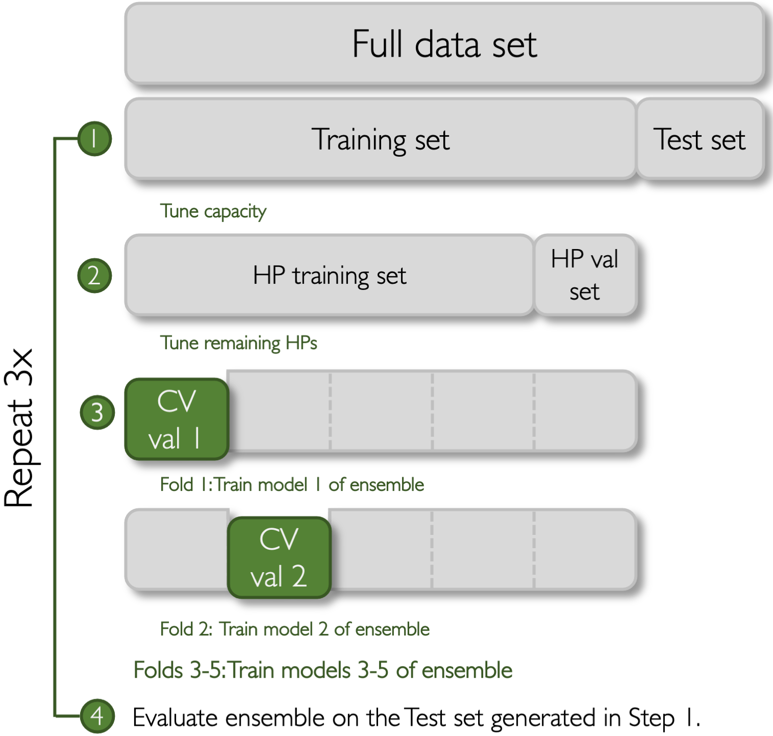
First, the entire data set for each property was randomly cut into 80% training, 20% test splits three times. All subsequent steps were performed for each training-test set pair. Using the NNDebugger package Gurnani 2021, the optimal capacity was found by attempting to overfit the entire training data set. The data set was considered overfit if the R2 value was greater than 0.97. If the data was not overfit, then the capacity corresponding to the highest R2 value was used. The capacity range considered was between two and fourteen. The training data set was then divided into an 80% hyperparameter (HP) training set and a 20% HP validation set. The remaining HPs (batch size, learning rate, dropout percentage) were optimized using the package scikit-optimize. The set of HPs corresponding to the lowest RMSE on the HP validation set was considered optimal.
Finally, the training data set was split into five folds using cross-validation (CV), producing one CV train data set and one CV validation data set per fold. For each fold, the model’s HPs were fixed as the optimal HPs and the model’s learnable parameters were fit to the CV train data set for 1000 epochs. At the end of 1000 epochs, the model parameters corresponding to the epoch with the lowest RMSE in the CV validation data set were chosen. After all five models were trained on their respective CV splits, the models were placed in an ensemble. The ensemble was used to make predictions of the test set, so far completely unseen by the ensemble during HP optimization or model training with CV.
All neural network architectures used dropout layers, fully connected layers, and Leaky ReLU activations (with a negative slope equal to ). All architectures were created using PyTorch and/or PyTorch Geometric. The weights of all models were optimized using the Adam optimizer and the mean squared error loss function. All weights were initialized according to a Xavier uniform distribution Glorot and Bengio 2010 with a gain of one. All biases were initialized using the default PyTorch setting.
S6 Extended Results
We computed both the root-mean-squared-error (RMSE) and Pearson correlation coefficient (R2) of each trained ensemble on unseen data for each property. The RMSE values are tabulated in the main body and the R2 values are tabulated in Table S1.
| Property | MT polyGNN | MT handcrafted PG | ST polyGNN | ST handcrafted PG |
| * | 0.106 0.245 | -0.177 0.205 | 0.002 0.209 | -0.367 0.678 |
| 0.840 0.019 | 0.824 0.023 | 0.757 0.032 | 0.777 0.018 | |
| 0.746 0.019 | 0.741 0.021 | 0.662 0.019 | 0.618 0.059 | |
| 0.913 0.004 | 0.901 0.004 | 0.885 0.011 | 0.892 0.004 | |
| * | 0.933 0.057 | 0.614 0.107 | 0.959 0.011 | 0.879 0.058 |
| * | 0.729 0.135 | 0.541 0.280 | 0.734 0.125 | 0.757 0.142 |
| * | 0.561 0.092 | 0.475 0.166 | 0.581 0.057 | 0.596 0.058 |
| * | 0.227 0.112 | 0.432 0.137 | 0.143 0.133 | 0.018 0.210 |
| * | 0.380 0.319 | 0.259 0.355 | 0.534 0.265 | 0.417 0.351 |
| 0.519 0.025 | 0.479 0.078 | 0.397 0.073 | 0.368 0.072 | |
| 0.894 0.022 | 0.777 0.034 | 0.900 0.014 | -4.126 4.386 | |
| * | 0.738 0.114 | 0.613 0.105 | 0.781 0.108 | 0.782 0.079 |
| * | 0.786 0.156 | 0.659 0.263 | -6553.467 11352.055 | 0.681 0.162 |
| * | 0.928 0.035 | 0.908 0.040 | 0.839 0.067 | 0.828 0.046 |
| 0.915 0.002 | 0.896 0.014 | 0.916 0.005 | 0.895 0.006 | |
| * | 0.557 0.358 | 0.652 0.088 | 0.354 0.404 | 0.683 0.197 |
| * | 0.842 0.102 | 0.896 0.088 | -0.494 0.851 | 0.224 0.503 |
| * | 0.750 0.252 | 0.807 0.255 | -12.141 21.000 | 0.166 0.302 |
| * | 0.819 0.144 | 0.704 0.199 | 0.203 0.125 | 0.168 0.116 |
| * | 0.861 0.071 | 0.888 0.062 | 0.346 0.178 | 0.441 0.232 |
| * | 0.797 0.088 | 0.720 0.149 | -0.553 2.096 | -1.899 3.879 |
| * | 0.519 0.219 | 0.670 0.078 | -0.913 1.112 | 0.013 0.531 |
| 0.860 0.042 | 0.813 0.060 | 0.815 0.066 | 0.742 0.084 | |
| * | 0.874 0.061 | 0.737 0.083 | 0.543 0.307 | 0.532 0.217 |
| 0.850 0.020 | 0.826 0.085 | 0.738 0.083 | 0.437 0.417 | |
| 0.501 0.107 | 0.587 0.094 | 0.428 0.176 | 0.480 0.073 | |
| 0.638 0.212 | 0.675 0.155 | 0.499 0.173 | 0.576 0.152 | |
| * | 0.770 0.074 | 0.235 0.180 | 0.536 0.156 | 0.686 0.045 |
| * | 0.969 0.002 | 0.978 0.007 | 0.877 0.037 | 0.891 0.023 |
| * | 0.983 0.002 | 0.988 0.002 | 0.914 0.018 | 0.857 0.041 |
| 0.980 0.006 | 0.981 0.006 | 0.866 0.027 | 0.779 0.174 | |
| 0.986 0.005 | 0.990 0.004 | 0.897 0.029 | 0.881 0.009 | |
| 0.985 0.003 | 0.988 0.003 | 0.833 0.070 | 0.844 0.034 | |
| 0.981 0.003 | 0.987 0.002 | 0.845 0.028 | -6.798 13.235 |
As discussed in the main body, we desire that the final output of each polyGNN model is approximately invariant to addition and subtraction. In other words, the variance in predictions between a set of equivalent repeat units should be low. As shown in Table S2, we find that our proposed data set augmentation does lead to a significant decrease in prediction variance a majority of the time.
| Property | |||
| 0.0237 | 0.0086 | 2.763 | |
| 0.0055 | 0.0014 | 3.840 | |
| 0.0144 | 0.0123 | 1.171 | |
| 0.0332 | 0.0177 | 1.874 | |
| 0.0414 | 0.0310 | 1.338 | |
| 0.0016 | 0.0021 | 0.7769 | |
| 0.0009 | 0.0020 | 0.4282 | |
| 0.0040 | 0.0062 | 0.6490 | |
| 0.0046 | 0.0011 | 4.318 | |
| 0.0088 | 0.0009 | 9.969 | |
| 0.0088 | 0.0018 | 4.807 | |
| 0.0049 | 0.0009 | 5.313 | |
| 0.0214 | 0.0145 | 1.480 | |
| 0.0186 | 0.0083 | 2.225 | |
| 0.0010 | 0.0010 | 0.9407 | |
| 0.0031 | 0.0018 | 1.765 | |
| 0.0014 | 0.0009 | 1.631 | |
| 0.0010 | 0.0005 | 2.156 | |
| 0.0010 | 0.0012 | 0.8613 | |
| 0.0019 | 0.0014 | 1.432 | |
| 0.0010 | 0.0026 | 0.3841 | |
| 0.0011 | 0.0012 | 0.8877 | |
| 0.0007 | 0.0011 | 0.6105 | |
| 0.0070 | 0.0079 | 0.8951 | |
| 0.0029 | 0.0027 | 1.089 | |
| 0.0167 | 0.0093 | 1.788 | |
| 0.0155 | 0.0088 | 1.764 | |
| 0.0165 | 0.0092 | 1.795 | |
| 0.0162 | 0.0066 | 2.454 | |
| 0.0178 | 0.0113 | 1.581 | |
| 0.0190 | 0.0117 | 1.630 | |
| 0.0036 | 0.0021 | 1.699 | |
| 0.0037 | 0.0022 | 1.690 | |
| 0.0096 | 0.0073 | 1.330 | |
| 0.0079 | 0.0014 | 5.774 | |
| 0.0123 | 0.0005 | 26.71 |
Table S2 contains the average variance of models trained with and without augmentation, and , respectively, on each of the 36 properties studied in this work. We define
where is a set of non-equivalent repeat units, is the variance function, is a machine learning model, and is a set of repeat units related to (a repeat unit in ) by addition or subtraction. In this work, is a set of 9 repeat units not seen by any model during training, and each is composed of and . For example, if is ( – C – ) then ( – C – ), ( – CC – ), ( – CCC – ), ( – CCCC – ), ( – CCCCC – )}.
Table S3 lists standard deviations of the data in our corpus, grouped by property.
| Property | |
| 0.0653 W/mK | |
| 109.3 K | |
| 114.7 K | |
| 109.0 K | |
| 0.470 | |
| 0.374 J/gK | |
| 13.10 | |
| 18.3 | |
| 0.0477 | |
| 23.7 | |
| 0.1991 g/cc | |
| 0.777 eV | |
| 1.101 eV | |
| 1.760 eV | |
| 1.561 eV | |
| 0.726 | |
| 1.388 | |
| 1.331 | |
| 1.276 | |
| 0.991 | |
| 1.039 | |
| 0.854 | |
| 0.359 | |
| 0.1713 | |
| 0.1142 | |
| 1.401 MPa | |
| 40.9 MPa | |
| 2.64 | |
| 0.806 Barrer | |
| 0.993 Barrer | |
| 1.207 Barrer | |
| 1.050 Barrer | |
| 0.950 Barrer | |
| 1.018 Barrer |