Improving Pulse-Compression Weather Radar via the Joint Design of Subpulses and Extended Mismatch Filter

In a weather radar system, sensitivity and resolution are the two important performance metrics. The sensitivity, referring to the minimum detectable reflectivity, is inversely proportional to the product of the pulse width and peak power [1]. Solid-state transmitters with high peak power are usually difficulty or expensive to obtain for most meteorological applications. Consequently, longer pulses must be transmitted to attain adequate sensitivity. However, the range resolution is proportional to the pulse width, and thereby longer pulses will results in the resolution degeneration. To tackle this dilemma, pulse compression can be the remedy for a low peak-power, long-duration coded pulse system to attain both the fine range resolution and improved sensitivity.

As a signal processing technique, pulse compression widens the bandwidth of the transmitted pulse by modulating it in either phase or frequency, and then the received echo is usually processed by a matched filter which compresses the long pulse to a short duration. The first attempt of implementing pulse compression on weather radar systems is back to 1970s [2], and some works investigated several technical and engineering aspects, see [3, 4, 5] and references therein. However, comparing to the wide applications in non-weather radars, its application on weather radar is relatively rare. The main obstacle lies in the range sidelobes introduced by the pulse compression, which is more notorious for weather radar since the targets of interest are usually extended volume scatters [6]. A large sidelobe will eventually cause inaccurate estimation of the reflectivity amplitude, which is a key index in meteorological applications. To tackle the issue of sidelobe, many works have been conducted recently [7, 8] although they were not primarily for the weather radar. In those works, the transmitted waveform is delicately designed to achieve a low peak or integrated sidelobe level.

For weather radar, benefiting from these developed techniques, the outlook towards using pulse compression could become promising after some appropriate adaptions. Motivated by this insight, in this paper, we investigate the joint design of transmit subpulses and mismatched filter for pulse compression weather radar. In general, we adopt the extended mismatched filter strategy with zero padding to improve sidelobes. Then we formulate the optimization problem and show the close relation among SINR, sidelobe and estimation error. To solve this nonconvex problem, we propose an efficient method based on the alternating direction method of multipliers (ADMM) [9]. The experiment results shows that the efficacy of the proposed pulse compression strategy and the enhanced performance.

Let $\bm{J}_{k}$ be a $N\times N$ shift matrix with the $(m,n)$-th entry being

Also, let $\bm{x}=[x_{1},x_{2},\ldots,x_{N}]^{T}\in{\mathbb{C}}^{N}$ be the transmitted fast-time radar code vector. Then, the received signal $\bm{y}\in\mathbb{C}^{N}$ after sampling from the range bin of interest is [10],

where $\alpha_{k},\forall k=-N+1,\ldots,N+1$ is a complex-valued scalar of atmospheric reflectivity corresponding to the $k$-th range bin illuminated by the radar pulse compression code, which is assumed to be independent and

and $\bm{\nu}\sim\mathcal{N}\left(\bm{0},\sigma_{\nu}^{2}\bm{I}\right)$ is the noise vector which is uncorrelated with the other signal-dependent terms.

One important step in weather radar is to estimate $\alpha_{0}$, which implies the hydrometer phenomena and is proportional to the reflectivity. In the conventional weather radars without pulse compression, the received signal in (2) does not contain the second term. Therefore, when using the pulse compression for a refined range resolution and lower peak power level, minimizing the introduced interference becomes critical.

By deploying mismatched-filter-like techniques, we can enlarge the filter length compared to the length of the subpulses after zero padding, which will spread the energy of the auto-correlation sidelobes into much larger coefficient space [6]. The subpulses after zero padding is defined by

and let $\widetilde{\bm{w}}\in\mathbb{C}^{\widetilde{N}}$ be the receive filter with $\widetilde{N}=2M+N$. The received signal after filtering can be obtained by

where $\widetilde{\bm{J}}_{k}$ is $\widetilde{N}\times\widetilde{N}$ shift matrix with the $(m,n)$-th entry being $1$ for $m-n=k$ and $0$ otherwise, and $\widetilde{\bm{\nu}}\sim\mathcal{N}\left(\bm{0},\sigma_{\widetilde{\nu}}^{2}\bm{I}\right)$.

The instrumental variable estimate of $\alpha_{0}$ is given by [10],

and its mean square error (MSE) is gievn by

where $\bm{R}=\sum_{\begin{subarray}{c}k=-\widetilde{N}+1,k\neq 0\end{subarray}}^{\widetilde{N}-1}\zeta_{k}\widetilde{\bm{J}}_{k}\widetilde{\bm{x}}\widetilde{\bm{x}}^{H}\widetilde{\bm{J}}_{k}^{H}+\sigma_{\widetilde{\nu}}^{2}\bm{I}$.

In addition, the received SINR for (5) can be expressed by

We can see that maximizing the SINR is equivalent to minimizing the above MSE. Further, $\widetilde{\bm{w}}^{H}\bm{R}\widetilde{\bm{w}}$ represents the sidelobe interference (ignoring the constant $\widetilde{\bm{w}}^{H}\widetilde{\bm{w}}$). Thus, maxmizing the SINR is essentially maximizing the signal-to-sidelobe ratio, which is desired in pulse compression design.

Based on the illustration, the problem is formulated as

Once the optimal $\widetilde{\bm{w}}$ and $\bm{x}$ are obtained, it is expected that the estimation of $\alpha_{0}$ will be enhanced by deploying the designed interpulses $\bm{x}$ and mismatched filter $\widetilde{\bm{w}}$.

In this section, we will focus on solving problem (9). The alternating optimization (AO) [11] will be deployed. For a fixed $\bm{x}_{t}$ at the $t$-th iteration of AO, the problem w.r.t $\widetilde{\bm{w}}$ is

with $\bm{R}_{t}=\sum_{\begin{subarray}{c}k=-\widetilde{N}+1,k\neq 0\end{subarray}}^{\widetilde{N}-1}\zeta_{k}\widetilde{\bm{J}}_{k}\widetilde{\bm{x}}_{t}\widetilde{\bm{x}}^{H}_{t}\widetilde{\bm{J}}_{k}^{H}+\sigma_{\widetilde{\nu}}^{2}\bm{I}$. It has a closed form solution $\widetilde{\bm{w}}=\bm{R}^{-1}_{t}\widetilde{\bm{x}}_{t}$.

For a fixed $\widetilde{\bm{w}}_{t+1}$, the problem w.r.t $\bm{x}$ can be written as

where $\bm{P}=\sum_{k=1}^{K}\zeta_{k}\bm{J}_{k}^{H}\bm{w}\bm{w}^{H}\bm{J}_{k}+\frac{\sigma^{2}}{N}\|\bm{w}\|^{2}$ and $\bm{Q}=\bm{w}\bm{w}^{H}$ with $\bm{w}=[\widetilde{\bm{w}}]_{M+1\mathrel{\mathop{\ordinarycolon}}M+N}$.

Through slack variables, problem (11) is equivalent to

Its Lagrangian function is

At the $\ell$-th iteration of ADMM, the update rules are

In the following, we focus on solving (14)-(a)(b)(c). For notation simplicity, we ignore the subscript $\ell$ and $\ell+1$.

For problem (14)(a), it becomes

where $\bm{a}=\frac{2}{\rho_{1}+\rho_{2}}\left[\rho_{1}\left(\bm{y}+\bm{u}\right)+\rho_{2}\left(\bm{z}+\bm{v}\right)\right]$. Since $\bm{x}^{H}\bm{x}=N$, the optimal solution to problem (15) is $\bm{x}=e^{j\arg\left(\bm{a}\right)}$.

For problem (14)(b), it can be further written as

where $\tilde{\bm{P}}=\frac{\bm{P}}{\bm{z}^{H}\bm{Q}\bm{z}}+\frac{\rho_{1}}{2}\bm{I}\succ\bm{0}$ and $\bm{b}=\rho_{1}\left(\bm{u}-\bm{x}\right)$. The closed form solution is $\bm{y}=-\frac{1}{2}\tilde{\bm{P}}^{-1}\bm{b}$.

For problem (14)(c), it becomes

with $\tilde{\bm{Q}}=\frac{\bm{Q}}{\bm{y}^{H}\bm{P}\bm{y}}\succeq\bm{0}$ with rank 1 and $\bm{c}=\rho_{2}\left(\bm{v}-\bm{x}\right)$. By letting $\tilde{\bm{Q}}=\bm{U}^{H}\bm{\Lambda}\bm{U}$ with $\bm{U}\bm{U}^{H}=\bm{U}^{H}\bm{U}=\bm{I}$, $\tilde{\bm{c}}=\bm{U}\bm{c}$, and $\tilde{\bm{z}}=\bm{U}\bm{z}$, problem (17) can be equivalently expressed as

Since $\text{rank}\left(\tilde{\bm{Q}}\right)=1$, $\bm{\Lambda}=\text{diag}\left(\left\{\lambda_{i}\right\}_{i=1}^{N}\right)$ with $\lambda_{1}=\frac{\|\bm{w}\|^{2}}{\bm{y}^{H}\bm{P}\bm{y}}$ and $\lambda_{2}=\cdots=\lambda_{N}=0$. Thus, the objective function of problem (17) can be expressed as

where $\tilde{z}_{i}$ is the $i$-th element of $\tilde{\bm{z}}$, $\hat{\bm{z}}=\left[\tilde{z}_{2},\ldots,\tilde{z}_{N}\right]^{T}$ and $\hat{\bm{c}}=\left[\tilde{c}_{2},\ldots,\tilde{c}_{N}\right]^{T}$.

Therefore, problem (18) can be decomposed into two independent problems. The first problem is as follows:

Since $\text{Re}\left(\tilde{c}_{1}^{*}\tilde{z}_{1}\right)\geq-\left|\tilde{c}_{1}\right|\left|\tilde{z}_{1}\right|$ with the equality achieved when $\arg\left(\tilde{z}_{1}\right)=\pi+\arg\left(\tilde{c}_{1}\right)$. Then, solving problem (20) is essentially solving

Let $t=\left|\tilde{z}_{1}\right|\geq 0$ and $g\left(t\right)=\frac{1}{\lambda_{1}t^{2}}+\frac{\rho_{2}}{2}t^{2}-\left|\tilde{c}_{1}\right|t$, then the first-order optimality condition is

After obtaining the positive root of the quartic polynomial, we can select the root with the largest value of $g\left(t\right)$. Hence, the optimal solution is $\tilde{z}_{1}=-te^{j\arg\left(\tilde{c}_{1}\right)}$.

The second problem is as follows:

which has a closed form solution $\hat{\bm{z}}=-\frac{1}{\rho_{2}}\hat{\bm{c}}$. Finally, the optimal solution of problem (18) is

The optimal solution to problem (17) is $\bm{z}=\bm{U}^{H}\tilde{\bm{z}}$.

In a summary, the derived algorithm will be double-loop, where the outer loop accounts for the AO between $\widetilde{\bm{w}}$ and $\widetilde{\bm{x}}$, and the inner loop accounts for the ADMM of $\widetilde{\bm{x}}$.

In this part, we study the performance of the optimized subpulse-filter pairs in weather observation. We conduct our simulation using a radar simulator [12], which generates time series data for the NEXRAD WSR88D radar specifications¹¹ 1 The polarimetric weather radar NEXRAD WSR88D operates in $2.8$ GHz and has a maximum unambiguous range of $100$ km with $250$m resolution. [13]. Following the same procedure as suggested by [6], we convolve the simulated weather echoes with the transmit subpluses, which imposes the effect of pulse compression waveform. Next, we convolve the obtained uncompressed samples with the filter coefficients. Hence, we assess the utility of the optimized subpluse-filter pair based on Level-II information from NEXRAD WSR88D.

Fig. 1 shows the convergence of the proposed algorithm, from which we observe that the objective value decreases monotonically as the iteration goes.

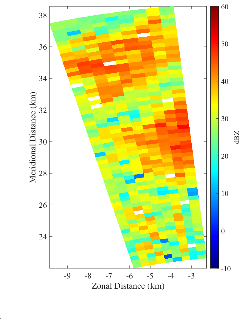
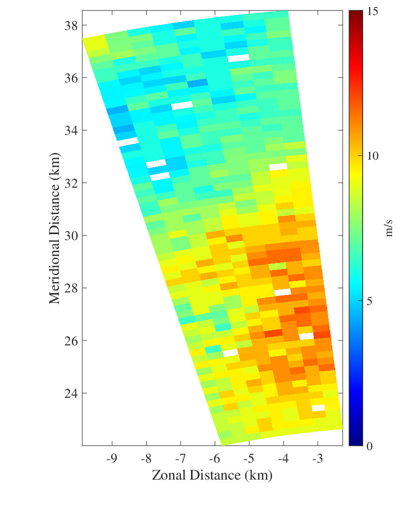
In Figure 2, we set $N=\widetilde{N}=100$ and evaluate the horizontal reflectivity²² 2 The reflectivity $Z$ (in units of $mm^{6}/m^{3}$) commonly span many orders of magnitude, and hence a logarithmic scale $\text{dB}Z=10\log_{10}Z$ is used. and radial velocity³³ 3 Radial velocity refers to the first moment of the power-normalized spectra, which reflects the air motion toward or away from the radar. for real data and the simulated time series utilizing the optimized subpulse-filter pairs. It can be observed that the simulated result mimic the behaviour of the real data, which indicates the efficacy of utilizing the designed pulse compression.

Figure 3 indicates the difference in the phase delay ($\phi_{DP}$) of the returned signal from the benchmark and simulated data by using the proposed method. The values of $\phi_{DP}$ provides information on the nature of the scatterers that are being sampled. By these comparisons, it can be observed that the radar moment estimation is consistent to the NEXRAD specifications, which indicates high quality of the optimized subpulse-filter pairs in weather radar applications.

We propose an optimization-based method for implementing a delicate pulse compression on weather radar. Through the proposed method, the transmitted subpulse codes and the extended filter are jointly designed, which guarantees that the pulse compression will possess a low sidelobe level and further a better estimation of the meteorological reflectivity. The experiments result demonstrates the efficacy of the proposed approach and the improvement brought by this delicately designed pulse compression technique.

References

- [1] V. N. Bringi and V Chandrasekar, Polarimetric Doppler Weather Radar: Principles and Applications, Cambridge University Press, 2001.
- [2] R. W. Fetter, “Radar weather performance enhanced by pulse compression,” in Proceedings of 14th AMS Conf. Radar Meteorol, 1970, pp. 413–418.
- [3] A. S. Mudukutore, V Chandrasekar, and R. J. Keeler, “Pulse compression for weather radars,” IEEE Transactions on geoscience and remote sensing, vol. 36, no. 1, pp. 125–142, 1998.
- [4] J. George, N. Bharadwaj, and V Chandrasekar, “Considerations in pulse compression design for weather radars,” in IGARSS 2008-2008 IEEE International Geoscience and Remote Sensing Symposium. IEEE, 2008, vol. 5, pp. V–109.
- [5] R. M. Beauchamp, S. Tanelli, E. Peral, and V Chandrasekar, “Pulse compression waveform and filter optimization for spaceborne cloud and precipitation radar,” IEEE Transactions on Geoscience and Remote Sensing, vol. 55, no. 2, pp. 915–931, 2016.
- [6] M. Kumar and V Chandrasekar, “Intrapulse polyphase coding system for second trip suppression in a weather radar,” IEEE Transactions on Geoscience and Remote Sensing, vol. 58, no. 6, pp. 3841–3853, 2020.
- [7] J. Song, P. Babu, and D. P. Palomar, “Optimization methods for designing sequences with low autocorrelation sidelobes,” IEEE Transactions on Signal Processing, vol. 63, no. 15, pp. 3998–4009, 2015.
- [8] M. A. Kerahroodi, A. Aubry, A. De Maio, M. M. Naghsh, and M. Modarres-Hashemi, “A coordinate-descent framework to design low psl/isl sequences,” IEEE Transactions on Signal Processing, vol. 65, no. 22, pp. 5942–5956, 2017.
- [9] S. Boyd, N. Parikh, and E. Chu, Distributed optimization and statistical learning via the alternating direction method of multipliers, Now Publishers Inc, 2011.
- [10] P. Stoica, J. Li, and M. Xue, “On binary probing signals and instrumental variables receivers for radar,” IEEE Transactions on Information Theory, vol. 54, no. 8, pp. 3820–3825, 2008.
- [11] U. Niesen, D. Shah, and G. W. Wornell, “Adaptive alternating minimization algorithms,” IEEE Transactions on Information Theory, vol. 55, no. 3, pp. 1423–1429, 2009.
- [12] “Simulating a polarimetric radar return for weather observation,” https://nl.mathworks.com/help/radar/ug/simulating-a-polarimetric-radar-return-for-weather-observation.html, Accessed: 2021-12-16.
- [13] “Nexrad technical information,” https://www.roc.noaa.gov/WSR88D/Engineering/NEXRADTechInfo.aspx, Accessed: 2021-12-16.