Exploiting Transformer in Sparse Reward Reinforcement Learning for Interpretable Temporal Logic Motion Planning Thanks: Manuscript received: March 3, 2023; Revised: May 8, 2023; Accepted: June 22, 2023. This paper was recommended for publication by Editor Jens Kober upon evaluation of the Associate Editor and Reviewers’ comments. This work was supported in part by the National Natural Science Foundation of China under Grant 62173314 and U2013601. (Corresponding Author: Zhen Kan)Thanks: H. Zhang, H. Wang, and Z. Kan are with the Department of Automation at the University of Science and Technology of China, Hefei, Anhui, China, 230026.Thanks: Digital Object Identifier (DOI): see top of this page.
Abstract
Automaton based approaches have enabled robots to perform various complex tasks. However, most existing automaton based algorithms highly rely on the manually customized representation of states for the considered task, limiting its applicability in deep reinforcement learning algorithms. To address this issue, by incorporating Transformer into reinforcement learning, we develop a Double-Transformer-guided Temporal Logic framework (T2TL) that exploits the structural feature of Transformer twice, i.e., first encoding the LTL instruction via the Transformer module for efficient understanding of task instructions during the training and then encoding the context variable via the Transformer again for improved task performance. Particularly, the LTL instruction is specified by co-safe LTL. As a semantics-preserving rewriting operation, LTL progression is exploited to decompose the complex task into learnable sub-goals, which not only converts non-Markovian reward decision processes to Markovian ones, but also improves the sampling efficiency by simultaneous learning of multiple sub-tasks. An environment-agnostic LTL pre-training scheme is further incorporated to facilitate the learning of the Transformer module resulting in an improved representation of LTL. The simulation results demonstrate the effectiveness of the T2TL framework.
I Introduction
One of the ultimate goals in robotic learning is to let the robot infer the key to the task completion. To enable such human-level intelligence, the capability of comprehending the semantics of instructions and evolving continuously via interactions with the environment is crucial. Among numerous learning algorithms, reinforcement learning (RL) is a sequential decision-making process that models dynamics of the interaction as a Markov decision process (MDP) and focuses on learning the optimal policy through exploration and exploitation [1]. Although RL based methods have enabled the robot to accomplish tasks from simple to complex ones, an important yet challenging topic is how the robot can enhance their understanding of instructions to improve task completion. In particular, there are three main challenges: 1) unlike existing works with explicit task instructions and motion constraints, how can the robot comprehend the nature of instructions by its own to improve the task completion? 2) Since many practical tasks require the robot to perform a series of logically organized sub-tasks (e.g., cleaning rooms, organizing books and washing clothes while avoiding collisions), resulting in a non-Markovian reward decision process (NMRDP), how can the NMRDP be properly handled? 3) When solving the complex task in a sparse reward environment, how can the robot facilitate learning by leveraging the potential of its representation module?
Transformer was originally presented in [2] for natural language processing and recently achieves remarkable success in many fields. In [3], a Vision Transformer (ViT) framework is developed, which proposes patch embedding for image preprocessing and performs better than state-of-the-art CNNs. The work of [4] presents an effective combination of RL and Transformer, which casts the traditional RL problem as a conditional sequence modeling by leveraging the causally masked Transformer. The structured features of Transformer are further incorporated in [5] to improve robotic manipulation by capturing the spatio-temporal relationship between the dual-arm movements. Despite recent progress, most of the existing methods with Transformer mainly focus on natural language processing or computer vision, lacking the guidance to drive robots towards task completion. It is unclear how conventional Transformer can be combined with RL to guide the agent to understand complex motion planning tasks that consist of a series of sub-goals that need to be completed logically.
Due to the rich expressivity and capability, linear temporal logic (LTL) is capable of describing a wide range of complex tasks composed of logically organized sub-tasks [6]. By converting the LTL specification into an automaton, learning algorithms are often exploited to facilitate the motion planning of robotic systems. For instance, modular deep reinforcement learning is incorporated with a limit deterministic generalized Büchi automaton (LDGBA) to enable continuous motion planning of an autonomous dynamical system [7]. Learning-based probabilistic motion planning subject to the deterministic Rabin automaton (DRA) guideline in the presence of environment and motion uncertainties is investigated in [8]. Truncated LTL is leveraged to facilitate the reward design in [9], which can be converted into a finite-state predicate automaton (FSPA) to improve the performance of reinforcement learning in robotic planning. Similar to the automaton, reward machine (RM) is proposed to offer dense rewards feedback in [10], which can be translated from a variety of temporal logic specifications to improve the sample efficiency of reinforcement learning methods. However, most of these aforementioned methods highly rely on the representation of system states in the form of either automaton or RM, which not only grows exponentially with respect to the task complexity, but also are not effective for deep learning (i.e., the customized automaton states with sorted index or manually one-hot encoding in RM generally cannot facilitate the gradient propagation of neural networks). When considering representing the LTL as a neural network, the work of [11] exploits a compositional recurrent neural network (RNN) as an encoder to train the learning agent to understand LTL semantics. However, RNN generally suffers from high computational cost due to its inherently sequential nature precluding parallelization. In [12], the compositional syntax and the semantics of LTL are exploited by the relational graph convolutional network (R-GCN) to enable the generalization to new tasks. However, it cannot offer interpretable guidance to the agent due to irregularity of the R-GCN architecture [13].
To bridge the gap, we consider using Transformer to encode the LTL specifications to provide a more appropriate representation to improve the performance, and offer reasonable interpretability for task completion.
The main contributions of this work are summarized as follows:
1. To our best knowledge, this is the first work that encodes LTL instructions by Transformer to accomplish a complex task with Reinforcement Learning in a sparse reward environment, whose representation not only yields better policy performance than traditional one-hot encoding or sorted index representations, but also further provides reasonable interpretability for the agent’s motion planning.
2. We develop a Double-Transformer-guided Temporal Logic framework (T2TL) that exploits the structural feature of Transformer twice, which first encodes the LTL instruction via the Transformer module for efficient understanding of task instructions during the training and then encodes the context variable via the Transformer again to capture the intrinsic relativity of sub-tasks. We evaluate our method on two continuous control tasks. The performance and statistical analysis demonstrate the effectiveness of our approach.
3. LTL progression, as a semantics-preserving rewriting operation, is exploited to decompose the complex instruction into learnable sub-goals, which not only converts non-Markovian reward decision processes to Markovian ones, but also improves the sampling efficiency by simultaneous learning of multiple sub-tasks. Inspired by [12], an environment-agnostic LTL pre-training scheme is further incorporated to facilitate the learning of Transformer.
II Preliminaries
II-A Co-Safe Linear Temporal Logic
Co-safe LTL (sc-LTL) is a subclass of LTL that can be satisfied by finite-horizon state trajectories [14]. Since sc-LTL is suitable to describe robotic instructions (e.g., trigger the alarm, find the extinguisher, and then put out the fire), this work focuses on sc-LTL. An sc-LTL formula is built on a set of atomic propositions that can be true or false, standard Boolean operators such as (conjunction), (disjunction), and (negation), temporal operators such as (next), (eventually), and (until). The semantics of an sc-LTL formula are interpreted over a word , which is a finite sequence with , , where represents the power set of . Denote by if the sc-LTL formula holds from position of . More detailed explanations and examples can be found in [6].
II-B Labeled MDP and Reinforcement Learning
When performing the sc-LTL task , the interaction between the robot and the environment can be modeled by a labeled MDP , where is the state space, is a set of terminal states, is the action space, is the transition probability from to under action , is a set of atomic propositions indicating the properties associated with the states, is the labeling function, is the reward function, is the discount factor, and is the initial state distribution. The labeling function can be seen as a set of event detectors that trigger when presents in the environment, allowing the robot to determine whether or not an LTL specification is satisfied. It is assumed that the transition probability is unknown a priori, and the agent can only perceive its state and the corresponding label.
For any task , the robot interacts with the environment following the policy over . Specifically, the robot starts from an initial state sampled from in each episode, and transits from the current state to the next state following under the control action generated by the policy . The robot then receives a reward by . The Q-value is and the optimal Q-value is . The optimal policy can be derived from the optimal Q-value.
When applying to a large or continuous state space, the Q-value function is often parameterized with the weights function like in the Deep Q-Networks (DQN) [15]. And in the continuous action case, the parameterized policy model is often applied to the uncountable infinite problem like with weights as in Proximal Policy Optimization (PPO) [16]. The typical reward function is often Markovian, which means that the reward acquired at is only based on the transition from to . In practice, however, the robot is generally rewarded when the corresponding word satisfies the LTL task , denoted as , and the episode terminates when is satisfied or falsified. Since the word is formed from the state trajectory through the labeling function , in this work we will consider the non-Markovian reward function
| (1) |
where . In the sequel, we will discuss how to deal with the challenge of NMRDP. Given a task , the goal of the agent is to learn an optimal policy that maximizes the expected discounted return starting from any state at time step .
III Problem Formulation
To elaborate the proposed interpretable temporal logic guided reinforcement learning algorithm, the following example will be used as a running example throughout the work.
Example 1.
Consider a modified safety-gym environment [17], in which the robot is required to sequentially visit a set of locations while avoiding collisions. The set of propositions is {}. Using above propositions in , an example sc-LTL formula is where , which requires the robot to sequentially visit the black zone and the white zone while avoiding colliding with red zones and yellow zones.
In this work, we are interested in encoding the task conditional states by the Transformer. By representing via Transformer we hope to take advantage of its flexibility in encoding states and provide interpretable analysis of the robot’s motion planning. Compared with automaton and RM-based state representations, when using Transformer to encode the states, the gradually updated state representation can facilitate the agent’s comprehension of the sub-goal at hand as the agent interacts with the environment, resulting in a mutual improvement, in which the Transformer guides the robot’s motion and the selected actions improve the Transformer for better instructions.
Specifically, suppose the representation of an LTL task can be approximated by the Transformer parameterized with weights , where is updated by the back-propagation of the RL controller. The goal of an interpretable LTL guided RL in this work is to find the appropriate Transformer weights over the LTL instruction, such that an effective representation can lead to fast learning for logical motion planning. To this end, the problem can be formally presented as follows.
Problem 1.
Given a MDP corresponding to task with the reward function to be designed, the goal of this work is to design an optimal representation with , so that the return under the policy can be maximized.
IV Algorithm Design
To address Problem 1, this section presents a novel framework, namely Double-Transformer-guided Temporal Logic framework (T2TL), that offers interpretable LTL instruction using Transformer to guide the robot motion planning and uses Transformer again to encode context variables to further facilitate the robot learning. Section IV-A presents how LTL progression can be leveraged to convert NMRDP to MDP. Section IV-B explains how the Transformer is exploited to encode the LTL specification. Section IV-C explains in detail how Transformer can facilitate the agent’s understanding of complex tasks using simultaneous learning. Section IV-D shows how the context variable improves the agent performance and how the pre-training scheme can be further incorporated to expedite the convergence.
IV-A LTL Progression and TL-MDP
One of the major challenges in solving Problem 1 is that the reward function used in the Q-value function depends on the history of the states and thus is non-Markovian. In this work, the LTL progression from [18] is applied to solve the non-Markovian issue. Let denote the propositions needed to progress the current LTL specification. The LTL progression is defined formally as follows.
Definition 1.
Give an LTL formula and a word , the LTL progression at step , is defined as follows:
The operator in Def. 1 takes an LTL formula and the current label as input at each step, and outputs a formula to track which parts of the original instructions remain to be addressed.
Theorem 1.
[18] Given any LTL formula and the corresponding word , .
There are many advantages of using the LTL progression. First, since the operator can preserve LTL semantics, applying iteratively after each step will result in gradually diminishing LTL instructions, which indicates the progress towards task completion. Therefore, the reward function can be designed by leveraging it to make the agent focus on the current progressed task rather than the original one all the time. Another benefit of utilizing iteratively is that the complex task may be divided into a series of learnable sub-tasks that can be viewed as simultaneous sub-goals to improve the sampling efficiency. In the following context, we represent by the extended training set for which and its progressed sub-tasks are included.
Based on the LTL progression in Def. 1 and the LTL instruction , an augmented MDP, namely the task-driven labeled MDP (TL–MDP), is developed as follows.
Definition 2.
corresponding to an LTL task , the TL–MDP is constructed by augmenting to with indicating the number of tasks in , where , , if and otherwise, and is the reward function associated with the task to overcome the non-Markovian reward issue which can be written as
| (2) |
Thus, by defining the TL-MDP, the non-Markovian reward function can be Markovian. With LTL progression, the policy that solves the LTL over the TL-MDP can achieve the same expected discounted return as the policy in the environment [12].
IV-B Represent LTL via Transformer
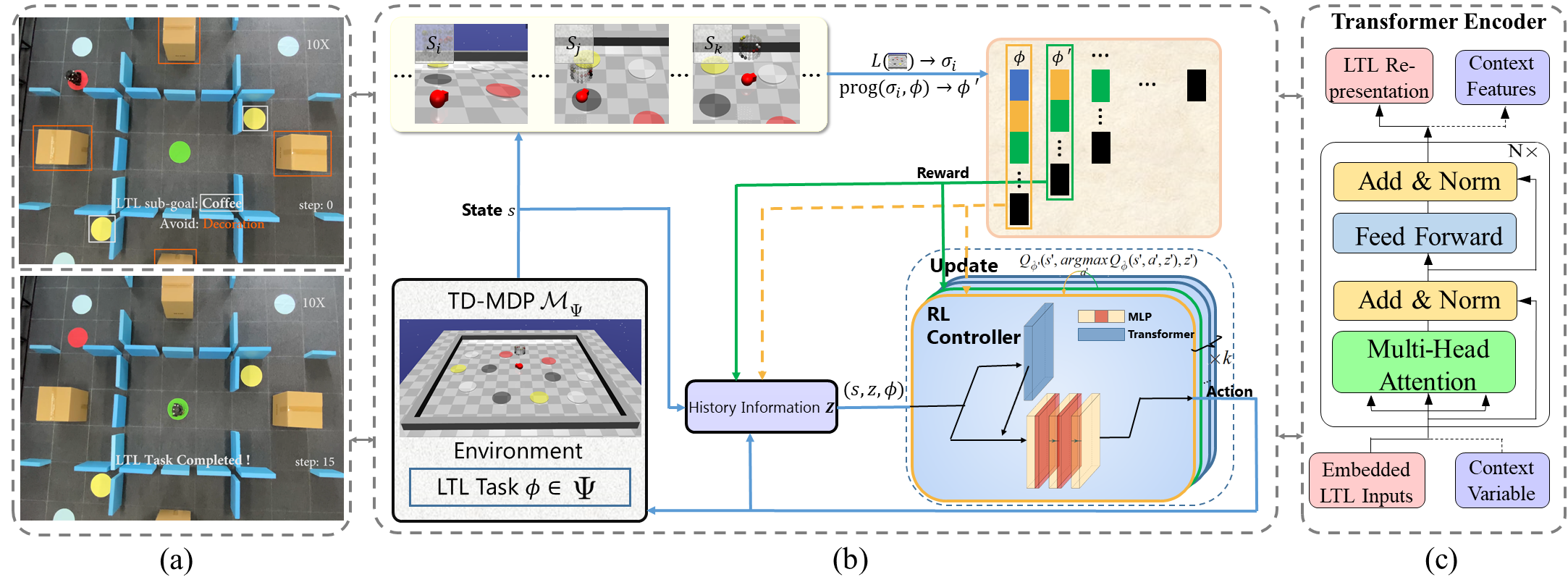
Another challenge in solving Problem 1 is to design an appropriate parameterized encoder for the LTL specification for improved performance without shaping the reward function [19, 20] or using special exploration strategies [21] in a sparse reward environment. To address this challenge, inspired by the interpretable representation architecture and encoding capability for the nature language, the Transformer from [2] is exploited to represent the LTL instruction in this work. An overview of the architecture is depicted in Fig. 2(b).
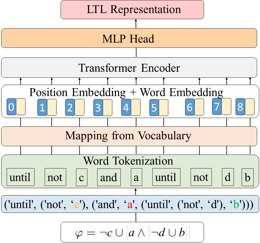
Given an input generated by the LTL task where represents the operator or proposition, will be preprocessed by the word embedding as where is the batch size, is the length of input , and is the model dimension of the Transformer. is then added with the frequency-based positional embedding to make use of the order of the sequence. For instance, a task can be encoded as shown in Fig. 1.
The encoder is constructed by stacking identical transformer layers and each transformer layer is built with a self-attention sub-layer and a position-wise fully connected feed-forward (MLP) sub-layer. Layer norm (LN) is applied before every sub-layer and residual connections are applied after every block. In the structure of the Transformer, the multi-head self-attention (MSA) method plays an important role in establishing the intrinsic connections between words. Specifically, given the query , key , and value derived from the LTL input , the similarity of words can be calculated by the dot-product attention as
where is the scaling factor. The global computation procedure of the encoder layers is represented as follows:
where represents the output of the last layer from the Transformer encoder, which can be manually customized to an appropriate dimension according to the need of tasks.
Motivated by [22] and [23], the weights or heads of self-attention in Transformer can offer reasonable interpretability for the agent’s motion planning in RL. Specifically, given the weights , the interpretability can be indicated by showing on which proposition (i.e., the sub-task in LTL to be solved) the head’s weights are more focused according to where and is the number of heads in Transformer. Note that, since this work involves Transformer inputs that do not consider a co-reference candidate, (e.g., the gender bias), all heads are equally important and do not have pre-set emphasis tokens to generate top heads like [22].
IV-C T1TL and Simultaneous Learning
As shown in Table I, traditional product-MDP algorithms usually represent the states of automaton or RM with one-hot encoding or sorted index, whose representation needs to be customized manually and the dimensions are dependent on the complexity of the LTL task. Unlike these works, we encode the LTL specification as normalized vectors using Transformer, which is not only appropriate for the forward propagation of the neural network, but also can be continuously updated as Transformer evolves. In addition, its dimension can be customized with appropriate designs of Transformer, leading to improved agent’s performance. Compared with automaton-based methods, the product-MDP based Transformer can be constructed on-the-fly without concern of exponential explosion of algorithm complexity with LTL tasks.
| Automaton or RM | Transformer | |
| Dimension | fixed (limited by LTL task complexity) | flexible |
| Representation | customize manually | update via Transformer |
| Construction | in advance (in most cases) | on-the-fly |
| Interpretability | indirect (interpreted by some | direct (interpreted by weights |
| module in other models) [24, 25, 26] | or heads in self-attention) | |
| Effect | limited by dimension | better with appropriate dimensions |
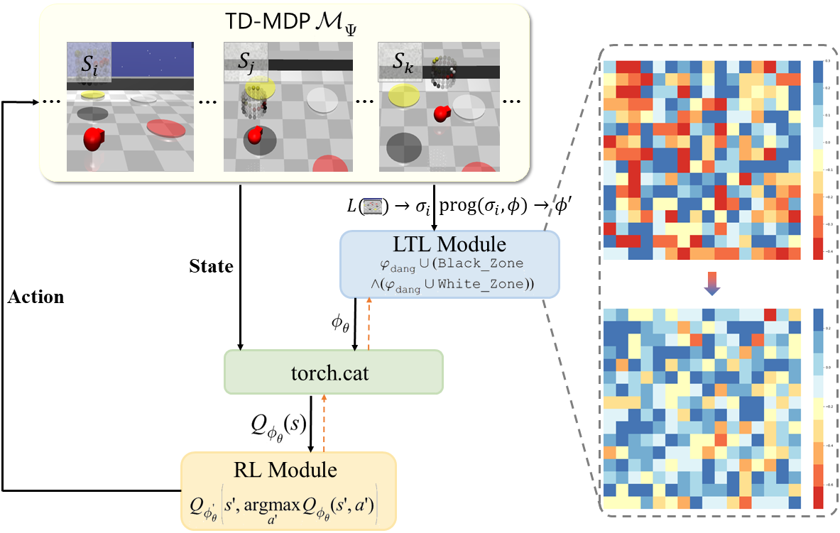
The interpretable LTL representation encoded via the Transformer is illustrated in Fig. 3. Initially, the weights of Transformer are set randomly. As the agent interacts with the environment, the RL module is updated when a proposition is encountered by the agent, which leads to an indirect update of the Transformer module, i.e., the agent has new knowledge of the pros and cons about the currently encountered proposition for completing the task. Thus, as the RL module converges, the Transformer module achieves a better representation of the LTL instruction. Meanwhile, as the representation of LTL becomes more effective, the convergence of the RL policy is further improved. Let and be the Q-value function of task and , respectively. Thus in the conventional RL algorithm, such as DQN, the update for driven by the Transformer can be written as
However, conventional off-policy DRL algorithm usually performs a random exploration in the early stage. If an action effective for other tasks is performed rather than the current task, such an action is often ignored and will not be utilized to update the Q-value for associated tasks, resulting in low sampling efficiency and delayed convergence to the optimal policy. Note that the on-policy DRL algorithms, such as PPO, usually train the agent with parallel environments to improve sampling efficiency by reducing the correlation of transition data. However, this trick usually can’t be applied to off-policy DRL algorithm due to the experience replay buffer.
Compared with vanilla DQN, the idea of simultaneous learning is to extract sub-tasks from via LTL progression as described in Sec. IV-A, augment the original MDP with the LTL representation encoded by Transformer module, and use Q-learning to simultaneously learn these sub-tasks.
Particularly, the simultaneous learning begins with extracting sub-tasks from by LTL progression to generate an extended training set . All tasks are associated with a Q-value function where the LTL instruction is encoded by the Transformer module, and a series of episodes over the tasks in is performed using the off-policy learning method. For each , the robot updates the Q-value functions as if it is currently trying to solve . Specially, given the current state , the formula will be the progressed LTL task if . The robot selects an action following a behavior policy (e.g., the -greedy one) based on the Q-value and then transits to the next state with rewards received from (2). Let and be the Q-value function of task and , respectively. Thus under the simultaneous learning, is updated following a modified double DQN as
| (3) |
By this way, the Q-value of will be propagated backwards from its sub-tasks and the weights of Transformer will also be updated over the state representation. Thus by developing TL-MDP , it will not only convert the non-Markovian reward processes to Markovian ones, but also provide simultaneous update for sub-task’s Q-value. Such a method enables the update of the current and its sub-task , resulting in an effective representation of LTL for improved convergence.
IV-D T2TL and Pre-training Scheme
Since LTL progression decomposes the original LTL specification into sub-goals that can be learned simultaneously in Sec. IV-C, the context variable that captures the connections of simultaneous sub-goals is further incorporated using Transformer. The context variable in meta reinforcement learning (meta-RL) [27] is used to capture the intrinsic relativity of multiple tasks. In [28], an off-policy meta-RL with the probabilistic context variable is developed, which enhances adaptation efficiency using posterior sampling during training. The work of [29] adopts the deterministic context variable to further improve the learning performance.
Considering the effectiveness and compatibility, the deterministic context variable is applied. Specially, a deterministic context variable acts as a fixed length window and extracts the knowledge of history observations, actions and rewards in a certain range when the agent explores the environment. Different from [29] that uses RNN, Transformer is leveraged to encode the context variable in this work, which facilitates the convergence of the LTL representation. Thus the Q-value function is then conditioned on the context as , where is a deterministic context variable, and (3) can be augmented as
| (4) |
By this way, the robot is able to comprehend the LTL task by considering the context information and expedite the learning in a sparse reward environment.
Inspired by the competitive performance on downstream tasks when using the pre-training method in [12], an environment-agnostic module is further incorporated as the pre-training scheme in this work. First, a single-state MDP is built, where , , , , and . Then the single-state MDP can be augmented to TL-MDP with the LTL instruction . Second, the agent tries to complete the LTL task in each episode until the Transformer module converges. At the end of the pre-training, the learned Transformer weights are then transferred to the downstream MDP as the initial LTL Module (e.g., the TL-MDP in the revised safety-gym). Note that the design of is to learn a policy that satisfies the LTL task as quickly as possible by choosing one proposition to be true at each time step. With the pre-training scheme, the LTL presentation from can help the agent infer which part of the information should be emphasized to increase the probability of achieving sub-goals. The overall method is illustrated in Fig. 2(a) and the pseudo-code is outlined in Alg. 1.
V CASE STUDIES
In this section, the developed T2TL framework is evaluated against the state-of-the-art algorithms in simulation11 1 Our codes are avaliable at https://github.com/Charlie0257/T2TL. Specifically, we consider the following aspects. 1) Performance: how well does our approach outperform the state-of-the-art algorithms in two continuous environments? 2) Representation: What is the role of the representation dimensions for LTL specifications? 3) Interpretability: How well can the agent understand LTL specifications via Transformer?
To show the effectiveness of the T2TL framework, denoted by , it is empirically compared with four baselines. The first baseline is DFA from [30] which is used to construct the product MDP for the LTL task over a finite horizon. The second baseline is RM from [10] which has automaton-based representations that exploit the reward function’s internal structure to learn optimal policies. The third baseline is , which uses a pre-training scheme from [12] and exploits the compositional syntax and semantics of LTL by GNN to solve complex multiple tasks. Note that the simultaneous learning is incorporated in for fair comparisons with our method. The fourth baseline is , which exploits Transformer instead of GNN to encode LTL instructions with a pre-training scheme. The fifth baseline is , which is based on DFA and uses Transformer to encode the context variable to capture the intrinsic connection between sub-tasks.
To evaluate the performance in a sparse reward environment, our framework is verified in two different continuous cases. The RL algorithms applied to two cases are double DQN [31] and PPO [16] respectively to show the generality of our method over the on-policy and off-policy RL.

(1) Case 1: WaterWorld. We first evaluate the developed T2TL framework in a dynamic continuous world [10]. As shown in Fig. 4(a), each ball moves at a fixed velocity in a certain direction and bounces when it hits a wall. The agent represented by the white ball can increase its speed in any of the four cardinal directions. The set of propositions in this environment is composed of balls of different colors. In this scenario, we consider an sc-LTL task , where , which requires the agent to encounter the ball with , , , and in order while avoiding , and balls.
Fig. 4(b) shows the performances of all baselines against ours over the task with 12 random seeds in the WaterWorld environment. Clearly, the method of simultaneous learning shows improved convergence than . By encoding the LTL representation using Transformer, outperforms RM and . By incorporating context variable, shows better performance at the end.

(2) Case 2: ZoneEnv. We further evaluate our framework in a modified Safety-gym [17] environment as shown in Fig. 5(a). Consider a sequential task requiring the robot to visit the red zone, black zone, and yellow zone in order, which can be written as Fig. 5(b) shows the performance of and , which outperform clearly, reflecting the effect of the LTL representation encoded by neural networks. shows a competitive performance compared with and .
| Task Level | T1TL_pre | GNN_pre | RM |
|---|---|---|---|
| 5 sub-goals with 1 obstacle | 236.50(4.49) | 253.26(6.57) | 259.13(3.06) |
| 5 sub-goals with 2 obstacles | 286.77(5.21) | 310.50(6.24) | 322.56(13.47) |
| 5 sub-goals with 3 obstacles | 421.31(8.32) | 468.73(9.02) | 489.07(14.17) |
| Task Level | T1TL_pre | GNN_pre | RM |
|---|---|---|---|
| 4 sub-goals with 1 obstacle | 189.46(1.98) | 191.71(3.25) | 207.21(8.03) |
| 5 sub-goals with 1 obstacle | 236.50(4.49) | 253.26(6.57) | 259.13(3.06) |
| 6 sub-goals with 1 obstacle | 609.82(15.73) | 628.29(21.92) | 659.32(6.39) |
| Task Level: | T1TL_pre | GNN_pre | RM |
|---|---|---|---|
| 5 sub-goals with 2 obstacles (size: 1x) | 286.77(5.21) | 310.50(6.24) | 322.56(9.47) |
| 5 sub-goals with 2 obstacles (size: 1.5x) | 291.94(2.18) | 305.85(8.04) | 338.57(10.24) |
| 5 sub-goals with 2 obstacles (size: 2.5x) | 269.88(5.00) | 276.34(7.48) | 300.78(12.20) |
(3) Statistical Analysis for Representations. To further show the benefits of Transformer-encoded representation, we compare the average steps used by different representation methods when completing the task of different complexities in the WaterWorld environment. As shown in Table II, as the number of obstacles increases, the Transformer-encoded representation uses fewer steps than the baselines. In Table III, the representation encoded by Transformer still shows better performance than the baselines. Table IV shows more stable performance can be achieved using Transformer when the size of the obstacle becomes larger.
| WaterWorld | RM | ||||
|---|---|---|---|---|---|
| 1.96(0.08) | 2.60(0.05) | 1.95(0.03) | 2.20(0.20) | 2.02(0.52) |
| ZoneEnv | |||||
|---|---|---|---|---|---|
| 12.21(7.16) | 11.09(7.46) | 9.60(5.85) | 3.12(2.80) | 6.61(5.63) |
(4) Statistical Analysis for Performance in Unit Time. To further evaluate the performance of different methods per unit of time, we define the unit performance as where is the number of total episodes or total steps, is the reward in one episode or fixed steps, is the elapsed time in one episode or fixed steps, and is the pre-training time. As shown in Table V, spends more time updating the double Transformer framework, while yields better performance compared to other algorithms. As shown in Table VI, can improve the sampling efficiency and shows better performance in more challenging environments.

(5) Dimension Comparison. To emphasize the influence of the representation dimension of the LTL instruction on agent performance in a high-dimensional state space or complex environment, Fig. 6 shows the results between and traditional methods by one-hot encoding with different dimensions in the WaterWorld and ZoneEnv environment. It is clear in Fig. 6(a) that an appropriate increase for the representational dimension of the LTL instruction is beneficial in providing agents with more comprehensive information. In Fig. 6(b), an appropriate representational dimension further improves the performance of DFA, and the agent achieves good performance when the dimension is 16 in .
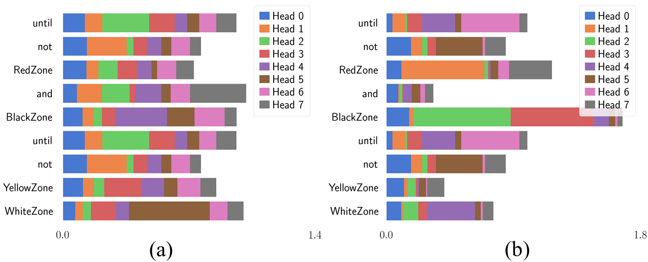
(6) Interpretability via Attention. To further visualize how well the agent understand the LTL task when the Transformer module converges, Fig. 7 shows a view from heads in attention to interpret which tokens the agent would be more interested in. In Fig. 7, different color bars represent different heads in the layers of attention and its length indicates the weights of the head on this token. As shown in Fig. 7(a), all heads are distributed with almost identical weights on different tokens at the beginning of the training, reflecting the fact that the agent doesn’t have a clear concept of LTL instruction at the moment. However, when the Transformer module converges, more weights focus on the token as shown in Fig. 7(b), which implies the agent having a greater probability of going directly to the proposition .
VI CONCLUSIONS
In this work, we present a T2TL framework that incorporates Transformer to represent the LTL formula for improved performance and interpretability. Future work will consider extensions to multi-task learning.
References
- [1] R. S. Sutton and A. G. Barto, Reinforcement learning: An introduction. MIT press, 2018.
- [2] A. Vaswani, N. Shazeer, N. Parmar, J. Uszkoreit, L. Jones, A. N. Gomez, Ł. Kaiser, and I. Polosukhin, “Attention is all you need,” Adv. neural inf. process. syst, vol. 30, 2017.
- [3] A. Dosovitskiy, L. Beyer, A. Kolesnikov, D. Weissenborn, X. Zhai, T. Unterthiner, M. Dehghani, M. Minderer, G. Heigold, S. Gelly et al., “An image is worth 16x16 words: Transformers for image recognition at scale,” arXiv preprint arXiv:2010.11929, 2020.
- [4] L. Chen, K. Lu, A. Rajeswaran, K. Lee, A. Grover, M. Laskin, P. Abbeel, A. Srinivas, and I. Mordatch, “Decision transformer: Reinforcement learning via sequence modeling,” Adv. neural inf. process. syst, vol. 34, pp. 15 084–15 097, 2021.
- [5] J. Liu, Y. Chen, Z. Dong, S. Wang, S. Calinon, M. Li, and F. Chen, “Robot cooking with stir-fry: Bimanual non-prehensile manipulation of semi-fluid objects,” IEEE Robot. Autom. Lett., vol. 7, no. 2, pp. 5159–5166, 2022.
- [6] C. Baier and J.-P. Katoen, Principles of model checking. MIT press, 2008.
- [7] M. Cai, M. Hasanbeig, S. Xiao, A. Abate, and Z. Kan, “Modular deep reinforcement learning for continuous motion planning with temporal logic,” IEEE Robot. Autom. Lett., vol. 6, no. 4, pp. 7973–7980, 2021.
- [8] M. Cai, H. Peng, Z. Li, and Z. Kan, “Learning-based probabilistic ltl motion planning with environment and motion uncertainties,” IEEE Trans. Autom. Control, vol. 66, no. 5, pp. 2386–2392, 2021.
- [9] X. Li, Z. Serlin, G. Yang, and C. Belta, “A formal methods approach to interpretable reinforcement learning for robotic planning,” Sci. Robot., vol. 4, no. 37, 2019.
- [10] R. T. Icarte, T. Q. Klassen, R. Valenzano, and S. A. McIlraith, “Reward machines: Exploiting reward function structure in reinforcement learning,” J. Artif. Intell. Res, vol. 73, pp. 173–208, 2022.
- [11] Y.-L. Kuo, B. Katz, and A. Barbu, “Encoding formulas as deep networks: Reinforcement learning for zero-shot execution of ltl formulas,” in IEEE/RSJ Int. Conf. Intell. Robot. Syst., 2020, pp. 5604–5610.
- [12] P. Vaezipoor, A. C. Li, R. A. T. Icarte, and S. A. Mcilraith, “Ltl2action: Generalizing ltl instructions for multi-task rl,” in Int. Conf. Machin. Learn. PMLR, 2021, pp. 10 497–10 508.
- [13] H. Yuan, H. Yu, S. Gui, and S. Ji, “Explainability in graph neural networks: A taxonomic survey,” IEEE Trans. Pattern Anal. Mach. Intell., 2022.
- [14] O. Kupferman and M. Y. Vardi, “Model checking of safety properties,” Form. Methods Syst. Des., vol. 19, no. 3, pp. 291–314, 2001.
- [15] V. Mnih, K. Kavukcuoglu, D. Silver, A. A. Rusu, J. Veness, M. G. Bellemare, A. Graves, M. Riedmiller, A. K. Fidjeland, G. Ostrovski et al., “Human-level control through deep reinforcement learning,” Nature, vol. 518, no. 7540, pp. 529–533, 2015.
- [16] J. Schulman, F. Wolski, P. Dhariwal, A. Radford, and O. Klimov, “Proximal policy optimization algorithms,” arXiv preprint arXiv:1707.06347, 2017.
- [17] A. Ray, J. Achiam, and D. Amodei, “Benchmarking safe exploration in deep reinforcement learning,” arXiv preprint arXiv:1910.01708, vol. 7, p. 1, 2019.
- [18] R. Toro Icarte, T. Q. Klassen, R. Valenzano, and S. A. McIlraith, “Teaching multiple tasks to an rl agent using ltl,” in Proc. Int. Conf. Auton. Agents Multiagent Syst., 2018, pp. 452–461.
- [19] M. Cai, E. Aasi, C. Belta, and C.-I. Vasile, “Overcoming exploration: Deep reinforcement learning for continuous control in cluttered environments from temporal logic specifications,” IEEE Robot. Autom. Lett., vol. 8, no. 4, pp. 2158–2165, apr 2023.
- [20] A. Balakrishnan, S. Jaksic, E. Aguilar, D. Nickovic, and J. Deshmukh, “Model-free reinforcement learning for symbolic automata-encoded objectives,” in HSCC - Proc. ACM Int. Conf. Hybrid Syst.: Comput. Control, 2022, pp. 1–2.
- [21] Y. Kantaros, “Accelerated reinforcement learning for temporal logic control objectives,” in IEEE/RSJ Int. Conf. Intell. Robot. Syst. IEEE, 2022, pp. 5077–5082.
- [22] J. Vig, S. Gehrmann, Y. Belinkov, S. Qian, D. Nevo, Y. Singer, and S. Shieber, “Investigating gender bias in language models using causal mediation analysis,” Adv. neural inf. process. syst, vol. 33, pp. 12 388–12 401, 2020.
- [23] J. Vig, “A multiscale visualization of attention in the transformer model,” in ACL - Annu. Meet. Assoc. Comput. Linguist., Proc. Syst. Demonstr., M. R. Costa-jussà and E. Alfonseca, Eds. Association for Computational Linguistics, 2019, pp. 37–42.
- [24] X. Zhang, X. Du, X. Xie, L. Ma, Y. Liu, and M. Sun, “Decision-guided weighted automata extraction from recurrent neural networks.” in AAAI, 2021, pp. 11 699–11 707.
- [25] B. Araki, K. Vodrahalli, T. Leech, C.-I. Vasile, M. Donahue, and D. Rus, “Learning and planning with logical automata,” AUTON ROBOT, vol. 45, no. 7, pp. 1013–1028, 2021.
- [26] X. Li, G. Rosman, I. Gilitschenski, B. Araki, C.-I. Vasile, S. Karaman, and D. Rus, “Learning an explainable trajectory generator using the automaton generative network (agn),” IEEE Robot. Autom. Lett., vol. 7, no. 2, pp. 984–991, 2021.
- [27] J. X. Wang, Z. Kurth-Nelson, D. Tirumala, H. Soyer, J. Z. Leibo, R. Munos, C. Blundell, D. Kumaran, and M. Botvinick, “Learning to reinforcement learn,” arXiv preprint arXiv:1611.05763, 2016.
- [28] K. Rakelly, A. Zhou, C. Finn, S. Levine, and D. Quillen, “Efficient off-policy meta-reinforcement learning via probabilistic context variables,” in Int. Conf. Mach. Learn. PMLR, 2019, pp. 5331–5340.
- [29] R. Fakoor, P. Chaudhari, S. Soatto, and A. J. Smola, “Meta-q-learning,” in Int. Conf. Learn. Represent., 2020.
- [30] B. Lacerda, D. Parker, and N. Hawes, “Optimal and dynamic planning for markov decision processes with co-safe ltl specifications,” in IEEE/RSJ Int. Conf. Intell. Robot. Syst. IEEE, 2014, pp. 1511–1516.
- [31] H. Van Hasselt, A. Guez, and D. Silver, “Deep reinforcement learning with double q-learning,” in Proc. AAAI Conf. Artif. Intell., vol. 30, no. 1, 2016.