Spatial dependence of quantum friction amplitudes in a scalar model

The intrinsically quantum nature of the elementary constituents of matter and their interactions can sometimes manifest itself macroscopically, in a rather straightforward way. Indeed, among the most distinctive features of quantum systems are their vacuum fluctuations, which produce observable effects when subjected to non-trivial boundary conditions. This is the case in the celebrated Casimir effect [1], where material media imposes boundary conditions on the electromagnetic (EM) field fluctuations.

A different kind of phenomenon, where quantum fluctuations are also responsible of observable effects, is the so-called “non-contact friction” or “Casimir friction”, whereby a frictional force appears on lossy media in non-accelerated relative motion. It is a somewhat complementary situation to the Casimir effect case, since the zero point fluctuations of the EM field are not directly relevant; rather, its role is to mediate the interaction between the microscopic degrees of freedom on the two media. The frictional effect does not happen for perfects mirrors [2] but if may appear in non-dispersive media [3] when their relative speed overcomes the threshold posed by the speed of light in the media. The dissipative force may also appear on a single atom moving with constant velocity, parallel to a plate [5]. There are also thresholds related to the speed of the modes on the material media; for instance, in a recent paper [4], for an atom in the proximity of a graphene plate the atom must move faster than $v_{F}$, the Fermi speed of the electrons in graphene, for dissipation to occur.

In this paper, we use a quantum field theory model to study quantum friction between an atom, moving at a constant parallel speed with respect to a planar medium, in an approach which allows us to study the spatial distribution of the media excitations which play a role for the existence of the frictional force.

The model we use is essentially the same we had used in [6], which is based on [7], namely, a vacuum scalar field linearly coupled to a set of uncoupled quantum harmonic oscillators which are the microscopic “matter” degrees of freedom on the mirror. Note that when considering the quantum friction effect between two planes, the spatial details we want to study are lost because of the very geometry of the system.

Here, we use a perturbative quantum field theory approach to calculate transition amplitudes, and those amplitudes account for processes whereby modes on the medium are excited, what allows us to study the spatial distribution of the phenomenon. Besides, by integrating out the transition probabilities, we also provide an indirect verification of the result obtained in [6], where the total probability of vacuum decay was otained from the imaginary part of the in-out effective action to the frictional force on the plates. A similar approach has been used in [8] and [9] while in [10] a CTP in-in formulation [11] has been applied to evaluate the frictional force between two plates in relative motion at a constant speed.

The system we deal with here is, regarding both its dynamical variables and the interactions between them, essentially the same as the one considered in [6]. It contains a scalar variable $q$, associated with the “electron”: a scalar degree of freedom sitting on a moving atom, while the atom’s center of mass trajectory, ${\mathbf{r}}(t)$, is externally driven. The variable $q$ is coupled to a vacuum real scalar field $\varphi$, which also interacts with a medium, represented by microscopic independent scalar degrees of freedom $Q$, uniformly distributed on a plane.

Regarding conventions, in this paper we shall use natural units, so that $c=1$ and $\hbar=1$; space-time coordinates are denoted by $x=(x^{\mu})_{\mu=0}^{3}$, $x^{0}=t$, and we use the Minkowski metric $(g_{\mu\nu})\equiv{\rm diag}\{1,-1,-1,-1\}$. Our choice of coordinates is such that the spacetime occupied by the medium is $x^{3}=0$. Correspondingly, space-time coordinates relevant to the degrees of freedom on the plane, shall be denoted by $x_{\shortparallel}=(x^{\alpha})_{\alpha=0}^{2}=(t,{\mathbf{x}}_{\shortparallel})$. Here, ${\mathbf{x}}_{\shortparallel}\equiv(x^{1},x^{2})$ are two Cartesian coordinates on the spatial plane.

The real-time action ${\mathcal{S}}$ for the whole system will thus be conveniently defined as follows:

$${\mathcal{S}}(q,Q,\varphi;{\mathbf{r}}(t))\;=\;{\mathcal{S}}^{(0)}(q,Q,\varphi)\,+\,{\mathcal{S}}^{\prime}(q,Q,\varphi;{\mathbf{r}}(t))\;,$$

(1)

where ${\mathcal{S}}^{(0)}$ determines the free evolution, while ${\mathcal{S}}^{\prime}$ does so for the interactions. The free part will consist of three terms: ${\mathcal{S}}^{(0)}_{e}$ for the electron, ${\mathcal{S}}^{(0)}_{m}$ for the medium, and ${\mathcal{S}}^{(0)}_{v}$ for the vacuum field:

$${\mathcal{S}}^{(0)}(q,Q,\varphi)\,=\,{\mathcal{S}}^{(0)}_{e}(q)\,+\,{\mathcal{S}}^{(0)}_{m}(Q)\,+\,{\mathcal{S}}^{(0)}_{v}(\varphi)\;,$$

(2)

where:

$${\mathcal{S}}^{(0)}_{e}(q)\,=\,\int dt\,\frac{m}{2}\big(\dot{q}^{2}(t)\,-\,\Omega_{e}^{2}q^{2}(t)\big)\;,$$

(3)

$${\mathcal{S}}^{(0)}_{v}(\varphi)\,=\,\int d^{4}x\,\frac{1}{2}\partial_{\mu}\varphi(x)\partial^{\mu}\varphi(x)\;,$$

(4)

and

$${\mathcal{S}}^{(0)}_{m}(Q)\,=\,\int d^{3}x_{\shortparallel}\,\frac{1}{2}\left[\partial_{t}Q(x_{\shortparallel})\partial_{t}Q(x_{\shortparallel})\,-\,\Omega_{m}^{2}Q^{2}(x_{\shortparallel})\right]\;,$$

(5)

where $m$ is the mass of the electron’s degree of freedom. It is assumed that its free dynamics is the one of a harmonic oscillator with the frequency $\Omega_{e}$ determining its energy levels. As we shall see, at the lowest non-trivial order, the physics of the quantum friction process is determined by the ground state and the first excited state. Thus, results should be in this respect quite universal regarding the potential for $q(t)$, except for a redefinition of the parameters; for example, the energy gap.

On the other hand, note that the medium may be thought of as a continuous distribution of decoupled oscillators with frequency $\Omega_{m}$. It corresponds to taking the $u\to 0$ limit in a more general model, namely, one whose elementary excitations have speed $u$:

$${\mathcal{S}}^{(0)}_{m}(Q)\,=\,\lim_{u\to 0}\int d^{3}x_{\shortparallel}\,\frac{1}{2}\left[\big(\partial_{t}Q(x_{\shortparallel})\big)^{2}\,-\,u^{2}\,\big|{\mathbf{\nabla}}_{\shortparallel}Q(x_{\shortparallel})\big|^{2}\,-\,\Omega_{m}^{2}Q^{2}(x_{\shortparallel})\right]\;.$$

(6)

The interaction term ${\mathcal{S}}^{\prime}$ may, on the other hand, be conveniently written as follows:

$${\mathcal{S}}^{\prime}(q,Q,\varphi;{\mathbf{r}}(t))\;=\;\int d^{4}x\,J(x)\,\varphi(x)\;,\;\;J(x)\;\equiv\;J_{e}(x)\,+\,J_{m}(x)$$

(7)

where $J_{e}$ and $J_{m}$ are, respectively, concentrated on the atom and on the medium. They are given by:

$$J_{e}(x)\;=\;g\,q(t)\,\delta^{3}({\mathbf{x}}-{\mathbf{r}}(t))\;\;,\;\;\;J_{m}(x)\;=\;\lambda\,Q(x_{\shortparallel})\,\delta(x^{3})\;,$$

(8)

where $g$ and $\lambda$ are coupling constants.

In order to study the transition amplitudes and probabilities which are responsible for the quantum friction phenomenon, we adopt the interaction picture, based on our choice for the free and interaction actions. In this situation, we have the following expression for the time evolution of the operators corresponding to the dynamical variables:

	$\displaystyle\hat{q}(t)$	$\displaystyle=\;\frac{1}{\sqrt{2m\Omega_{e}}}\,\big(\hat{a}e^{-i\Omega_{e}t}\,+\,\hat{a}^{\dagger}e^{i\Omega_{e}t}\big)$
	$\displaystyle\widehat{Q}(x_{\shortparallel})$	$\displaystyle=\;\frac{1}{\sqrt{2\Omega_{m}}}\,\big(\hat{\alpha}({\mathbf{x}}_{\shortparallel})\,e^{-i\Omega_{m}t}\,+\,\hat{\alpha}^{\dagger}({\mathbf{x}}_{\shortparallel})\,e^{i\Omega_{m}t}\big)$
	$\displaystyle\widehat{\varphi}(x)$	$\displaystyle=\;\int\frac{d^{3}{\mathbf{k}}}{(2\pi)^{3/2}}\frac{1}{\sqrt{2|{\mathbf{k}}|}}\big(\hat{a}({\mathbf{k}})\,e^{-ik\cdot x}\,+\,\hat{a}^{\dagger}({\mathbf{k}})\,e^{ik\cdot x}\big)\;.$		(9)

Here, the creation and annihilation operators satisfy the standard commutation relations; namely, the only non-vanishing commutators are:

$$[\hat{a}\,,\,\hat{a}^{\dagger}]\,=\,1\;\;,\;\;[\hat{a}({\mathbf{k}})\,,\,\hat{a}^{\dagger}({\mathbf{p}})]\,=\,\delta^{3}({\mathbf{k}}-{\mathbf{p}})\;\;,$$

(10)

and, taking into account the independence of the degrees of freedom for different spatial points,

$$[\hat{\alpha}({\mathbf{x}}_{\shortparallel})\,,\,\hat{\alpha}^{\dagger}({\mathbf{x}}^{\prime}_{\shortparallel})]\,=\,\delta^{2}({\mathbf{x}}_{\shortparallel}-{\mathbf{x}}^{\prime}_{\shortparallel})\;\;.$$

(11)

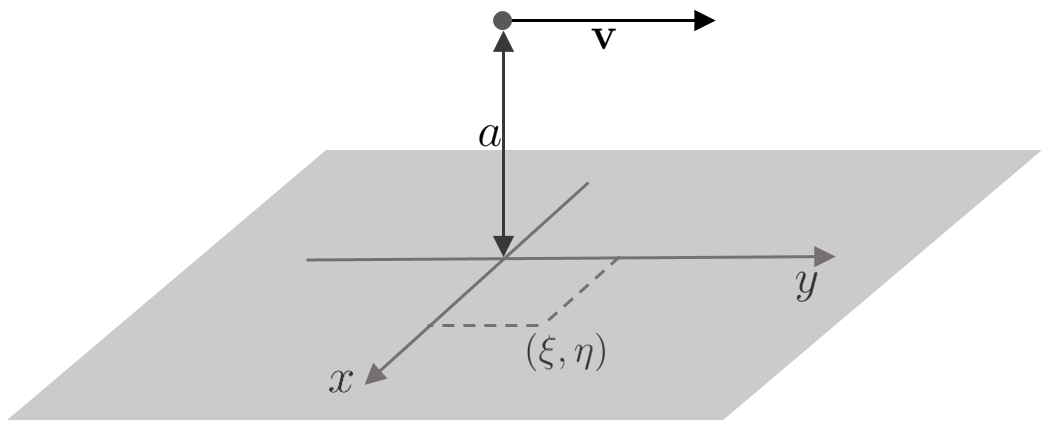
In order to study quantum friction, we consider the usual situation of the atom moving at a constant velocity, which is assumed to be parallel to the plane. Without any loss of generality, we use coordinates such that the velocity points towards the $x^{2}$ direction. Analogously, also by a proper choice of origin for space and time coordinates, the atom will pass just above the origin of the plane at $t=0$. Denoting by $a$ the (constant) distance between the atom and the plane, we then have:

$${\mathbf{r}}(t)\;=\;(0,\,vt,\,a)\;.$$

(12)

The transition amplitudes $T_{fi}=\langle f|\widehat{T}|i\rangle$ shall be determined from the scattering matrix $\widehat{S}=\hat{I}+i\widehat{T}$, namely, from the evolution operator in the interaction representation, $\widehat{U}(t_{f},t_{i})$, for $t_{i}\to-\infty$ and $t_{f}\to+\infty$:

$$\widehat{S}\;=\;\widehat{U}(+\infty,-\infty)\;=\;{\rm T}\exp[i{\mathcal{S}}^{\prime}(\hat{q},\widehat{Q},\widehat{\varphi};{\mathbf{r}}(t))\big]\;,$$

(13)

where ${\rm T}$ denotes time-ordering.

The initial quantum state $|i\rangle$ of the full system is assumed to be the vacuum for all the modes, namely, for the electron, the medium, and the vacuum field. In a self explanatory notation,

$$|i\rangle\;=\;|0_{e}\rangle\otimes|0_{m}\rangle\otimes|0_{v}\rangle\;.$$

(14)

Regarding the final state, $|f\rangle$, in quantum friction there is no production of vacuum-field particles (photons); indeed, that would require a non-vanishing acceleration. Therefore, in quantum friction, only even terms in the expansion of the exponential in (13) can intervene. The lowest order contribution to the transition amplitude is, therefore, the second order one, which yields:

$$T_{fi}\;=\;i\int d^{4}x\int d^{4}x^{\prime}\,(\langle f_{e}|\otimes\langle f_{m}|)\,\widehat{J}_{m}(x)\widehat{J}_{e}(x^{\prime})\,(|0_{e}\rangle\otimes|0_{m}\rangle)\,G(x-x^{\prime})\;,$$

(15)

where we introduced the final states for the electron and the medium, and the scalar field propagator $G$:

$$G(x-x^{\prime})\;=\;\int\frac{d^{4}k}{(2\pi)^{4}}\,e^{-ik\cdot(x-x^{\prime})}\,\frac{i}{k^{2}+i\varepsilon}\;,$$

(16)

and we have assumed the initial and final states to be normalized. It is rather straightforward to see that the only contribution to the transition amplitude (to this order) contains a quantum for both $e$ and $m$, namely:

$$|f_{e}\rangle\;=\;\hat{a}^{\dagger}|0_{e}\rangle\;\;,\;\;\;|f_{m}\rangle\;=\;\int d^{2}{\mathbf{x}}_{\shortparallel}\,f({\mathbf{x}}_{\shortparallel})\,\hat{\alpha}^{\dagger}({\mathbf{x}}_{\shortparallel})|0_{m}\rangle\;,$$

(17)

where $\int d^{2}{\mathbf{x}}_{\shortparallel}\,|f({\mathbf{x}}_{\shortparallel})|^{2}\,=\,1$. Inserting this into (15), and integrating out $x$ and $x^{\prime}$, we obtain:

$$T_{fi}\;=\;-\,\frac{2\pi g\lambda}{\sqrt{2m\Omega_{e}2\Omega_{m}}}\;\int\frac{d^{3}{\mathbf{k}}}{(2\pi)^{3}}\,\delta(\Omega_{e}+\Omega_{m}+k_{2}v)\,\frac{e^{ik^{3}a}\tilde{f^{*}}({\mathbf{k}}_{\shortparallel})}{\Omega_{m}^{2}-{\mathbf{k}}^{2}+i\varepsilon}$$

(18)

where $\tilde{f}({\mathbf{k}}_{\shortparallel})=\int d^{2}{\mathbf{x}}_{\shortparallel}\,e^{-i{\mathbf{k}}_{\shortparallel}\cdot{\mathbf{x}}_{\shortparallel}}f({\mathbf{x}}_{\shortparallel})$. Thus, integrating out $k^{2}$ and $k^{3}$, and denoting by $k_{x}\equiv k^{1}$ the only remaining component to integrate, we have that

$$T_{fi}\;=\;\frac{g\lambda}{4v\sqrt{m\Omega_{e}\Omega_{m}}}\;\int_{-\infty}^{+\infty}\frac{dk_{x}}{2\pi}\,\tilde{f^{*}}\left(k_{x},-\frac{\Omega_{e}+\Omega_{m}}{v}\right)\,\frac{e^{-a\,\sqrt{k_{x}^{2}+\Omega^{2}}}}{\sqrt{k_{x}^{2}+\Omega^{2}}}\;,$$

(19)

where we have defined

$$\Omega^{2}=\left(\frac{\Omega_{e}+\Omega_{m}}{v}\right)^{2}-\Omega_{m}^{2}\;.$$

(20)

In what follows, for the sake of notational clarity, we use denote by $x$ and $y$ the two Cartesian coordinates $x^{1}$ and $x^{2}$, respectively. We want to study the spatial properties of the transition probabilities, we consider a spatially localized function $f$, centered about a point with coordinates $(\xi,\eta)$ (see Fig. 1) on the plane, and with size $(\sigma_{x},\sigma_{y})$:

$$f(x,y)\,\equiv\,\phi_{\sigma_{x}}(x-\xi)\,\phi_{\sigma_{y}}(y-\eta)$$

(21)

where

$$\phi_{\sigma}(x)\,\equiv\,\frac{e^{-\frac{x^{2}}{4\sigma^{2}}}}{(2\pi)^{1/4}\sqrt{\sigma}}\;\;\;,\;\;\;\int_{-\infty}^{+\infty}dx\,\absolutevalue{\phi_{\sigma}(x)}^{2}\;=\;1\;.$$

(22)

Then:

	$\displaystyle T_{fi}=$	$\displaystyle\;\frac{g\lambda}{v}\sqrt{\frac{\pi\sigma_{x}\sigma_{y}}{2m\Omega_{e}\Omega_{m}}}\,e^{-\sigma^{2}_{y}\left(\frac{\Omega_{e}+\Omega_{m}}{v}\right)^{2}}\;e^{i\eta(\frac{\Omega_{e}+\Omega_{m}}{v})}$
		$\displaystyle\times\int_{-\infty}^{+\infty}\,\frac{dk_{x}}{2\pi}\,e^{-\sigma_{x}^{2}k_{x}^{2}}\,e^{-ik_{x}\xi}\frac{e^{-a\,\sqrt{k_{x}^{2}+\Omega^{2}}}}{\sqrt{k_{x}^{2}+\Omega^{2}}}\;.$		(23)

Note that $\rho(\xi)\;\equiv\;|T_{fi}|^{2}/\sigma_{x}\sigma_{y}$ is a probability per unit area, and making $\sigma_{x},\sigma_{y}\to 0$ would give the probability (per area) of having an oscillator of the medium excited at $(\xi,\eta)$¹¹ 1 This is equivalent to taking $f({\mathbf{x}}_{\shortparallel})\propto\delta(x-\xi)\delta(y-\eta)$ in (17).

$$\rho(\xi)\equiv\lim_{\sigma_{x},\sigma_{y}\to 0}\frac{|T_{fi}|^{2}}{\sigma_{x}\sigma_{y}}=\frac{g^{2}\lambda^{2}}{8\pi m\Omega_{m}\Omega_{e}v^{2}}\absolutevalue{\int_{-\infty}^\infty dk_x~e^{-ik_x\xi} \frac{e^{- a \,\sqrt{ k_x^2 + \Omega^2}}}{\sqrt{ k_x^2 + \Omega^2}}}^{2}\;,$$

(24)

which does not depend on $\eta$.

With $\Omega$ as defined in (20), and giving different values to the adimensional combination $\Omega a$ for fixed $\Omega_{e}$, we can see in the Fig.2 how this distribution varies with the distance between the medium and the atom, and with the quotient $f\equiv\Omega_{m}/\Omega_{e}$.

Integrating $\rho(\xi)$ for all $\xi$ and multiplying by a characteristic length in the direction of movement of the atom, i.e. $vT$, where we can think of $T$ as the time the atom has been moving with constant speed $v$, gives the probability of this process to happen. Then, dividing by $T$, would give the probability per unit time

$$\mathcal{P}\equiv\frac{1}{T}\penalty\ vT\int_{-\infty}^{\infty}d\xi\penalty\ \rho(\xi)=\frac{g^{2}\lambda^{2}}{2mv\Omega_{e}\Omega_{m}}\int_{0}^{\infty}\,\,dk_{x}\penalty\ \frac{e^{-2a\sqrt{k_{x}^{2}+(\frac{\Omega_{e}+\Omega_{m}}{v})^{2}-\Omega_{m}^{2}}}}{k_{x}^{2}+(\frac{\Omega_{e}+\Omega_{m}}{v})^{2}-\Omega_{m}^{2}},$$

(25)

which matches with the result obtained in equation (69) of [6].

Now we consider the case where waves can be propagated through the medium at speed $u\neq 0$, and see that results match with the previous model when $u\to 0$. The action for the medium is now

$${\mathcal{S}}^{(0)}_{m}(Q)\,=\,\int d^{3}x_{\shortparallel}\,\frac{1}{2}\left[\big(\partial_{t}Q(x_{\shortparallel})\big)^{2}\,-\,u^{2}\,\big|{\mathbf{\nabla}}_{\shortparallel}Q(x_{\shortparallel})\big|^{2}\,-\,\Omega_{m}^{2}Q^{2}(x_{\shortparallel})\right],$$

(26)

and the second expression of (3) turns into

$$\hat{Q}(x_{\shortparallel})=\;\int\frac{d^{2}{\mathbf{k}}_{\shortparallel}}{2\pi}\frac{1}{\sqrt{2k_{0}}}\big(\hat{\alpha}({\mathbf{k}}_{\shortparallel})\,e^{-ik_{\shortparallel}\cdot x_{\shortparallel}}\,+\,\hat{\alpha}^{\dagger}({\mathbf{k}}_{\shortparallel})\,e^{ik_{\shortparallel}\cdot x_{\shortparallel}}\big),$$

(27)

where $k_{0}=\sqrt{u^{2}\absolutevalue{\mathbf{k}_\shortparallel}^{2}+\Omega_{m}^{2}}$ and $[\hat{\alpha}({\mathbf{k}}_{\shortparallel})\,,\,\hat{\alpha}^{\dagger}({\mathbf{p}}_{\shortparallel})]\,=\,\delta^{2}({\mathbf{k}}_{\shortparallel}-{\mathbf{p}}_{\shortparallel})$. The (normalized) final state that we consider now is $\ket{f_m}=\frac{2\pi}{\ell}\alpha^{\dagger}({\mathbf{p}}_{\shortparallel})\ket{0_m}$, i.e. an excitation with momentum $\mathbf{p}_{\shortparallel}$.²² 2 When $u=0$, this is equivalent to taking $f({\mathbf{x}}_{\shortparallel})\propto e^{-i\mathbf{p}_{\shortparallel}\cdot{\mathbf{x}}_{\shortparallel}}$ in (17). This gives a transition amplitude

	$\displaystyle T_{fi}=$	$\displaystyle\frac{2\pi}{\ell}\frac{g\lambda\penalty\ e^{-a\sqrt{\absolutevalue{\mathbf{p}_\shortparallel}^{2}(1-u^{2})-\Omega_{m}^{2}}}}{\sqrt{m\Omega_{e}\left(\absolutevalue{\mathbf{p}_\shortparallel}^{2}(1-u^{2})-\Omega_{m}^{2}\right)\sqrt{u^{2}\absolutevalue{\mathbf{p}_\shortparallel}^{2}+\Omega_{m}^{2}}}}$
		$\displaystyle\times\delta\left(\Omega_{e}+\sqrt{u^{2}\absolutevalue{\mathbf{p}_\shortparallel}^{2}+\Omega_{m}^{2}}-vp_{y}\right).$		(28)

The arising Dirac delta gives us some information about the process. First, $p_{y}$ has to be positive, so the momentum of the excitation in the medium has a positive component along the velocity of the atom. Then, it shows that there is a threshold for this process to occur: the speed of the atom should be greater than the speed of the waves propagating in the medium $v>u$.

$$up_{y}<u\absolutevalue{\mathbf{p}_\shortparallel}<\sqrt{u^{2}\absolutevalue{\mathbf{p}_\shortparallel}^{2}+\Omega_{m}^{2}}=vp_{y}$$

(29)

Dividing $\absolutevalue{T_{fi}}^{2}$ by $T$ with $u\to 0$ and integrating all possible momentums for the excitation of the medium gives the probability per unit time of having this process.

$$\mathcal{P}=\frac{1}{T}\left(\frac{\ell}{2\pi}\right)^{2}\int d^{2}\mathbf{p}_{\shortparallel}\penalty\ \lim_{u\to 0}\absolutevalue{T_{fi}}^{2}=\frac{g^{2}\lambda^{2}}{\pi mv\Omega_{e}\Omega_{m}}\int_{0}^{\infty}dp_{x}\frac{e^{-2a\sqrt{p_{x}^{2}+(\frac{\Omega_{e}\Omega_{m}}{v})^{2}-\Omega_{m}^{2}}}}{p_{x}^{2}+(\frac{\Omega_{e}+\Omega_{m}}{v})^{2}-\Omega_{m}^{2}},$$

(30)

which is essentially the same as (25).

In this paper, we have evaluated the transition amplitudes corresponding to the elementary processes which lead to the phenomenon of quantum friction between a moving atom and a material plane. Our choice of system, and model, allows for a determination of the spatial dependence of the Casimir friction phenomenon, by providing the funcional form of the amplitude as a function of the distance, on the plane, to the projection of the atom’s trajectory.

The dependence of the previous results on the distance between the atom and the plane is modulated by a precise combination of the model’s parameters and the velocity of the atom.

Finally, by integrating out the probabilities to this order, we have found agreement with the total vacuum decay probability obtained, for the same model, by an evaluation of the imaginary part of the effective action, in a functional integral approach.

The authors thank ANPCyT, CONICET, CNEA and UNCuyo for financial support.

References

- [1] P.W. Milonni, The Quantum Vacuum (Academic Press, San Diego, 1994); M. Bordag, U. Mohideen, and V.M. Mostepanenko, Phys. Rep. 353, 1 (2001); K. A. Milton, The Casimir Effect: Physical Manifestations of the Zero- Point Energy (World Scientific, Singapore, 2001); S. Reynaud, A. Lambrecht, C. Genet, and M.T. Jaekel, et al., C. R. Acad. Sci. Paris Ser. IV 2, 1287 (2001); K. A. Milton, J. Phys. A 37, R209 (2004); S. K. Lamoreaux, Rep. Prog. Phys. 68, 201 (2005); M. Bordag, G. L. Klimchitskaya, U. Mohideen, and V. M. Mostepanenko, Advances in the Casimir Effect (Oxford University Press, Oxford, 2009).
- [2] J.B. Pendry, J. Phys.:Condens. Matter 9, 10301 (1997).
- [3] M. F. Maghrebi, R. Golestanian and M. Kardar, Phys. Rev. A 88, 042509 (2013).
- [4] C. D. Fosco, F. C. Lombardo and F. D. Mazzitelli, Universe 7, no.5, 158 (2021).
- [5] J.S. Hoye and Brevik I., EPL, 91, 60003 (2010); ibidem Europ. Phys. J. D, in press (arXiv:1009.3135 v2); G. Barton, New J. Phys. 12, 113044 (2010); ibidem New J. Phys. 12, 113045 (2010).
- [6] M. B. Farías, C. D. Fosco, F. C. Lombardo and F. D. Mazzitelli, Phys. Rev. D 100, no.3, 036013 (2019).
- [7] C. R. Galley, R. O. Behunin and B. L. Hu, Phys. Rev. A 87, 043832 (2013).
- [8] C. D. Fosco, F. C. Lombardo and F. D. Mazzitelli, Phys. Rev. D 84, 025011 (2011).
- [9] C. D. Fosco, F. C. Lombardo and F. D. Mazzitelli, Phys. Rev. D 76, 085007 (2007).
- [10] M. Belén Farías, C. D. Fosco, F. C. Lombardo, F. D. Mazzitelli and A. E. Rubio López, Phys. Rev. D 91, no.10, 105020 (2015).
- [11] J. S. Schwinger, J. Math. Phys. (N.Y.) 2, 407 (1961); L. V. Keldysh, Zh. Eksp. Teor. Fiz. 47, 1515 (1965) [Sov. Phys. JETP 20, 1018 (1965)] E. A. Calzetta and B. L. Hu, Nonequilibriium Quantum Field Theory (Cambridge University Press, Cambridge, England, 2008).