A General Analytical Approach for Outage Analysis of HARQ-IR over Correlated Fading Channels
Abstract
This paper proposes a general analytical approach to derive the outage probability of hybrid automatic repeat request with incremental redundancy (HARQ-IR) over correlated fading channels in closed-form. Unlike prior analyses, the consideration of channel correlation is one of the key reasons making the outage analysis involved. Using conditional Mellin transform, the outage probability of HARQ-IR over correlated Rayleigh fading channels is exactly expressed as a mixture of outage probabilities of HARQ-IR over independent Nakagami fading channels, where the weights are negative multinomial probabilities. Its straightforward application is to conduct asymptotic outage analysis to gain more insights, in which the asymptotic outage probability is obtained in a concise form. The asymptotic outage probability possesses some special properties which ease optimal power allocation and rate selection of HARQ-IR. Finally, numerical results are presented for validations and discussions.
Index Terms:
hybrid automatic repeat request with incremental redundancy, correlated Rayleigh fading, Mellin transform.I Introduction
In the last decade we have witnessed an ever increasing research interest in hybrid automatic repeat request (HARQ) owing to its high potential for reliable reception. It has been rigorously proved in [1] that HARQ with incremental redundancy (HARQ-IR) can reach the ergodic capacity in Gaussian collision channels. Moreover, HARQ-IR outperforms other types of HARQ (i.e., Type I HARQ and HARQ with chase combining) since extra coding gain is achieved.
Although HARQ-IR has been studied extensively in the literature, most of them assume either quasi-static [2, 3] or independent fading channels [4, 5, 6, 7, 8]. For example, [2] and [3] conduct average rate performance analysis and power optimization for HARQ-IR, respectively, under quasi-static fading channels. The quasi-static fading channels assume the same channel realization experienced in all HARQ rounds. However, the analytical results under quasi-static fading channels only apply to low mobility environment. In contrast, the transmitted signals in high mobility environment usually undergo independent fading channels, where the channels are assumed to vary independently from one transmission to another. In this scenario, the analysis becomes to determine the cumulative distribution function (CDF) of the product of multiple shifted independent random variables (RVs). Several approaches have been developed to handle this problem in the literature. For example, in [4], Log-normal approximation is proposed based on central limit theorem (CLT). Nevertheless, this approximation can not ease the optimal system design because of the complex results. Moreover, [5] adopts Jensen’s inequality to obtain the lower bound of the CDF to reduce the computational complexity. In order to obtain the exact CDF, two methods are developed, i.e., Mellin transform [6, 7] and multi-fold convolution [8]. Unfortunately, the analytical results obtained from the two methods are too complicated to apply to optimal design.
In addition, another widely adopted channel model is correlated fading channel, which usually occurs in low-to-medium mobility environment. To our best knowledge, only few approximation approaches have been proposed to analyze the performance of HARQ-IR over time-correlated fading channels, i.e., Log-normal approximation [9], polynomial fitting technique [10], inverse moment matching method [11] and Jensen’s inequality [12]. Unfortunately, Log-normal approximation in [9] is inaccurate under fading channels with medium-to-high correlation. To improve the approximation accuracy, other two approximation approaches are developed in [10, 11]. However, the proposed approximation approaches admit a mean square error (MSE) convergence, which does not necessarily imply that the approximation error would approach to zero at every point [13, p86]. Particularly, the proposed approximation approaches become unstable when evaluating a low outage probability, which limits their application to conducting the asymptotic outage analysis to further extract insightful results. Besides, the analytical results in [10, 11] are still too complicated to apply to practical system design. To avoid that, a tractable approximate expression is derived for outage probability based on Jensen’s inequality, and is then applied to obtain optimal transmission powers in closed-form in [12]. However, there exists an evident gap between the approximate and the exact optimal solutions.
In this paper, a general analytical approach is proposed to derive the outage probability of HARQ-IR over exponentially correlated Rayleigh fading channels. By using conditional Mellin transform, the outage probability is exactly derived as a representation of a mixture of outage probabilities of HARQ-IR over independent Nakagami fading channels where the weights are negative multinomial probabilities. The analytical result, of independent interest, facilitates asymptotic outage analysis. Specifically, the asymptotic outage probability is derived in a compact form which clearly quantifies the impacts of channel time correlation, transmission rate and powers. Moreover, the special properties of asymptotic outage probability facilitate the optimal system design.
The rest of this paper is structured as follows. Section II introduces the system model and formulates the outage probability of HARQ-IR. Exact and asymptotic outage analyses are conducted in Section III and IV, respectively. Section V verifies our numerical results. Finally, some conclusions are drawn in Section VI.
II System Model and Outage Formulation
Due to space limitation, this paper considers a point-to-point HARQ-IR enabled system operating over exponentially correlated Rayleigh fading channels. It is worth emphasizing that the general analytical approach proposed in this paper can be easily applied to more complicated HARQ-IR system. To facilitate outage formulation, HARQ-IR protocol and time-correlated fading channels are first introduced.
II-A HARQ-IR protocol
Following HARQ-IR, each original information message is first encoded into sub-codewords at the source, where denotes the maximum allowable number of transmissions for each message. These sub-codewords will be delivered one by one until the message is successfully decoded. In each transmission, all the erroneously received sub-codewords are combined with currently received sub-codewords for joint decoding. If success, an acknowledgement (ACK) message is fed back to the source and the transmission for the next information message will be initiated. Otherwise, a negative acknowledgement (NACK) message is fed back to notify the source, and the next sub-codeword is transmitted until the maximum number of transmissions is reached.
II-B Time-correlated Rayleigh fading channels
Denote as the th sub-codeword of length . We assume a block fading channel, the signal received in the th transmission is thus given by
| (1) |
where denotes a complex additive white Gaussian noise (AWGN) vector with mean vector and covariance matrix , i.e., , represents an identity matrix, denotes the block Rayleigh fading channel coefficient in the th transmission. In this paper, time correlation of fading channels is considered. A commonly adopted correlated Rayleigh fading channel model is given as [14]
| (2) |
where , and denote the time correlation, the channel feedback delay and the mean squared magnitude of , respectively; and are independent circularly-symmetric complex normal RVs with zero mean and unit variance, i.e., .
According to (1), the received signal-to-noise ratio (SNR) in the th transmission is
| (3) |
where is the transmitted signal power in the th transmission. Since the channel magnitude is Rayleigh distributed, complies with exponential distribution with mean . Due to the correlation between fading channels, the SNRs are thus correlated exponential RVs.
II-C Outage Formulation
Outage probability is proved as the most fundamental performance metric of HARQ schemes [1]. Specifically, assuming that information-theoretic capacity achieving channel coding is adopted for HARQ-IR, an outage event happens when the accumulated mutual information is below the transmission rate . The outage probability after transmissions is thus written as
| (4) |
where denotes the CDF of . Following the HARQ-IR protocol, the accumulated mutual information after transmissions is given by
| (5) |
Accordingly, the outage probability becomes as
| (6) |
where denotes the CDF of . Therefore, noting that are correlated exponential RVs, the derivation of outage probability essentially turns to determining the CDF of the product of multiple shifted correlated-exponential RVs, i.e., .
III Exact Outage Analysis
Unlike the outage analysis under independent fading channels [4, 5, 6, 7, 8], it is more challenging to derive an exact expression for outage probability when fading channels are time-correlated. Recall that the derivation of essentially turns to determining the CDF of the product of multiple shifted correlated-exponential RVs, i.e., . To the best of our knowledge, there is no readily available method to solve the problem. Nevertheless, it is found from (3) that correlation among the SNRs can be eliminated given the RV , i.e., the SNRs are independent when is given. This conditional independence of SNRs inspires us to derive the CDF of using conditional Mellin transform. Specifically, it can be proved by using [15, Theorem 1.3.4] that follows independent noncentral chi-squared distributions with degrees-of-freedom conditioned on . The conditional PDF of the SNR given is given by
| (7) |
where denotes the confluent hypergeometric limit function [16, Eq.9.14.1], and .
Noticing that Mellin transform is an efficient way to obtain the distribution of a product of multiple independent RVs, the conditional Mellin transform is proposed to derive the conditional probability density function (PDF) of given as follows.
When given , the Mellin transform with respect to the conditional PDF of , , can be written as
| (8) |
where denotes Tricomi’s confluent hypergeometric function [16, 9.211,4].
Accordingly, by using inverse Mellin transform, can be written as [17]
| (9) |
where . Putting (8) into (9), it yields
| (10) |
where and denotes the PDF of the product of independent shifted-Gamma RVs, i.e., , and . is explicitly given by (III), as shown at the top of next page,
With (10), the PDF of can then be obtained by averaging the conditional probability over the distribution of , such that
| (13) |
where denotes the PDF of . Since is a complex Gaussian RV with zero mean and unit variance, obeys a exponential distribution with the PDF of
| (14) |
Substituting (10) and (14) into (13), the following theorem can be obtained after some mathematical manipulations.
Theorem 1.
The PDF of can be expressed as a mixture of PDFs of products of independent shifted-Gamma RVs, such that
| (15) |
where denotes -ary Cartesian power of natural number set; follows a negative multinomial distribution whose probability mass function (pmf) is
| (16) |
with , , and , i.e., .
Proof.
The detailed derivation is omitted due to space limitation. ∎
Accordingly, the CDF of can be derived based on (15), as shown in the following corollary.
Corollary 1.
The CDF of is given by
| (17) |
where denotes the CDF of a product of independent shifted-Gamma RVs , and can be expressed in terms of Fox’s H function as (1), as shown at the top of next page.
It follows from (6) and (17) that the outage probability can be written as
| (20) |
Furthermore, meaningful results can be extracted from (20), as given in the following remark.
Remark 1.
In fact, can be regarded as an outage probability of HARQ-IR after transmissions over independent Nakagami-m fading channels, where and denotes the corresponding channel coefficient in the th transmission, i.e.,
| (21) |
Therefore, the outage probability can be treated as a mixture of outage probabilities of HARQ-IR over independent Nakagami fading channels where the weights are probabilities of .
The result in Remark 1 is very useful in the later asymptotic outage analysis.
IV Asymptotic Outage Analysis
IV-A Asymptotic Outage Probability
Although outage probability of HARQ-IR over time-correlated fading channels can be derived in closed-form in (20), straightforward insights still can not be found. Therefore, the asymptotic analysis of outage probability is resorted to extract meaningful insights for HARQ-IR. To proceed, we assume that
| (22) |
where denotes a constant vector associated with power allocation. Noticing that is a weighted sum of , some asymptotic properties with respect to are proved first under high SNR regime, i.e., , to facilitate the asymptotic analysis of . Due to the independence of RVs , the asymptotic expression of as can be derived. Specifically, from (1), can be written in the form of Mellin-Barnes integral, such that
| (23) |
where and . By adopting [16, Eq.9.210.2], it produces
Since can be expanded as
| (26) |
where refers to the little-O notation, and we say provided that . Clearly, as approaches to infinity, the dominant term in (26) is .
Herein, we assume because could be any point in . Therefore, (IV-A) can be further written as
| (27) |
where . After some manipulations, can be finally expressed as
| (28) |
According to (28), it is readily found that the following lemma holds.
Lemma 1.
As , the ratio of to satisfies
| (29) |
This lemma will enable the derivation of the asymptotic outage probability . Specifically, with Lemma 1, the CDF can be written as
| (30) |
where the last step holds since is irrelevant to and .
With (28), (IV-A) can be further simplified as
| (31) |
where is a function of and , such that
| (32) |
and
| (35) |
where denotes the residue of at . Substituting (31) into (20) along with (22), the asymptotic outage probability can be derived, as shown in the following theorem.
Theorem 2.
The asymptotic outage probability can be decoupled as
| (36) |
where . The impacts of transmission rate, channel time correlation and transmit powers on outage probability are clearly quantified through the terms of , and , respectively.
It is noteworthy that the asymptotic outage probability of HARQ-IR has never been accurately derived even under independent fading channels, which justifies the significance of our work.
IV-B Discussions
IV-B1 Impact of Transmission Power
It is shown in (36) that the asymptotic outage probability is influenced by the product of transmission powers in all HARQ rounds, i.e., . Therefore, the optimal power allocation for HARQ-IR over time-correlated fading channels can be enabled by adopting the same method developed in [18]. For more details about optimal power allocation of HARQ, please consult with [18].
IV-B2 Effect of Transmission Rate
Clearly from (36), the impact of transmission rate on asymptotic outage probability is determined by . With (IV-A), it can be proved that the first and the second derivative of with respect to are non-negative, more precisely
| (37) |
| (38) |
Thus is an increasing and convex function of , which will greatly facilitate the optimal rate selection with numerous sophisticated convex methods.
V Numerical Results
In this section, analytical results are verified. For illustration, we take systems with , , and as examples. Notice that the exact outage probability in (20) is calculated approximately by truncating the infinite series into a finite series with the constraint of . In the following numerical analysis, the truncation order is set as .
In Fig. 1, the exact and asymptotic outage probabilities are plotted against transmit power by setting . Clearly, the exact results perfectly match with the simulation results and the asymptotic results coincide well with the exact/simulation results under high transmit power , which justify the correctness of our analysis. For comparison, the outage probabilities obtained by using polynomial fitting technique [10] are also presented in Fig. 1. It can be seen that polynomial fitting technique does not provide a good approximation under high SNR regime due to the inability to guarantee the pointwise convergence. Thus this comparison further highlights the significance of the asymptotic outage analysis. In addition, note that diversity order quantifies the slope of outage probability against transmit power in a log-log scale. It is observed from Fig. 1 that curves under different time correlation become parallel as increases, which is consistent with our conclusion that time correlation does not influence diversity order.

As shown in Fig. 2, is plotted against transmission rate under different maximum numbers of transmissions . As expected, is an increasing and convex function of , which justifies the correctness of our analysis.
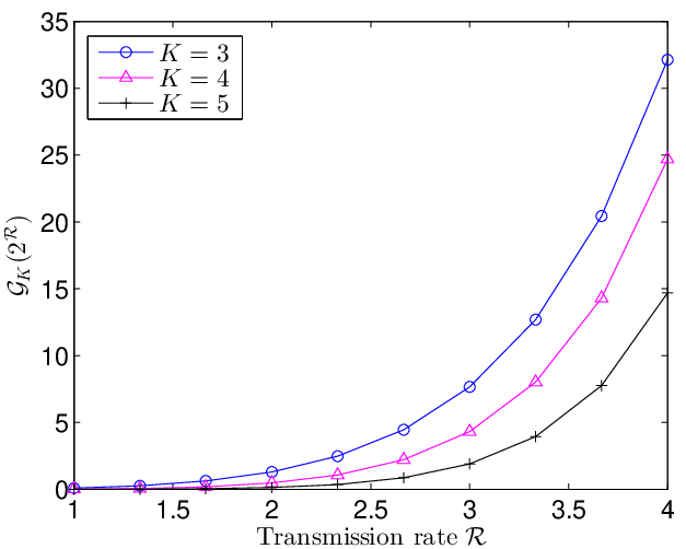
Fig. 3 illustrates the effect of time correlation on the outage probability of HARQ-IR by setting dB. It is readily found that the simulation results agree with the analytical results very well. In addition, it is verified that time correlation adversely affects the outage performance.

VI Conclusions
In this paper, exact and asymptotic outage probabilities of HARQ-IR over time-correlated Rayleigh fading channels have been analyzed by developing a general analytical approach. In particular, the asymptotic outage probability has been derived in a simple form with which the impacts of time correlation, transmission rate and transmit powers are clearly quantified. The special form of asymptotic outage probability also eases the optimal system design, e.g., optimal power allocation and optimal rate selection.
VII Acknowledgements
This work was supported in part by National Natural Science Foundation of China under grants 61601524 and 61671488, in part by the Special Fund for Science and Technology Development in Guangdong Province under Grant No. 2016A050503025, in part by the Research Committee of University of Macau under grants MYRG2014-00146-FST and MYRG2016-00146-FST, and in part by the Macau Science and Technology Development Fund under grants 091/2015/A3 and 020/2015/AMJ.
References
- [1] G. Caire and D. Tuninetti, “The throughput of hybrid-ARQ protocols for the Gaussian collision channel,” IEEE Trans. Inf. Theory, vol. 47, no. 5, pp. 1971–1988, Jul. 2001.
- [2] C. Shen, T. Liu, and M. P. Fitz, “On the average rate performance of hybrid-ARQ in quasi-static fading channels,” IEEE Trans. Commun., vol. 57, no. 11, pp. 3339–3352, Nov. 2009.
- [3] B. Makki, A. Graell i Amat, and T. Eriksson, “Green communication via power-optimized HARQ protocols,” IEEE Trans. Veh. Technol., vol. 63, no. 1, pp. 161–177, Jan. 2014.
- [4] D. To, H. X. Nguyen, Q.-T. Vien, and L.-K. Huang, “Power allocation for HARQ-IR systems under QoS constraints and limited feedback,” IEEE Trans. Wireless Commun., vol. 14, no. 3, pp. 1581–1594, Mar. 2015.
- [5] J. Choi, W. Xing, D. To, Y. Wu, and S. Xu, “On the energy efficiency of a relaying protocol with HARQ-IR and distributed cooperative beamforming,” IEEE Trans. Wireless Commun., vol. 12, no. 2, pp. 769–781, Feb. 2013.
- [6] F. Yilmaz and M.-S. Alouini, “Product of shifted exponential variates and outage capacity of multicarrier systems,” in Proc. European Wireless Conference (EW’09), May 2009, pp. 282–286.
- [7] A. Chelli and M. Alouini, “On the performance of hybrid-ARQ with incremental redundancy and with code combining over relay channels,” IEEE Trans. Wireless Commun., vol. 12, no. 8, pp. 3860–3871, Aug. 2013.
- [8] P. Larsson, L. K. Rasmussen, and M. Skoglund, “Throughput analysis of ARQ schemes in Gaussian block fading channels,” IEEE Trans. Commun., vol. 62, no. 7, pp. 2569–2588, Jul. 2014.
- [9] X. Yang, Z. Shi, S. Ma, and K.-W. Tam, “Performance analysis of cooperative HARQ-IR over time-correlated Nakagami-m fading channels,” in Proc. IEEE International Conference on Communication Systems (ICCS’14), Nov. 2014, pp. 404–408.
- [10] Z. Shi, H. Ding, S. Ma, and K.-W. Tam, “Analysis of HARQ-IR over time-correlated Rayleigh fading channels,” IEEE Trans. Wireless Commun., vol. 14, no. 12, pp. 7096–7109, Dec. 2015.
- [11] Z. Shi, H. Ding, S. Ma, K.-W. Tam, and S. Pan, “Inverse moment matching based analysis of cooperative HARQ-IR over time-correlated Nakagami fading channels,” IEEE Trans. Veh. Technol., vol. PP, no. 99, pp. 1–1, 2016.
- [12] Z. Shi, S. Ma, F. Hou, K.-W. Tam, and Y.-C. Wu, “Optimal power allocation for HARQ schemes over time-correlated nakagami-m fading channels,” in Proc. IEEE International Conference on Communication Systems (ICCS’16). IEEE, 2016, pp. 1–6.
- [13] M. Adams, Continuous-Time Signals and Systems. University of Victoria, 2013. [Online]. Available: https://books.google.com/books?id=RQI9ngEACAAJ
- [14] S. M. Kim, W. Choi, T. W. Ban, and D. K. Sung, “Optimal rate adaptation for hybrid ARQ in time-correlated Rayleigh fading channels,” IEEE Trans. Wireless Commun., vol. 10, no. 3, pp. 968–979, Mar. 2011.
- [15] R. J. Muirhead, Aspects of multivariate statistical theory. John Wiley & Sons, 2009, vol. 197.
- [16] I. S. Gradshteyn, I. M. Ryzhik, A. Jeffrey, D. Zwillinger, and S. Technica, Table of integrals, series, and products. Academic press New York, 1965, vol. 6.
- [17] L. Debnath and D. Bhatta, Integral transforms and their applications. CRC press, 2010.
- [18] T. Chaitanya and T. Le-Ngoc, “Energy-efficient adaptive power allocation for incremental MIMO systems,” IEEE Trans. Veh. Technol., vol. PP, no. 99, pp. 1–1, 2015.