- AE
- autoencoder
- AI
- artificial intelligence
- AoA
- angle-of-arrival
- AoD
- angle-of-departure
- BS
- base station
- BP
- belief propagation
- CDF
- cumulative density function
- CRB
- Cramér-Rao bound
- DA
- data association
- D-MIMO
- distributed multiple-input multiple-output
- DL
- downlink
- EM
- electromagnetic
- E2E
- end-to-end
- FIM
- Fisher information matrix
- GDOP
- geometric dilution of precision
- GNSS
- global navigation satellite system
- GPS
- global positioning system
- HWI
- hardware impairment
- IP
- incidence point
- IQ
- in-phase and quadrature
- ISAC
- integrated sensing and communication
- ICI
- inter-carrier interference
- JCS
- Joint Communication and Sensing
- JRC
- joint radar and communication
- JRC2LS
- joint radar communication, computation, localization, and sensing
- IMU
- inertial measurement unit
- IOO
- indoor open office
- IoT
- Internet of Things
- IRN
- infrastructure reference node
- KPI
- key performance indicator
- LoS
- line-of-sight
- LS
- least-squares
- MC
- mutual coupling
- MCRB
- misspecified Cramér-Rao bound
- MIMO
- multiple-input multiple-output
- MISO
- multiple-input single-output
- ML
- maximum likelihood
- mmWave
- millimeter-wave
- MSE
- mean squared error
- NLoS
- non-line-of-sight
- NN
- neural network
- NR
- new radio
- OFDM
- orthogonal frequency-division multiplexing
- OTFS
- orthogonal time-frequency-space
- OEB
- orientation error bound
- PEB
- position error bound
- VEB
- velocity error bound
- PRS
- positioning reference signal
- QoS
- Quality of Service
- RAN
- radio access network
- RAT
- radio access technology
- RCS
- radar cross section
- RedCap
- reduced capacity
- RF
- radio frequency
- RIS
- reconfigurable intelligent surface
- RFS
- random finite set
- RMSE
- root mean squared error
- RTK
- real-time kinematic
- RTT
- round-trip-time
- SLAM
- simultaneous localization and mapping
- SLAT
- simultaneous localization and tracking
- SNR
- signal-to-noise ratio
- ToA
- time-of-arrival
- TDoA
- time-difference-of-arrival
- TR
- time-reversal
- TX/RX
- transmitter/receiver
- Tx
- transmitter
- Rx
- receiver
- UE
- user equipment
- UL
- uplink
- ULA
- uniform linear array
- UWB
- ultra wideband
- XL-MIMO
- extra-large MIMO
- NLL
- negative log-likelihood
Spatial Signal Design for Positioning via End-to-End Learning
Abstract
This letter considers the problem of E2E (E2E) learning for joint optimization of transmitter precoding and receiver processing for mmWave downlink positioning. Considering a MISO (MISO) scenario, we propose a novel AE (AE) architecture to estimate UE (UE) position with multiple BS and demonstrate that E2E learning can match model-based design, both for AoD (AoD) and position estimation, under ideal conditions without model deficits and outperform it in the presence of hardware impairments.
Index Terms:
mmWave positioning, precoder optimization, end-to-end learning.I Introduction
The combination of high delay resolution at mmWave frequencies thanks to large bandwidth and high angular resolution thanks to large arrays is an important enabler for accurate positioning in 5G [1] and beyond [2]. The estimation of ToA (ToA), AoA (AoA), and AoD (AoD) is enabled by designed pilot signals in time, frequency, and in space (at the BS (BS)) [3]. Such designs, in combination with advanced signal processing, can leverage the physical resources efficiently when suitable models are available. Traditionally, signal designs were optimized for broadcast performance in order to localize all users irrespective of their position [4]. Recently, there has been an increased focus on spatial per-user signal design, leveraging a priori knowledge of the user’s location in order to further improve accuracy, both for positioning [5] and sensing [6]. Signal designs can be categorized as model-based [7, 5, 8, 9, 10] or based on AI (AI) [11, 12, 13, 14]. Model-based signal designs can be performed based on simple heuristics [7], or on minimizing the CRB (CRB) on the AoA, AoD, or the position via the PEB (PEB). After relaxation, the optimization problems can be cast in convex forms, leading to elegant and efficient designs (e.g., [5] for angle estimation and [10] for positioning). From these solutions, online adaptive precoders [8] and robust designs based on predetermined codebooks with power allocation [9] have been considered.
An important limitation of model-based designs is that they require a model of the transmitter, receiver, and propagation channel. Under model mismatch, e.g., HWI, model-based approaches may exhibit degraded performance. Moreover, in certain cases, even with perfect model knowledge, finding optimal signal designs can be intractable. To remedy these two shortcomings, E2E learning has been gaining interest, first in the context of communication [15] and more recently for sensing [11], but not for positioning. The principle is to model the entire system as an AE [15] or by a combination or a reinforcement learning transmitter and a supervised learning receiver [16], combined with a suitable loss function (see, e.g., [11]). An application of E2E learning for spatial precoder design can be found in [12], where the probing codebook is implemented by a NN (NN) module that is jointly trained with the beam predictor in order to predict the optimal narrow beam. Furthermore, [13] extends the learned beamforming to ISAC (ISAC) by implementing the transmitter as a convolutional NN able to learn the features of historical channel and predict the next beamforming matrix. E2E learning in the presence of HWI for ISAC has been proposed in [14]. AI-based solutions have also been applied in other forms to deal with HWI, e.g., [17] proposes a super-resolution direction of arrival network, implemented as a convolutional NN, that can outperform AoA estimation methods under MC (MC).
In this paper, E2E learning is applied for the first time in positioning, in order to jointly optimize transmit beamformers and receiver-side algorithms, even in the presence of HWI. Our contributions are (i) a novel AE architecture and loss function for AoD- and positioning-optimized signal design and estimator design; (ii) a detailed performance comparison to a state-of-the-art model-based benchmark and corresponding CRB; (iii) an evaluation under different HWI, namely array element inter-distance perturbation and array MC, demonstrating the robustness of the proposed E2E solution.
II System Model
II-A Scenario and Signal Model
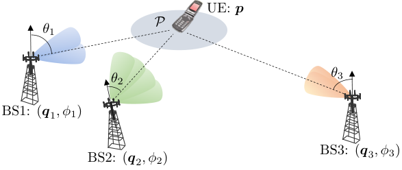
We consider a mmWave MISO downlink scenario with multiple-antenna BS and a single-antenna UE with unknown location , where is the prior location information. Each BS has a known location and orientation , and is assumed to be equipped with an -element ULA (ULA) with antenna spacing, where denotes the wavelength of the carrier. The scenario is visualized in Fig. 1.
The -th BS broadcasts a narrowband signal over successive transmissions. We assume that BS transmissions are orthogonalized in time or frequency [4], leading to the observation at the UE from BS at transmission given by
| (1) |
where denotes the pilot signal with an unit power , and denote, respectively, the complex channel gain and AoD from the -th BS, is the array steering vector at the BS (ULA of elements and antenna spacing), is the precoder employed by the -th BS at time , and is the additive white noise with variance , accounting also for the signal energy. In a more compact form, (1) can be rewritten as
| (2) |
where represents the Hadamard product, , is the precoder matrix of the -th BS, , and . From the UE and BS positions, the AoD is computed as
| (3) |
which accounts for the BS orientation. We assume that the UE lies in the angular sector with respect to the BS , depending on the uncertainty region .
II-B Hardware Impairment Models
Without HWI, the steering vectors are given by , . We now describe the impact of inter-antenna element spacing perturbations and MC, which lead to an impaired steering vector, denoted by .
II-B1 Antenna Element Spacing Perturbations
We introduce the vector of inter-element distances as , where without HWIs, . Here, denotes a vector of ones. With spacing perturbations caused by HWIs [18], the distance is modeled by
| (4) |
so that the perturbed steering vector becomes .
II-B2 Mutual Coupling
Following [19], we introduce a coupling matrix , which is modeled as a banded symmetric Toeplitz matrix whose entries are collected in the vector , where is the number of half-wavelength increments for which the MC contribution is assumed non-negligible, so that .
III End-to-End Learning
In this section, we describe the proposed architectures, the associated loss functions, and the model-based benchmark.
III-A End-to-End Learning Architecture
We consider two separate AE architectures for AoD and position estimation, as shown in Fig. 2 and Fig. 3, respectively. Fig. 2 shows an E2E architecture to learn BS precoder design (highlighted in green) and UE-side AoD estimation from each BS (highlighted in blue). Fig. 3 shows an E2E architecture to learn BS precoder design (highlighted in green) and UE-side position estimation, based on the combined observation from all BS (highlighted in red). We assume the wireless channel blocks are instantaneously differentiable.
III-A1 Precoder NN
Each BS has its own precoder. The precoder for BS is implemented by an NN , with learnable parameters . Instead of directly using the AoD uncertainty region as the NN input, we find it helpful to feed an over-determined parameterization of as , with
| (5) |
The NN output is a real-valued vector with a size that is then converted into the complex-valued precoding matrix . In this conversion, complex numbers are obtained by concatenating the real and imaginary parts, followed by a normalization with its Frobenius norm.
III-A2 AoD Estimation NN
III-A3 Position Estimation NN
The position estimator is implemented as , with learnable parameters , which takes as input and generates as output the position estimate . Since AoD and position are intrinsically related, this direct approach could potentially be replaced with a two-step solution, by leveraging the AoD estimation NNs, at a cost of possible performance loss (due to the data processing theorem), but with possibly lower complexity. A two-step solution also necessitates computing the AoD uncertainties, as in [14].
III-B Loss Functions
The E2E AoD estimation and E2E position estimation require two dedicated loss functions:
- •
AoD estimation loss: The loss function is the MSE (MSE) between the estimated and true AoDs:
(6) The AoD estimators at the UE corresponding to each BS share NN parameters, so there is no need for separate training. Since the AoD are limited to , there is no risk of wrapping effects, making the MSE meaningful in this scenario.
- •
Positioning loss: The loss function is set to
(7)
III-C Benchmarks
As a comparison, each of the NN in Fig. 2 and Fig. 3 will be evaluated against a state-of-the-art benchmark.
III-C1 Transmit Precoding Benchmark
The chosen precoder matrix for the BS is a heuristic solution to the problem of minimization of worst-case CRB on AoD estimation over the uncertainty region . It consists of a hybrid base codebook, comprising both directional beams and their derivatives [10]
| (8) | ||||
| (9) | ||||
| (10) |
where represents the evenly spaced angular grid in and . The benchmark precoder , defined as where denotes the -th column of , is obtained by finding the power allocation vector that minimizes the CRB on AoD estimation [10]. Then, is normalized to have unit Frobenius norm; the same operation is implemented by the normalization layer at the output of the beamformer NN, ensuring the usage of the same total power between the two approaches.
III-C2 AoD Estimation Benchmark
III-C3 Position Estimation Benchmark
IV Simulation Results
IV-A Simulation Parameters
We consider a scenario with BS, located at and with orientations , each with antenna elements. The number of transmissions is set to with pilots , and the width of varies uniformly between and . The channel gains are set based on a target SNR (SNR), i.e., , and the SNR range from dB to dB. The phase of is uniformly distributed in and the wavelength is set to mm (corresponding to a carrier frequency of GHz).
IV-B Autoencoder Training
The mini-batch size is set to and we train with mean AoD uniformly distributed in and ’s width uniformly distributed within . In terms of positioning AE, the training follows a similar rationale: each minibatch’s sample is associated to a true position , modelled as a -D uniform random variable within a area in front of the BS. The observations are then generated by calculating according to (3). Then, the mean of is set to , where is a random variable varying uniformly within the interval , as the a priori information induces a wide on both BS. The beam former NN input is then defined as .
Based on a hyper-parameter search, which aimed to determine the smallest NN with the best possible performance, the number of hidden neurons ‘H’ is set to and each layer uses a rectified linear unit (ReLU) activation function. Further details are provided in Table I. We also note that in practical applications, it may be of interest to use NN architectures with less complexity (i.e., fewer layers and/or neurons per layer) by sacrificing some accuracy. In terms of optimizer, we use the Adam optimizer [21] with a learning rate controlled by a scheduler whose starting value is and lower bound is at . We have found that re-training the systems with fixed SNR ranging from dB to dB yields better results than using a different SNR in every batch or sample.
IV-C Results
IV-C1 Without Hardware Impairments
Fig. 4-(a) shows the aggregated response of the AoD-optimized learned precoder for the two BSs for angle uncertainty intervals and , along with that of the benchmark precoder . Despite the AE having no knowledge of the benchmark precoder, the learned precoder has a strong similarity in terms of the aggregate response11 1 The position-optimized precoders exhibit similar trends (results not shown for space reasons).. Fig. 4-(b) shows the AoD RMSE (RMSE) performance vs. SNR for BS , along with the corresponding CRB22 2 The benchmark CRB and the AE CRB are computed by employing and as the precoding matrices, respectively [22, Ch. 3]. Since the CRB depends on the transmit signal, not on the receiver processing, different precoders may lead to different CRB values. Additionally, we note that under HWIs the steering vector model used in the CRB computation is the true one, i.e., .. The implicit power allocation process carried out by the AE in finding is able to achieve the same performance bounds obtained through the explicit optimization process to determine . Furthermore, both approaches are able to attain the CRB at an SNR around dB. This trend is confirmed for positioning as well: Fig. 4-(c) shows that the E2E solution can reach the same PEB as its model-based counterpart, attaining it around an SNR of dB.
IV-C2 Results under Hardware Impairments
Next, we show the impact of model mismatch caused by HWI on the AoD and position estimation, while revealing the capability of the proposed AE to compensate for the resulting performance degradation.
First, we consider array element spacing perturbations, shown in Fig. 5 and Fig. 6. The observations are generated using the model from Section II-B1, while the model-based benchmark is unaware of this impairment. From Fig. 5, we observe that the AE precoder responses are less similar to the benchmark, compared to the case without HWI: this difference in the precoders can be interpreted as an active adaptation to . This is also seen in Fig. 6, which shows the AoD and positioning RMSE. In particular, at medium and high SNR values, the benchmark suffers from significant performance penalties due to mismatch between the true model and the employed model , in line with the theoretical results from [23]. The AE is able to attain its CRB in both AoD and position estimation, verifying the effectiveness of the proposed architecture under model imperfections. Moreover, Fig. 7 plots the position RMSE with respect to for a fixed SNR of dB, which further confirms the robustness of the E2E solution. Specifically, the positioning AE can achieve the PEB regardless of , whereas the model-based approach leads to a performance penalty that increases with .
Second, we evaluate the impact of MC, where the observations are now generated according to the model from Section II-B2. In Fig. 8, the precoder responses are shown, which suggests that the proposed learning-based approach can naturally adapt its precoder to deal with HWI, leading to a beampattern that is different from that of the model-based approach. Fig. 9 illustrates the RMSEs and the CRBs of the considered strategies under the impact of MC. It is seen that the precoder generated by the AE can achieve the same performance bound as the model-based benchmark. In terms of RMSE, the MC prevents the benchmark estimator from attaining its bound, while the proposed AE can successfully reach the theoretical limits. For positioning with the benchmark estimator, the MC induces an error floor effect beyond dB, as expected from [23]. Further insights into the effects of MC are provided in Fig. 10 (using the same RMSE scale as Fig. 7), where we model the MC coupling coefficients vector as and retain the phase of the original reported in Section IV-A. The resulting matrix is normalized to have the same Frobenius norm as the matrix built from the vector reported in Section IV-A. Similar to Fig. 7, the E2E solution is able to attain its performance bound, whereas the model-based solution shows a performance penalty inversely proportional to the decay parameter . Comparing with Fig. 7, we do however note that the impact of MC is less severe than array spacing perturbations.
V Conclusions
We have addressed the problem of positioning and AoD estimation at a UE, based on downlink MISO transmission. To this end, we propose a novel AE architecture with judiciously designed inputs and loss functions, which jointly learns optimized precoders and receivers under UE location uncertainty. We have compared the AE performance against model-based precoder designs and ML estimators. Through numerical simulations, the learned precoders are shown to yield the same bounds as their model-based counterparts. Without model imperfections, the learned receiver can attain the same RMSE level as the ML estimator. In the presence of HWI, the learned receiver can significantly outperform the ML estimator, especially at high SNRs and large degree of inter-element perturbations and MC, showcasing the robustness of the proposed AE architecture against model deficits. Possible future work include extension to 3D scenarios and investigation of two-step architectures that exploit the relation between AoD and position (i.e., (12)) to jointly design their corresponding NN estimators for reduced complexity.
References
- [1] 3rd Generation Partnership Project (3GPP), “Study on NR positioning support TR 38.855,” Technical Specification Group Radio Access Network, 2019.
- [2] S. Bartoletti et al., “Positioning and sensing for vehicular safety applications in 5G and beyond,” IEEE Communications Magazine, vol. 59, no. 11, pp. 15–21, 2021.
- [3] R. Keating et al., “Overview of positioning in 5G new radio,” in IEEE International Symposium on Wireless Communication Systems (ISWCS), 2019, pp. 320–324.
- [4] S. Dwivedi et al., “Positioning in 5G networks,” IEEE Communications Magazine, vol. 59, no. 11, pp. 38–44, 2021.
- [5] N. Garcia et al., “Optimal precoders for tracking the AoD and AoA of a mmWave path,” IEEE Transactions on Signal Processing, vol. 66, no. 21, pp. 5718–5729, Nov 2018.
- [6] F. Liu et al., “Toward dual-functional radar-communication systems: Optimal waveform design,” IEEE Transactions on Signal Processing, vol. 66, no. 16, pp. 4264–4279, 2018.
- [7] A. Fascista et al., “Low-complexity accurate mmwave positioning for single-antenna users based on angle-of-departure and adaptive beamforming,” in IEEE International Conference on Acoustics, Speech and Signal Processing (ICASSP), 2020, pp. 4866–4870.
- [8] B. Zhou et al., “Successive localization and beamforming in 5G mmwave MIMO communication systems,” IEEE Transactions on Signal Processing, vol. 67, no. 6, pp. 1620–1635, 2019.
- [9] A. Kakkavas et al., “Power allocation and parameter estimation for multipath-based 5G positioning,” IEEE Transactions on Wireless Communications, vol. 20, no. 11, pp. 7302–7316, 2021.
- [10] M. F. Keskin et al., “Optimal spatial signal design for mmwave positioning under imperfect synchronization,” IEEE Transactions on Vehicular Technology, vol. 71, no. 5, pp. 5558–5563, 2022.
- [11] W. Jiang et al., “Joint design of radar waveform and detector via end-to-end learning with waveform constraints,” IEEE Transactions on Aerospace and Electronic Systems, vol. 58, no. 1, pp. 552–567, 2022.
- [12] Y. Heng et al., “Learning site-specific probing beams for fast mmWave beam alignment,” IEEE Transactions on Wireless Communications, 2022.
- [13] C. Liu et al., “Learning-based predictive beamforming for integrated sensing and communication in vehicular networks,” IEEE Journal on Selected Areas in Communications, vol. 40, no. 8, pp. 2317–2334, 2022.
- [14] J. M. Mateos-Ramos et al., “End-to-end learning for integrated sensing and communication,” in IEEE International Conference on Communications (ICC), 2022, pp. 1942–1947.
- [15] T. O’Shea et al., “An introduction to deep learning for the physical layer,” IEEE Transactions on Cognitive Communications and Networking, vol. 3, no. 4, pp. 563–575, 2017.
- [16] F. A. Aoudia et al., “End-to-end learning of communications systems without a channel model,” in 2018 52nd Asilomar Conference on Signals, Systems, and Computers, 2018, pp. 298–303.
- [17] P. Chen et al., “SDOAnet: An efficient deep learning-based DOA estimation network for imperfect array,” arXiv preprint arXiv:2203.10231, 2022.
- [18] T. Yassine et al., “mpNet: Variable depth unfolded neural network for massive MIMO channel estimation,” IEEE Transactions on Wireless Communications, vol. 21, no. 7, pp. 5703–5714, 2022.
- [19] Z. Zheng et al., “Robust adaptive beamforming against mutual coupling based on mutual coupling coefficients estimation,” IEEE Transactions on Vehicular Technology, vol. 66, no. 10, pp. 9124–9133, 2017.
- [20] A. Fascista et al., “Millimeter-wave downlink positioning with a single-antenna receiver,” IEEE Transactions on Wireless Communications, vol. 18, no. 9, pp. 4479–4489, 2019.
- [21] D. P. Kingma et al., “Adam: A method for stochastic optimization,” arXiv preprint arXiv:1412.6980, 2014.
- [22] S. M. Kay, Fundamentals of statistical signal processing: estimation theory. Prentice-Hall, Inc., 1993.
- [23] H. Chen et al., “MCRB-based performance analysis of 6G localization under hardware impairments,” in IEEE International Conference on Communications Workshops (ICC Workshops), 2022, pp. 115–120.