跳到论文正文
W Papers独立论文阅读器 arXiv:2209.12772 论文正文 计算阅读时间 · 0%
引用这篇论文根据当前论文元数据生成,正式投稿前建议核对。


License: CC BY 4.0
arXiv:2209.12772v2 [math.OC] 20 Aug 2023

Generalized conditional gradient and learning in potential mean field games This work was supported by a public grant as part of the Investissement d’avenir project, reference ANR-11-LABX-0056-LMH, LabEx LMH.

Pierre Lavigne Note: Institut Louis Bachelier. E-mail: pierre.lavigne@institutlouisbachelier.org.    Laurent Pfeiffer Note: Inria and Laboratoire des Signaux et Systèmes, CNRS (UMR 8506), CentraleSupélec, Université Paris-Saclay, 91190 Gif-sur-Yvette, France. E-mail: laurent.pfeiffer@inria.fr.
August 11, 2026
Abstract

We investigate the resolution of second-order, potential, and monotone mean field games with the generalized conditional gradient algorithm, an extension of the Frank-Wolfe algorithm. We show that the method is equivalent to the fictitious play method. We establish rates of convergence for the optimality gap, the exploitability, and the distances of the variables to the unique solution of the mean field game, for various choices of stepsizes. In particular, we show that linear convergence can be achieved when the stepsizes are computed by linesearch.

Key-words:

mean field games, generalized conditional gradient, fictitious play, mean field optimal control, learning, exploitability.

AMS classification:

90C52, 91A16, 91A26, 91B06, 49K20, 35F21, 35Q91.

1 Introduction

Framework

Mean field games (MFG), introduced by J.-M. Lasry and P.-L. Lions in [29] and M. Huang, R. Malhamé, and P. Caines in [24], are a class of mathematical problems which allow to approximate differential games involving a very large number of agents. The general situation of interest is as follows: each agent aims at minimizing some cost function, depending on his own decision variables and some coupling terms, common to all agents. There are two fundamental assumptions in MFG theory: the coupling terms depend on the distribution of the agents and each agent has a negligible contribution to the coupling terms. Mean field games can typically be formulated as a coupled system of two equations, characterizing the decisions of the agents as functions of the coupling terms and vice versa.

In this article we consider a mean field game system of the following form

{(i){−∂tu−Δu+𝑯[∇u+A⋆P]=γ,u⁡(x,T)=g⁡(x),(x,t)∈Q,x∈𝕋d,(ii)v=−𝑯p​[∇u+A⋆​P],(x,t)∈Q,(iii){∂tm−Δ​m+∇⋅(v​m)=0,m⁡(0,x)=m0​(x),(x,t)∈Q,x∈𝕋d,(iv)γ⁡(x,t)=f⁡(x,t,m⁡(t)),(x,t)∈Q,(v)P⁡(t)=ϕ⁡[A⁡[v​m]]​(t),t∈[0,T].\begin{cases}\begin{array}[]{clc}\text{(i)}&\begin{cases}\,-\partial_{t}u-\Delta u+\bm{H}[\nabla u+A^{\star}P]=\gamma,\\ \,u(x,T)=g(x),\end{cases}&\begin{array}[]{r}(x,t)\in Q,\\ x\in\mathbb{T}^{d},\end{array}\\[15.00002pt] \text{(ii)}&v=-\bm{H}_{p}[\nabla u+A^{\star}P],&(x,t)\in Q,\\[10.00002pt] \text{(iii)}&\begin{cases}\,\partial_{t}m-\Delta m+\nabla\cdot(vm)=0,\\ \,m(0,x)=m_{0}(x),\end{cases}&\begin{array}[]{r}(x,t)\in Q,\\ x\in\mathbb{T}^{d},\end{array}\\[15.00002pt] \text{(iv)}&\gamma(x,t)=f(x,t,m(t)),&(x,t)\in Q,\\[10.00002pt] \text{(v)}&P(t)=\bm{\phi}[A[vm]](t),&t\in[0,T].\end{array}\end{cases} (MFG)

The unknown of the system is (m,v,u,γ,P)(m,v,u,\gamma,P), with m:Q→ℝm\colon Q\rightarrow\mathbb{R}, v:Q→ℝdv\colon Q\rightarrow\mathbb{R}^{d}, u:Q→ℝu\colon Q\rightarrow\mathbb{R}, γ:Q→ℝ\gamma\colon Q\rightarrow\mathbb{R}, and P:[0,T]→ℝkP\colon[0,T]\rightarrow\mathbb{R}^{k}. The data of the system (which will be clearly defined latter in Section 2) are the initial distribution m0m_{0} and the terminal cost gg. The mapping HH denotes the Hamiltonian of the system, ff and ϕ\phi are a congestion cost and a price function.

In this model, the coupling terms are the variables γ\gamma and PP. Given γ\gamma and PP, the optimal control problem solved by a representative agent is described by (10) and (11); the optimal feedback vv is obtained by computing the corresponding value function uu, solution the Hamilton-Jacobi-Bellman equation (MFG,i) and then vv is obtained with using Equation (MFG,ii). Conversely, the coupling terms γ\gamma and PP are deduced from vv by computing the distribution mm of the agents, solution to the Fokker-Planck equation (MFG,iii). The first coupling term γ\gamma is deduced from mm through (MFG,iv) and the second coupling term PP is deduced from mm and vv through equation (MFG,v). Interactions through the density of players typically appear in epidemic or crowd motion models, while interactions through the controls vv typically appear in economics, finance or energy management models.

We assume in this work that the interaction cost and the price function derive from convex potentials. Our MFG system has then a potential structure, that is, it can be interpreted as the first-order necessary and sufficient optimality conditions for a convex mean field control problem,

inf(m,w)∈ℛ𝒥⁡(m,w)≔𝒥1​(m,w)+𝒥2​(m,w),\inf_{(m,w)\in\mathcal{R}}\,\mathcal{J}(m,w)\coloneqq\mathcal{J}_{1}(m,w)+\mathcal{J}_{2}(m,w), (P)

obtained using the classical Benamou-Brenier transformation. Problem (P) is referred to as the potential problem. Roughly speaking (the precise definition is given in (8)), the feasible set ℛ\mathcal{R} is the set of pairs (m,w)(m,w) satisfying the Fokker-Planck equation ∂tm−Δ​m+∇⋅w=0\partial_{t}m-\Delta m+\nabla\cdot w=0 and m⁡(0)=m0m(0)=m_{0} and

𝒥1​(m,w)=∫Q𝑳~​[m,w]​(x,t)​𝑑x​𝑑t+∫𝕋dg⁡(x)​m​(x,T)​𝑑x,𝒥2​(m,w)=∫0T(𝑭⁡[m]​(t)+𝚽⁡[A​w]​(t))​dt.\begin{array}[]{rl}\mathcal{J}_{1}(m,w)=&{\displaystyle\int_{Q}\tilde{\bm{L}}[m,w](x,t)\,\mathrm{d}x\,\mathrm{d}t+\int_{\mathbb{T}^{d}}g(x)m(x,T)\,\mathrm{d}x,}\\[11.99998pt] \mathcal{J}_{2}(m,w)=&{\displaystyle\int_{0}^{T}}\big(\bm{F}[m](t)+\bm{\Phi}[Aw](t)\big)\mathrm{d}t.\end{array} (1)

Potential MFGs have been widely investigated, we refer the reader to [4, 13] for interactions through the density mm and to [5, 20, 21] for price interactions.

Various methods from convex optimization have been been employed to solve potential problems, see [1] for a survey. A first approach consists in formulating the potential problem as a saddle-point problem and to solve it with primal-dual algorithms, see [6, 9, 10]. Another approach consists in applying the augmented Lagrangian algorithm to the dual problem of the potential problem, see [2, 4, 6]. Other methods have been investigated such as the Sinkhorn algorithm [3].

Generalized conditional gradient algorithm

The aim of the paper is to show that the potential mean field game system (MFG) can be efficiently solved with the generalized conditional gradient method (GCG). This method is iterative: at iterate kk, given a candidate (m¯k,w¯k)(\bar{m}_{k},\bar{w}_{k}), one first solves the following partially linearized problem:

inf(m,w)∈ℛ𝒥1​(m,w)+D​𝒥2​[m¯k,w¯k]​(m,w).\inf_{(m,w)\in\mathcal{R}}\ \mathcal{J}_{1}(m,w)+D\mathcal{J}_{2}[\bar{m}_{k},\bar{w}_{k}](m,w). (2)

The derivative D​𝒥2​[m¯k,w¯k]D\mathcal{J}_{2}[\bar{m}_{k},\bar{w}_{k}] will be explicitly defined in the analysis. Denoting by (mk,wk)(m_{k},w_{k}) a solution to this problem, the next iterate is defined as (m¯k+1,w¯k+1)=(1−δk)​(m¯k,w¯k)+δk​(mk,wk)(\bar{m}_{k+1},\bar{w}_{k+1})=(1-\delta_{k})(\bar{m}_{k},\bar{w}_{k})+\delta_{k}(m_{k},w_{k}) for some stepsize δk∈[0,1]\delta_{k}\in[0,1].

The GCG algorithm, first introduced in [7], is an extension of the conditional gradient algorithm, also called Frank-Wolfe algorithm. The conditional gradient method allows to minimize a convex objective function on a convex and compact set. A classical choice of step size is given by δk=2/(k+2)\delta_{k}=2/(k+2) (see [25]) which yields the convergence of the objective function in O⁡(1/k)O(1/k).

Most of the basic existing convergence results for the conditional gradient remain true for the GCG method, which also exhibits faster convergence rates in some cases, typically when the partially linearized cost function enjoys some coercivity property and when δk\delta_{k} is obtained with a linesearch procedure. Improved rates of convergence have been recently obtained in [26], in an infinite-dimensional setting. The main interest of the generalized conditional gradient compared to the Frank-Wolfe algorithm is to use the regularity of the cost function to reach higher convergence rates. This algorithm is thus very suitable for potential mean field games since it is inherently assumed that the potential coupling terms are differentiable.

Learning in mean field games

A fundamental issue in game theory is the formation of an equilibrium. It is often unrealistic to consider that the agents can perfectly anticipate the behavior of the others, in particular in the sophisticated situation underlying an MFG model. On contrast, it is more realistic to assume that the game is repeated many times and that the agents update their decisions according to a more or less complex procedure called learning procedure. We consider in this article the fictitious play, a learning procedure in which the agents play at each iteration of the game an optimal decision (also called best-responses), corresponding to a predicted value of the coupling term (also called belief), which is then updated. In the context of MFGs, the fictitious play has been investigated in [14, 16, 23, 32]. The convergence results for learning methods can be of various forms. In potential games, one can study the convergence of the potential cost along a sequence generated by the fictitious play algorithm. In general, one can consider the exploitability of the game at each iteration and try to show its convergence to zero. For a given value of the coupling terms, the exploitability is the highest reduction of cost that a representative agent can achieve by changing his current decision to the best-response, assuming that the coupling terms remain the same. The convergence of the exploitability has been addressed in [32] in the context of continuous-time learning and discrete mean field games, and a convergence rate is provided.

A key message of this article is that, in the context of second-order potential mean field games, the fictitious play method can be interpreted as a GCG algorithm. This is a consequence of the fact that the partially linearized problem (2) is equivalent to a standard stochastic optimal control. As will be justified, the unique solution (mk,wk)(m_{k},w_{k}) to (2) is obtained by first computing the belief (γk,Pk)(\gamma_{k},P_{k})

γk​(x,t)=f⁡(x,t,m¯k​(t)),Pk​(t)=ϕ⁡(t,A​w¯k​(t)),\gamma_{k}(x,t)=f(x,t,\bar{m}_{k}(t)),\quad P_{k}(t)=\phi(t,A\bar{w}_{k}(t)),

next by solving the PDEs

{−∂tuk−Δuk+𝑯[∇uk+A⋆Pk]=γk,(x,t)∈Q,∂tmk−Δ​mk+∇⋅wk=0,(x,t)∈Q,\begin{cases}\begin{array}[]{lr}-\partial_{t}u_{k}-\Delta u_{k}+\bm{H}[\nabla u_{k}+A^{\star}P_{k}]=\gamma_{k},&\begin{array}[]{r}(x,t)\in Q,\end{array}\\ \partial_{t}m_{k}-\Delta m_{k}+\nabla\cdot w_{k}=0,&\begin{array}[]{r}(x,t)\in Q,\end{array}\end{array}\end{cases}

using the same boundary conditions as in (MFG), and finally by computing the best-response wk=−𝑯p​[∇uk+A⋆​Pk]​mkw_{k}=-\bm{H}_{p}[\nabla u_{k}+A^{\star}P_{k}]m_{k}. If we further choose δk=1/(k+1)\delta_{k}=1/(k+1), we recover the fictitious play algorithm introduced in [22].

Exploitability and primal-dual gap

The connection between the GCG algorithm and the ficitous play allows us to show that the notion of primal-dual gap primal-dual gap and the notion of exploitability of the game are equivalent. This interpretation has already been highlighted in a very recent work [18], for a class of potential mean field games with some discrete structure. The connection between the Frank-Wolfe algorithm and fictitious play has also been been investigated in [34] for a general class of potential games.

Contributions

The article [14] is the most related to ours. It considers a second-order potential MFG, similar to our model but without price interaction. It is proved that any cluster point (there exists at least one) of the sequences of value functions and probability distributions generated by the fictitious play is a solution to the MFG. In the case of a convex potential, the entire sequence converge.

The connection between the GCG algorithm and fictitious play, in the context of second-order MFGs, is the first contribution of our work. As we already mentioned, this connection was already established in [18], in a different MFG setting. Taking advantage of this connection, we prove a general convergence result for the optimality gap (associated with the potential cost), when the stepsizes are predefined. These results easily lead to convergence rates, in particular, for δk=p/(k+p)\delta_{k}=p/(k+p) (with p>0p>0), we prove a convergence rate of order 𝒪⁡(k−p)\mathcal{O}(k^{-p}). This covers the case of the fictitious play (with p=1p=1) and thus improves the convergence result of [14] in the convex potential case. Our most important contribution is the proof of the linear convergence of the optimality gap when the stepsizes are determined with classical linesearch rules, which is of major interest from a numerical perspective. Let us note that our analysis is restricted to the case of non-degenerate second-order MFGs. At a technical level, the proof of convergence utilizes in a crucial manner techniques from [26]. Let us emphasize that for the methods from convex analysis which we have cited above (Chambolle-Pock, augmented Lagrangian, Sinkhorn), no rate of convergence has been established. To the best of our knowledge, only two references provide a linear rate of converge for MFGs: [35], which is restricted to linear-quadratic MFGs, and [12], under a restrictive smallness assumption for the coupling function.

Plan of the paper

The paper is organized in two main parts. The first part, consisting of Sections 2 to 4, present the GCG algorithm for MFGs. Section 2 is dedicated to the notations, the assumptions and the introduction of the main mappings used all along the article. We then describe the GCG algorithm in Section 3 and we explain its connection with fictitious play. We also state our main convergence results: Theorems 7 and 8. Section 4 present numerical illustrations of the convergence results for an academical problem.

The second part, consisting of Section 5, deals with the analysis of the GCG algorithm. We establish the well-posedness of Algorithm 1 and prove Theorems 7 and 8. Related technical details concerning the Fokker-Planck and the HJB equations are available in Appendix A.

2 Notations, assumptions and mappings

2.1 Notation

Let T>0T>0 denote the horizon of the game. We fix dd and kk in ℕ∗\mathbb{N}^{*}. We denote by 𝕋d\mathbb{T}^{d} the dd-dimensional torus and we set Q=𝕋d×[0,T]Q=\mathbb{T}^{d}\times[0,T]. For any subsets OO and KK of ℝd\mathbb{R}^{d}, we denote 𝒞⁡(O,K)\mathcal{C}(O;K) the set of continuous mappings on OO valued in KK. In the article, when K=ℝK=\mathbb{R}, we simply denote 𝒞⁡(O)\mathcal{C}(O) and we make use of this convention for any other functional spaces.

Hölder spaces

For any α∈(0,1)\alpha\in(0,1), we denote by 𝒞α​(Q)\mathcal{C}^{\alpha}(Q) the set of Hölder continuous mappings on QQ of exponent α\alpha. We denote by 𝒞α,α/2​(Q)\mathcal{C}^{\alpha,\alpha/2}(Q) the set of functions on QQ which are Hölder continuous of exponent α\alpha with respect to space and Hölder continuous of exponent α/2\alpha/2 with respect to time. We denote by 𝒞2+α,1+α/2​(Q)\mathcal{C}^{2+\alpha,1+\alpha/2}(Q) the set of functions u∈𝒞α​(Q)u\in\mathcal{C}^{\alpha}(Q) with partial derivatives ∂tu\partial_{t}u, ∂xiu\partial_{x_{i}}u, and ∂xi,xj2u\partial_{x_{i},x_{j}}^{2}u in 𝒞α,α/2​(Q)\mathcal{C}^{\alpha,\alpha/2}(Q). Finally, we denote by 𝒞2+α​(𝕋d)\mathcal{C}^{2+\alpha}(\mathbb{T}^{d}) the set of α\alpha-Hölder continuous functions, such that all partial derivatives up to the order two are α\alpha-Hölder continuous.

Sobolev spaces and density space

We denote by Wn,q​(𝕋d)W^{n,q}(\mathbb{T}^{d}) the Sobolev space of functions with weak partial derivatives in Lq​(𝕋d)L^{q}(\mathbb{T}^{d}), up to the order nn. We set

W2,1,q​(Q)=\displaystyle W^{2,1,q}(Q)={} W1,q​(Q)∩Lq​(0,T,W2,q​(𝕋d))\displaystyle W^{1,q}(Q)\cap L^{q}(0,T;W^{2,q}(\mathbb{T}^{d}))
W1,0,∞​(Q)=\displaystyle W^{1,0,\infty}(Q)={} L∞​(0,T,W1,∞​(𝕋d)).\displaystyle L^{\infty}(0,T;W^{1,\infty}(\mathbb{T}^{d})).

From now on, we fix a real number qq such that q>d+2q>d+2.

Lemma 1.

There exists δ∈(0,1)\delta\in(0,1) and C>0C>0 such that for all u∈W2,1,q​(Q)u\in W^{2,1,q}(Q),

‖u‖𝒞δ​(Q)+‖∇u‖𝒞δ​(Q,ℝd)≤C​‖u‖W2,1,q​(Q).\|u\|_{\mathcal{C}^{\delta}(Q)}+\|\nabla u\|_{\mathcal{C}^{\delta}(Q;\mathbb{R}^{d})}\leq C\|u\|_{W^{2,1,q}(Q)}.
Proof.

See [28, Lemma II.3.3., page 80 and Corollary, page 342]. ∎

We introduce the space Θ\Theta{}, which will be used for the control variable of the system. It is defined by

Θ={v∈𝒞⁡(Q,ℝd)|Dx​v∈Lq​(Q,ℝd×d)},\Theta{}=\Big\{v\in\mathcal{C}(Q;\mathbb{R}^{d})\,\big|\,D_{x}v\in L^{q}(Q;\mathbb{R}^{d\times d})\Big\}, (3)

where Dx​vD_{x}v denotes the weak space derivative of vv with respect to xx. We equip this space with the norm

‖v‖Θ=‖v‖L∞​(Q,ℝd)+‖Dx​v‖Lq​(Q,ℝd×d).\|v\|_{\Theta}=\|v\|_{L^{\infty}(Q;\mathbb{R}^{d})}+\|D_{x}v\|_{L^{q}(Q;\mathbb{R}^{d\times d})}.

The coupling terms (γ,P)(\gamma,P) of the MFG system of interest will be considered in the space Ξ\Xi, defined by

Ξ=(W1,0,∞​(Q)∩𝒞⁡(Q))×𝒞⁡(0,T,ℝk).\Xi=\big(W^{1,0,\infty}(Q)\cap\mathcal{C}(Q)\big)\times\mathcal{C}(0,T;\mathbb{R}^{k}). (4)

In words, (γ,P)(\gamma,P) lies in Ξ\Xi if and only if γ\gamma is continuous in both variables, Lipschitz continuous in xx, uniformly in tt, and PP is continuous. Let R>0R>0, we define the following subset of Ξ\Xi:

ΞR={(γ,P)∈Ξ|‖γ‖W1,0,∞​(Q)+‖P‖L∞​(0,T,ℝk)≤R}.\Xi_{R}=\Big\{(\gamma,P)\in\Xi\,\Big|\,\|\gamma\|_{W^{1,0,\infty}(Q)}+\|P\|_{L^{\infty}(0,T;\mathbb{R}^{k})}\leq R\Big\}. (5)

We also define

𝒟1(𝕋d)={m∈L∞(𝕋d)|m≥0,∫𝕋dm(x)dx=1}.\mathcal{D}_{1}(\mathbb{T}^{d})=\Big\{m\in L^{\infty}(\mathbb{T}^{d})\,\Big|\,m\geq 0,\;\int_{\mathbb{T}^{d}}m(x)\,\mathrm{d}x=1\Big\}.

Nemytskii operators

Given two mappings g:𝒳×𝒴→𝒵g\colon\mathcal{X}\times\mathcal{Y}\rightarrow\mathcal{Z} and u:𝒳→𝒴u\colon\mathcal{X}\rightarrow\mathcal{Y}, we denote by 𝒈⁡[u]:𝒳→𝒵\bm{g}[u]\colon\mathcal{X}\rightarrow\mathcal{Z} the mapping defined by

𝒈⁡[u]​(x)=g⁡(x,u⁡(x)),∀x∈𝒳,\bm{g}[u](x)=g(x,u(x)),\quad\forall x\in\mathcal{X},

called Nemytskii operator. This notation will for instance be used for the Hamiltonian HH: instead of writing H​(x,t,∇u​(x,t))H(x,t,\nabla u(x,t)), we write 𝑯​[∇u]​(x,t)\bm{H}[\nabla u](x,t). Note that 𝑯p\bm{H}_{p} will denote the Nemytskii operator associated with the partial derivative of HH with respect to pp (a similar notation will be used for the other partial derivatives).

Generic constants

All along the article, we make use of a generic constant C>0C>0, depending only on the data of the problem. The value of CC may increase from an inequality to the next one. We will also make use of a generic constant C⁡(R)C(R) depending only on the data of the problem and some positive real number R>0R>0.

2.2 Assumptions

We define two boundary conditions m0∈𝒟1​(𝕋d)m_{0}\in\mathcal{D}_{1}(\mathbb{T}^{d}), g:𝕋d→ℝg\colon\mathbb{T}^{d}\rightarrow\mathbb{R}, and four maps: a running cost LL, an interaction cost ff, a price function ϕ\phi and an aggregation term aa,

L:Q×ℝd→ℝ,ϕ:[0,T]×ℝk→ℝd,f:Q×𝒟1​(𝕋d)→ℝ,a:Q→ℝk×d.\begin{array}[]{rlrl}L\colon&\!\!\!Q\times\mathbb{R}^{d}\rightarrow\mathbb{R},&\phi\colon&\!\!\![0,T]\times\mathbb{R}^{k}\rightarrow\mathbb{R}^{d},\\ f\colon&\!\!\!Q\times\mathcal{D}_{1}(\mathbb{T}^{d})\to\mathbb{R},&a\colon&\!\!\!Q\to\mathbb{R}^{k\times d}.\end{array}

For any (x,t,p)∈Q×ℝd(x,t,p)\in Q\times\mathbb{R}^{d}, we define the Hamiltonian HH by

H(x,t,p)=supv∈ℝd−⟨p,v⟩−L(x,t,v).H(x,t,p)=\sup_{v\in\mathbb{R}^{d}}\;-\langle p,v\rangle-L(x,t,v).

We also define the perspective function L~:Q×ℝ×ℝd→ℝ\tilde{L}\colon Q\times\mathbb{R}\times\mathbb{R}^{d}\rightarrow\mathbb{R} of LL,

L~​(x,t,m,w)={m​L​(x,t,wm),if m>0,0,if m=0 and w=0,+∞,otherwise.\tilde{L}(x,t,m,w)=\begin{cases}\begin{array}[]{ll}mL\big(x,t,\frac{w}{m}\big),&\text{if $m>0$},\\ 0,&\text{if $m=0$ and $w=0,$}\\ +\infty,&\text{otherwise.}\end{array}\end{cases}

Note that the function L~\tilde{L} is convex and lower semi-continuous with respect to (m,w)(m,w). Next we define two linear operators A:w∈L1​(Q,ℝd)↦A⁡[w]∈L1​(0,T,ℝk)A\colon w\in L^{1}(Q;\mathbb{R}^{d})\mapsto A[w]\in L^{1}(0,T;\mathbb{R}^{k}) and A⋆:P∈L∞​(0,T,ℝk)↦A∗​[P]∈L∞​(Q,ℝd)A^{\star}\colon P\in L^{\infty}(0,T;\mathbb{R}^{k})\mapsto A^{*}[P]\in L^{\infty}(Q;\mathbb{R}^{d}) as follows:

A⁡[w]​(t)=∫𝕋da⁡(x,t)​w​(x,t)​𝑑x,A⋆​[P]​(x,t)=a⋆​(x,t)​P​(t),∀(x,t)∈Q.A[w](t)=\int_{\mathbb{T}^{d}}a(x,t)w(x,t)\mathrm{d}x,\quad\quad A^{\star}[P](x,t)=a^{\star}(x,t)P(t),\quad\forall(x,t)\in Q.

Note that the function aa will be assumed to be bounded.

We assume that there exist four constants C0>0C_{0}>0, C1>0C_{1}>0, C2>0C_{2}>0, and α0∈(0,1)\alpha_{0}\in(0,1) such that the following holds true.

  • (H1)

    Convexity of LL. For any (x,t)∈Q(x,t)\in Q, the function L(x,t,⋅)L(x,t,\cdot) is strongly convex with modulus 1/C01/C_{0}.

  • (H2)

    Lipschitz continuity of LL. For any xx and y∈𝕋dy\in\mathbb{T}^{d}, for any t∈[0,T]t\in[0,T], and for any v∈ℝdv\in\mathbb{R}^{d}, we have: |L⁡(x,t,v)−L⁡(y,t,v)|≤C0​|x−y|​(1+|v|2)|L(x,t,v)-L(y,t,v)|\leq C_{0}|x-y|(1+|v|^{2}).

  • (H3)

    Boundedness of LL, ϕ\phi, and ff. For any (x,t)∈Q(x,t)\in Q, for any v∈ℝdv\in\mathbb{R}^{d}, and for any z∈ℝkz\in\mathbb{R}^{k},

    L(x,t,v)≤C0|v|2+C0,|ϕ(t,z)|≤C0,and|f(x,t,m)|≤C0.L(x,t,v)\leq C_{0}|v|^{2}+C_{0},\quad|\phi(t,z)|\leq C_{0},\quad\text{and}\quad|f(x,t,m)|\leq C_{0}.
  • (H4)

    Regularity assumptions. The running cost LL is differentiable with respect to vv and Dv​LD_{v}L is differentiable with respect to xx and vv. The mapping aa is differentiable with respect to xx. The mapping LL, Dv​LD_{v}L, Dv​x​LD_{vx}L, Dv​v​LD_{vv}L, ϕ\phi, aa, Dx​aD_{x}a are Hölder-continuous on any bounded set. The mappings m0m_{0} and gg lie in C2+α0​(𝕋d)C^{2+\alpha_{0}}(\mathbb{T}^{d}).

  • (H5)

    Regularity of the coupling functions. For all (x1,t1)(x_{1},t_{1}) and (x2,t2)(x_{2},t_{2}) in QQ and for all m1m_{1} and m2m_{2} in 𝒟1​(𝕋d)\mathcal{D}_{1}(\mathbb{T}^{d}),

    |f⁡(x2,t2,m2)−f⁡(x1,t1,m1)|≤C0​(|x2−x1|+|t2−t1|α0)+C1​‖m2−m1‖L2​(𝕋d).|f(x_{2},t_{2},m_{2})-f(x_{1},t_{1},m_{1})|\leq C_{0}\big(|x_{2}-x_{1}|+|t_{2}-t_{1}|^{\alpha_{0}}\big)+C_{1}\|m_{2}-m_{1}\|_{L^{2}(\mathbb{T}^{d})}.

    For all t∈[0,T]t\in[0,T] and for all z1z_{1} and z2z_{2} in ℝk\mathbb{R}^{k}, |ϕ⁡(t,z2)−ϕ⁡(t,z1)|≤C2​|z2−z1||\phi(t,z_{2})-\phi(t,z_{1})|\leq C_{2}|z_{2}-z_{1}|.

  • (H6)

    Potential structure. The map ff is monotone with respect to its third variable, that is to say,

    ∫𝕋d(f⁡(x,t,m2)−f⁡(x,t,m1))​(m2​(x)−m1​(x))​𝑑x≥0,\int_{\mathbb{T}^{d}}(f(x,t,m_{2})-f(x,t,m_{1}))(m_{2}(x)-m_{1}(x))\,\mathrm{d}x\geq 0,

    for any m1m_{1} and m2∈𝒟1​(𝕋d)m_{2}\in\mathcal{D}_{1}(\mathbb{T}^{d}) and t∈[0,T]t\in[0,T]. We assume that ff has a primitive, that is, we assume the existence of a map F:[0,T]×𝒟1​(𝕋d)→ℝF\colon[0,T]\times\mathcal{D}_{1}(\mathbb{T}^{d})\to\mathbb{R} such that

    F⁡(t,m2)−F⁡(t,m1)=∫01∫𝕋df⁡(x,t,s​m2+(1−s)​m1)​(m2​(x)−m1​(x))​𝑑x​𝑑s.F(t,m_{2})-F(t,m_{1})=\int_{0}^{1}\int_{\mathbb{T}^{d}}f(x,t,sm_{2}+(1-s)m_{1})(m_{2}(x)-m_{1}(x))\,\mathrm{d}x\,\mathrm{d}s. (6)

    Moreover, ϕ\phi has a convex potential Φ\Phi, that is to say there exists a measurable mapping Φ:[0,T]×ℝk→ℝ\Phi:[0,T]\times\mathbb{R}^{k}\to\mathbb{R}, convex and differentiable with respect to its second variable and such that ϕ⁡(t,z)=∇zΦ​(t,z)\phi(t,z)=\nabla_{z}\Phi(t,z) for any (t,z)∈[0,T]×ℝk(t,z)\in[0,T]\times\mathbb{R}^{k}.

Remark 2.
  1. 1.

    An example of coupling term ff satisfying the above assumptions can be found in [5, page 8].

  2. 2.

    The monotonicity assumption on ff implies that

    F⁡(t,m2)≥F⁡(t,m1)+∫𝕋df⁡(x,t,m1)​(m2​(x)−m1​(x))​𝑑x.F(t,m_{2})\geq F(t,m_{1})+\int_{\mathbb{T}^{d}}f(x,t,m_{1})(m_{2}(x)-m_{1}(x))\,\mathrm{d}x.

    Since this inequality holds for any m1∈𝒟1​(𝕋d)m_{1}\in\mathcal{D}_{1}(\mathbb{T}^{d}), FF is convex with respect to its second variable as the supremum of affine functions.

  3. 3.

    If the terminal condition gg depends on mm, the results of the paper are still valid if gg satisfies the same kind of assumptions as ff (H3), (H5), and (H6) (boundedness, Lipschitz-continuity, monotonicity, existence of a potential function).

  4. 4.

    Our assumptions are stronger than those of [5], since we require the boundedness of ϕ\phi and the Lipschitz continuity of ff w.r.t. mm, for the L2​(𝕋d)L^{2}(\mathbb{T}^{d})-norm.

Theorem 3.

There exists α∈(0,1)\alpha\in(0,1) such that the system (MFG) has a unique solution (m¯,v¯,u¯,γ¯,P¯)(\bar{m},\bar{v},\bar{u},\bar{\gamma},\bar{P}) in 𝒞2+α,1+α/2​(Q)×𝒞α​(Q,ℝd)×𝒞2+α,1+α/2​(Q)×𝒞α​(Q)×𝒞α​(0,T,ℝk)\mathcal{C}^{2+\alpha,1+\alpha/2}(Q)\times\mathcal{C}^{\alpha}(Q;\mathbb{R}^{d})\times\mathcal{C}^{2+\alpha,1+\alpha/2}(Q)\times\mathcal{C}^{\alpha}(Q)\times\mathcal{C}^{\alpha}(0,T;\mathbb{R}^{k}). Moreover, D​v∈𝒞α​(Q,ℝd×d)Dv\in\mathcal{C}^{\alpha}(Q;\mathbb{R}^{d\times d}).

Proof.

Direct application of [5, Theorem 1 and Proposition 2]. ∎

Lemma 4.

The pair (m¯,w¯)(\bar{m},\bar{w}) is the unique solution to the potential problem (P).

Proof.

Lemma 4 is a direct consequence of Corollary 22, proved in Section 5.2. ∎

For the rest of the article, following Theorem 3, we denote by (m¯,v¯,u¯,γ¯,P¯)(\bar{m},\bar{v},\bar{u},\bar{\gamma},\bar{P}) the unique solution to (MFG) and we set w¯=m¯​v¯\bar{w}=\bar{m}\bar{v}.

2.3 Mappings

We introduce in this subsection different mappings, which will allow to express in a compact fashion the different mutual dependencies of the variables of the mean field game. The well-posedness of all these mappings will be justified in Appendix A.

Fokker-Planck mapping

We first define the map 𝑴:v∈Θ↦𝑴⁡[v]∈W2,1,q​(Q)\bm{M}\colon v\in\Theta{}\mapsto\bm{M}[v]\in W^{2,1,q}(Q) which associates any vector field vv to the weak solution to the Fokker-Planck equation

∂tm−Δ​m+∇⋅(v​m)=0(x,t)∈Q,m⁡(0,x)=m0​(x)x∈𝕋d.\begin{array}[]{rlr}\partial_{t}m-\Delta m+\nabla\cdot(vm)\,=&\!\!\!0&(x,t)\in Q,\\ m(0,x)\,=&\!\!\!m_{0}(x)&x\in\mathbb{T}^{d}.\end{array} (7)

Next we consider the set ℛ\mathcal{R} defined by

ℛ={(m,w)∈W2,1,q(Q)×Θ|∂tm−Δ​m+∇⋅w=0,m⁡(0,⋅)=m0∃v∈L∞​(Q,ℝd),w=m​v}.\mathcal{R}=\left\{\begin{array}[]{l}(m,w)\in W^{2,1,q}(Q)\times\Theta{}\,\big|\\ \qquad\partial_{t}m-\Delta m+\nabla\cdot w=0,\quad m(0,\cdot)=m_{0}\\ \qquad\exists v\in L^{\infty}(Q;\mathbb{R}^{d}),\,w=mv\end{array}\right\}. (8)
Lemma 5.

The set ℛ\mathcal{R} is convex. Moreover, given v∈Θv\in\Theta{}, the pair (m,m​v)(m,mv) lies in ℛ\mathcal{R}, for m=𝐌⁡[v]m=\bm{M}[v].

Proof.

Let (mi,wi)∈ℛ(m_{i},w_{i})\in\mathcal{R}, for i=1,2i=1,2. Let vi∈L∞​(Q,ℝd)v_{i}\in L^{\infty}(Q;\mathbb{R}^{d}) be such that wi=mi​viw_{i}=m_{i}v_{i}. Let θ∈(0,1)\theta\in(0,1) and let (mθ,wθ)=(1−θ)​(m1,w1)+θ⁡(m2,w2)(m_{\theta},w_{\theta})=(1-\theta)(m_{1},w_{1})+\theta(m_{2},w_{2}). Clearly ∂tmθ−Δ​mθ+∇⋅wθ=0\partial_{t}m_{\theta}-\Delta m_{\theta}+\nabla\cdot w_{\theta}=0 and mθ​(0,⋅)=m0m_{\theta}(0,\cdot)=m_{0}. Let C=maxi=1,2⁡{‖vi‖L∞​(Q,ℝd)}C=\max_{i=1,2}\{\|v_{i}\|_{L^{\infty}(Q;\mathbb{R}^{d})}\}. We define

φ:(m,w)∈W2,1,q​(Q)×Θ↦max(x,t)∈Q⁡‖w⁡(x,t)‖−C​m​(x,t)∈ℝ.\varphi\colon(m,w)\in W^{2,1,q}(Q)\times\Theta\mapsto\max_{(x,t)\in Q}\|w(x,t)\|-Cm(x,t)\in\mathbb{R}.

We have mθ≥0m_{\theta}\geq 0. Define next vθv_{\theta} as vθ=wθ/mθv_{\theta}=w_{\theta}/m_{\theta} on {mθ>0}\{m_{\theta}>0\}, vθ=0v_{\theta}=0 on {mθ=0}\{m_{\theta}=0\}. We have φ⁡(mi,wi)≤0\varphi(m_{i},w_{i})\leq 0. By convexity of φ\varphi we have φ⁡(mθ,wθ)≤0\varphi(m_{\theta},w_{\theta})\leq 0, which implies that ‖vθ‖L∞​(Q,ℝd)≤C\|v_{\theta}\|_{L^{\infty}(Q;\mathbb{R}^{d})}\leq C and that for all (x,t)∈Q(x,t)\in Q, if mθ​(x,t)=0m_{\theta}(x,t)=0 then wθ​(x,t)=0w_{\theta}(x,t)=0. Thus wθ=mθ​vθw_{\theta}=m_{\theta}v_{\theta}. The convexity of ℛ\mathcal{R} follows. The second part of the lemma is a consequence of Lemma 1 and Lemma 13. ∎

HJB mapping

Given (γ,P)∈Ξ(\gamma,P)\in\Xi{}, we define 𝒖⁡[γ,P]\bm{u}[\gamma,P] as the viscosity solution to the following HJB equation:

−∂tu−Δu+𝑯[∇u+A⋆P]=γ(x,t)∈Q,u⁡(x,T)=g⁡(x)x∈𝕋d.\begin{array}[]{rlr}-\partial_{t}u-\Delta u+\bm{H}[\nabla u+A^{\star}P]\,=&\!\!\!\gamma&(x,t)\in Q,\\ u(x,T)\,=&\!\!\!g(x)&x\in\mathbb{T}^{d}.\end{array} (9)

Let us given an interpretation of 𝒖\bm{u} as the value function of an optimal control problem. Let (Bs)s∈[0,T](B_{s})_{s\in[0,T]} denote a dd-dimensional Brownian motion. Let 𝔽\mathbb{F} denote the filtration generated by the Brownian motion (Bs)s∈[0,T](B_{s})_{s\in[0,T]}. We denote by 𝕃𝔽2​(t,T)\mathbb{L}_{\mathbb{F}}^{2}(t,T) the set of progressively measurable stochastic processes ν\nu defined on [t,T][t,T] and valued in ℝd\mathbb{R}^{d} such that 𝔼⁡[∫tT|νs|2​𝑑s]<+∞\mathbb{E}\big[\int_{t}^{T}|\nu_{s}|^{2}\mathrm{d}s\big]<+\infty. Given (γ,P)∈Ξ(\gamma,P)\in\Xi{}, we consider the mapping J⁡[γ,P]:Q×𝕃𝔽2​(0,T)→ℝJ[\gamma,P]\colon Q\times\mathbb{L}_{\mathbb{F}}^{2}(0,T)\to\mathbb{R}, defined by

J⁡[γ,P]​(x,t,ν)=𝔼⁡[∫tT(L⁡(Xs,νs)+⟨A⋆​[P]​(Xs,s),νs⟩+γ⁡(Xs,s))​𝑑s+g⁡(XT)],J[\gamma,P](x,t,\nu)=\mathbb{E}\Big[\int_{t}^{T}\!\!\Big(L(X_{s},\nu_{s})+\langle A^{\star}[P](X_{s},s),\nu_{s}\rangle+\gamma(X_{s},s)\Big)\mathrm{d}s+g(X_{T})\Big], (10)

where (Xs)s∈[t,T](X_{s})_{s\in[t,T]} is the solution to d​Xs=νs​d​s+2​d​Bs\mathrm{d}X_{s}=\nu_{s}\,\mathrm{d}s+\sqrt{2}\,\mathrm{d}B_{s}, Xt=xX_{t}=x. Then, 𝒖⁡[γ,P]\bm{u}[\gamma,P] is the value function of the optimal control problem associated with J⁡[γ,P]J[\gamma,P], that is to say, for any (x,t)∈Q(x,t)\in Q,

𝒖⁡[γ,P]​(x,t)=infν∈𝕃𝔽2​(0,T)J⁡[γ,P]​(x,t,ν).\bm{u}[\gamma,P](x,t)=\inf_{\nu\in\mathbb{L}_{\mathbb{F}}^{2}(0,T)}J[\gamma,P](x,t,\nu). (11)

This is a classical result from dynamic programming theory, see [17].

The other mappings

Next we introduce three mappings, 𝒗\bm{v}, 𝒎\bm{m}, and 𝒘\bm{w}, defined on Ξ\Xi, and such that

𝒎[γ,P]∈W2,1,q(Q),𝒗[γ,P]∈Θ,and𝒘[γ,P]∈Θ.\bm{m}[\gamma,P]\in W^{2,1,q}(Q),\qquad\bm{v}[\gamma,P]\in\Theta{},\qquad\text{and}\qquad\bm{w}[\gamma,P]\in\Theta{}.

For any pair (γ,P)∈Ξ(\gamma,P)\in\Xi, they are given by

𝒗⁡[γ,P]=\displaystyle\bm{v}[\gamma,P]={} −𝑯p​[∇𝒖​[γ,P]+A⋆​P],\displaystyle-\bm{H}_{p}[\nabla\bm{u}[\gamma,P]+A^{\star}P],
𝒎⁡[γ,P]=\displaystyle\bm{m}[\gamma,P]={} 𝑴⁡[𝒗⁡[γ,P]],\displaystyle\bm{M}\big[\bm{v}[\gamma,P]\big],
𝒘⁡[γ,P]=\displaystyle\bm{w}[\gamma,P]={} 𝒎⁡[γ,P]​𝒗​[γ,P].\displaystyle\bm{m}[\gamma,P]\bm{v}[\gamma,P].

Finally, using Nemytskii operators, we define

𝜸:W2,1,q​(Q)→W1,0,∞​(Q)∩𝒞⁡(Q),m↦f⁡[m],𝑷:Θ→𝒞⁡(0,T,ℝk)w↦ϕ⁡[A⁡[w]].\begin{array}[]{l@{\hspace{2pt}}l@{\hspace{2pt}}}\bm{\gamma}\colon\hfil\hskip 2.0&W^{2,1,q}(Q)\rightarrow W^{1,0,\infty}(Q)\cap\mathcal{C}(Q),\hfil\hskip 2.0\\ \hfil\hskip 2.0&m\mapsto f[m],\hfil\hskip 2.0\end{array}\qquad\begin{array}[]{l@{\hspace{2pt}}l@{\hspace{2pt}}}\bm{P}\colon\hfil\hskip 2.0&\Theta{}\rightarrow\mathcal{C}(0,T;\mathbb{R}^{k})\hfil\hskip 2.0\\ \hfil\hskip 2.0&w\mapsto\bm{\phi}\big[A[w]\big].\hfil\hskip 2.0\end{array}

In summary, the mappings 𝒖\bm{u}, 𝒗\bm{v}, 𝒎\bm{m}, and 𝒘\bm{w}, derived from the equations (MFG,i-iii), allow to express the behavior of the agents in function of the coupling terms γ\gamma and PP. Conversely, the mappings 𝜸\bm{\gamma} and 𝑷\bm{P}, derived from the equations (MFG,iv-v), allow to express the coupling terms as a function of the behavior of the agents, described by the variables mm and ww.

3 Generalized conditional gradient and fictitious play

In this section we present the GCG method, provide an interpretation as a learning method, and state our main results.

3.1 Individual criterion and best reply

We introduce now the PDE formulation of the stochastic optimal control problem solved by the representative agent. Given a pair (γ,P)∈Ξ(\gamma,P)\in\Xi, we consider the criterion

𝒵⁡[γ,P]​(m,w)=𝒥1​(m,w)+(∫Qγ⁡(x,t)​m​(x,t)​𝑑x​𝑑t+∫0T⟨A⁡[w]​(t),P⁡(t)⟩​𝑑t),\mathcal{Z}[\gamma,P](m,w)=\mathcal{J}_{1}(m,w)+\Big(\int_{Q}\gamma(x,t)m(x,t)\,\mathrm{d}x\,\mathrm{d}t+\int_{0}^{T}\langle A[w](t),P(t)\rangle\,\mathrm{d}t\Big),

and the associated optimal control problem

inf(m,w)∈ℛ𝒵⁡[γ,P]​(m,w).\inf_{(m,w)\in\mathcal{R}}\ \mathcal{Z}[\gamma,P](m,w). (𝒫⁡[γ,P]\mathcal{P}[\gamma,P])

Provided that it exists, any minimizer of the above problem can be interpreted as a best reply of the individual player, given the coupling term (γ,P)(\gamma,P). A key observation is that ( P [ γ , P ] ) can be seen as a partial linearization of (P).

Lemma 6.

For any (γ,P)∈Ξ(\gamma,P)\in\Xi, (𝐦⁡[γ,P],𝐰⁡[γ,P])(\bm{m}[\gamma,P],\bm{w}[\gamma,P]) is the unique solution to ( P [ γ , P ] ).

Proof.

This is a direct consequence of Proposition 21, proved at page 5.2. ∎

Take a pair (m^,w^)∈ℛ(\hat{m},\hat{w})\in\mathcal{R} and set γ^=𝜸⁡[m^]\hat{\gamma}=\bm{\gamma}{}[\hat{m}] and P^=𝑷⁡[w^]\hat{P}=\bm{P}[\hat{w}]. The criterion 𝒵​[γ^,P^]​(⋅)\mathcal{Z}[\hat{\gamma},\hat{P}](\cdot) can be seen as a partial linearization of 𝒥\mathcal{J}: while the term 𝒥1​(m,w)\mathcal{J}_{1}(m,w) is the same in both cost functions, ∫Qγ^​m​𝑑x​𝑑t\int_{Q}\hat{\gamma}m\,\mathrm{d}x\,\mathrm{d}t is a linearization of ∫0T𝑭⁡[m]​𝑑t\int_{0}^{T}\bm{F}[m]\,\mathrm{d}t around m^\hat{m} and ∫0T⟨A⁡[w],P^⟩​𝑑t\int_{0}^{T}\langle A[w],\hat{P}\rangle\,\mathrm{d}t is a linearization of ∫0T𝚽⁡[A​w]​𝑑t\int_{0}^{T}\bm{\Phi}[Aw]\,\mathrm{d}t around w^\hat{w}.

3.2 GCG algorithm and interpretation as a learning method

Using the partial linearization of 𝒥\mathcal{J} introduced in the previous subsection, the GCG algorithm yields Algorithm 1.

Algorithm 1 Generalized conditional gradient
 Choose (m¯0,w¯0)∈ℛ(\bar{m}_{0},\bar{w}_{0})\in\mathcal{R} 
 for 0≤k<N0\leq k<N do
   1. Set γk=𝜸⁡[m¯k]\gamma_{k}=\bm{\gamma}[\bar{m}_{k}] and Pk=𝑷⁡[w¯k]P_{k}=\bm{P}[\bar{w}_{k}]. 2. Find the solution to 𝒫⁡[γk,Pk]\mathcal{P}[\gamma_{k},P_{k}], that is, define successively:
uk=𝒖⁡[γk,Pk],vk=𝒗⁡[γk,Pk],mk=𝒎⁡[γk,Pk],wk=𝒘⁡[γk,Pk].u_{k}=\bm{u}[\gamma_{k},P_{k}],\quad v_{k}=\bm{v}[\gamma_{k},P_{k}],\quad m_{k}=\bm{m}[\gamma_{k},P_{k}],\quad w_{k}=\bm{w}[\gamma_{k},P_{k}].
3. Choose δk∈[0,1]\delta_{k}\in[0,1]. 4. Update (m¯k+1,w¯k+1)=(m¯kδk,w¯kδk)(\bar{m}_{k+1},\bar{w}_{k+1})=(\bar{m}_{k}^{\delta_{k}},\bar{w}_{k}^{\delta_{k}}), where
(m¯kδ,w¯kδ)=(1−δ)​(m¯k,w¯k)+δ⁡(mk,wk),∀δ∈[0,1].(\bar{m}_{k}^{\delta},\bar{w}_{k}^{\delta})=(1-\delta)(\bar{m}_{k},\bar{w}_{k})+\delta(m_{k},w_{k}),\quad\forall\delta\in[0,1]. (12)
 end for
 return (m¯N,w¯N)(\bar{m}_{N},\bar{w}_{N}).

We can give an interpretation of Algorithm 1 as a learning method. At Step 1, m¯k\bar{m}_{k} and w¯k\bar{w}_{k} are can be seen as predictions of the equilibrium values m¯\bar{m} and w¯\bar{w}. The agents use them to make a prediction of the coupling terms, γk\gamma_{k} and PkP_{k}. In the second step, they find the corresponding best-response, by solving the HJB equation associated with their optimal control problem. Finally, in Steps 3 and 4, they update their prediction of mm and ww. In particular, when δk=1/(k+1)\delta_{k}=1/(k+1), for any k∈ℕk\in\mathbb{N}, we are in the setting of the fictitious play, as investigated in [14] (without price interaction).

We denote by εk\varepsilon_{k} the optimality gap at iterate kk, defined by

εk=𝒥⁡(m¯k,w¯k)−infℛ𝒥=𝒥⁡(m¯k,w¯k)−𝒥⁡(m¯,w¯).\varepsilon_{k}=\mathcal{J}(\bar{m}_{k},\bar{w}_{k})-\inf_{\mathcal{R}}\mathcal{J}=\mathcal{J}(\bar{m}_{k},\bar{w}_{k})-\mathcal{J}(\bar{m},\bar{w}).

We define the exploitability as follows

σ⁡(m,w)=\displaystyle\sigma(m,w)=\ 𝒵⁡[γ,P]​(m,w)−(inf(m′,w′)∈ℛ𝒵⁡[γ,P]​(m′,w′))\displaystyle\mathcal{Z}[\gamma,P](m,w)-\Big(\inf_{(m^{\prime},w^{\prime})\in\mathcal{R}}\mathcal{Z}[\gamma,P](m^{\prime},w^{\prime})\Big)
=\displaystyle=\ 𝒵⁡[γ,P]​(m,w)−𝒵⁡[γ,P]​(𝒎⁡[γ,P],𝒘⁡[γ,P])≥0,\displaystyle\mathcal{Z}[\gamma,P](m,w)-\mathcal{Z}[\gamma,P](\bm{m}[\gamma,P],\bm{w}[\gamma,P])\geq 0,

where γ=𝜸⁡[m]\gamma=\bm{\gamma}[m] and P=𝑷⁡[w]P=\bm{P}[w]. The exploitability is the largest decrease in cost that a representative agent can reach by playing its best response, assuming that all other agents play (m,w)(m,w). At equilibrium, since there is no profitable deviation, the exploitability is null. We denote by σk\sigma_{k} the exploitability at iterate kk, given by

σk=\displaystyle\sigma_{k}={} 𝒵⁡[γk,Pk]​(m¯k,w¯k)−𝒵⁡[γk,Pk]​(mk,wk).\displaystyle\mathcal{Z}[\gamma_{k},P_{k}](\bar{m}_{k},\bar{w}_{k})-\mathcal{Z}[\gamma_{k},P_{k}](m_{k},w_{k}). (13)

The convergence analysis will concern two kinds of stepsizes: predefined stepsizes, whose value only depends on kk, and adaptive stepsize, whose value depend on the two pairs (m¯k,w¯k)(\bar{m}_{k},\bar{w}_{k}) and (mk,wk)(m_{k},w_{k}). Following [26], we will investigate three different rules for the determination of adaptive stepsizes.

  • •

    Optimal stepsizes: Find δk\delta_{k} such that

    δk∈arg​minδ∈[0,1]⁡𝒥​(m¯kδ,w¯kδ),\delta_{k}\in\argmin_{\delta\in[0,1]}\ \mathcal{J}(\bar{m}_{k}^{\delta},\bar{w}_{k}^{\delta}), (14)

    where (m¯kδ,w¯kδ)(\bar{m}_{k}^{\delta},\bar{w}_{k}^{\delta}) is defined as in (12).

  • •

    Quasi-Armijo-Goldstein condition: fix two parameters c∈(0,1)c\in(0,1) and τ∈(0,1)\tau\in(0,1). At iterate kk, we say that δ∈[0,1]\delta\in[0,1] satisfies the Quasi-Armijo-Goldstein (QAG) condition if

    𝒥⁡(m¯kδ,w¯kδ)≤𝒥⁡(m¯,w¯)−c​δ​σk.\mathcal{J}(\bar{m}_{k}^{\delta},\bar{w}_{k}^{\delta})\leq\mathcal{J}(\bar{m},\bar{w})-c\delta\sigma_{k}.

    Then δk\delta_{k} is defined by

    δk=τik,ik=argmin​{j∈ℕ|τj​ satisfies the QAG condition}.\delta_{k}=\tau^{i_{k}},\quad i_{k}=\text{argmin}\,\Big\{j\in\mathbb{N}\,\big|\,\tau^{j}\text{ satisfies the QAG condition}\Big\}. (15)
  • •

    Exploitability-based stepsizes: we take

    δk=min⁡{1,σk2​(C1​Dk(1)+C2​Dk(2))},\delta_{k}=\min\Bigg\{1,\frac{\sigma_{k}}{2\big(C_{1}D_{k}^{(1)}+C_{2}D_{k}^{(2)}\big)}\Bigg\}, (16)

    where C1C_{1} and C2C_{2} are the constants of Assumption (H5) and where

    Dk(1)=∫0T∥mk(t,⋅)−m¯k(t,⋅)∥L2​(𝕋d)∥mk(t,⋅)−m¯k(t,⋅))∥L1​(𝕋d)dtDk(2)=∫0T|∫𝕋da⁡(x,t)​(w2​(x,t)−w1​(x,t))​𝑑x|2​𝑑t\displaystyle\begin{array}[]{rl}D_{k}^{(1)}=&\!\!\!{\displaystyle\int_{0}^{T}}\|m_{k}(t,\cdot)-\bar{m}_{k}(t,\cdot)\|_{L^{2}(\mathbb{T}^{d})}\|m_{k}(t,\cdot)-\bar{m}_{k}(t,\cdot))\|_{L^{1}(\mathbb{T}^{d})}\,\mathrm{d}t\\[10.00002pt] D_{k}^{(2)}=&\!\!\!{\displaystyle\int_{0}^{T}}\Big|\int_{\mathbb{T}^{d}}a(x,t)(w_{2}(x,t)-w_{1}(x,t))\,\mathrm{d}x\Big|^{2}\,\mathrm{d}t\end{array}

3.3 Main convergence results and discussion

Our first result concerns the convergence of the variables of the algorithm. Our second result provides several rates of convergence for the optimality gap, depending on the choice of the learning sequence (δk)k∈ℕ(\delta_{k})_{k\in\mathbb{N}}. The two theorems are proved in Subsections 5.3 and 5.4.

Theorem 7.

There exists C>0C>0 such that for all k∈ℕk\in\mathbb{N},

‖m¯k−m¯‖L∞​(0,T,L2​(𝕋d))+‖w¯k−w¯‖L2​(Q,ℝd)≤\displaystyle\|\bar{m}_{k}-\bar{m}\|_{L^{\infty}(0,T;L^{2}(\mathbb{T}^{d}))}+\|\bar{w}_{k}-\bar{w}\|_{L^{2}(Q;\mathbb{R}^{d})}\leq{} C​εk,\displaystyle C\sqrt{\varepsilon_{k}},
‖γk−γ¯‖L∞​(Q)+‖Pk−P¯‖L∞​(0,T,ℝk)≤\displaystyle\|\gamma_{k}-\bar{\gamma}\|_{L^{\infty}(Q)}+\|P_{k}-\bar{P}\|_{L^{\infty}(0,T;\mathbb{R}^{k})}\leq{} C​εk,\displaystyle C\sqrt{\varepsilon_{k}},
‖uk−u¯‖L∞​(Q)≤\displaystyle\|u_{k}-\bar{u}\|_{L^{\infty}(Q)}\leq{} C​εk,\displaystyle C\sqrt{\varepsilon_{k}},
‖mk−m¯k‖L∞​(0,T,L2​(𝕋d))+‖wk−w¯k‖L2​(Q,ℝd)≤\displaystyle\|m_{k}-\bar{m}_{k}\|_{L^{\infty}(0,T;L^{2}(\mathbb{T}^{d}))}+\|w_{k}-\bar{w}_{k}\|_{L^{2}(Q;\mathbb{R}^{d})}\leq{} C​σk.\displaystyle C\sqrt{\sigma_{k}}.
Theorem 8.
  1. 1.

    At each iteration, assume that (δk)k∈ℕ(\delta_{k})_{k\in\mathbb{N}} satisfy one the three adaptive rules described above: either (14), (15) (for values of τ\tau and cc independent of kk), or (16). Then, there exist two constants C>0C>0 and λ>0\lambda>0 such that

    εk≤C​λk,∀k∈ℕ.\varepsilon_{k}\leq C\lambda^{k},\quad\forall k\in\mathbb{N}.

    Moreover, the number iki_{k} of iterations for the QAG condition is bounded by some constant independent of kk.

  2. 2.

    There exists a constant C>0C>0 such that whatever the choice of stepsizes δk∈[0,1]\delta_{k}\in[0,1], it holds that

    εk+1≤ε0​exp⁡(C​∑j=0kδj2)exp⁡(∑j=0kδj),∀k∈ℕ.\varepsilon_{k+1}\leq\frac{\varepsilon_{0}\exp\big(C\sum_{j=0}^{k}\delta_{j}^{2}\big)}{\exp\big(\sum_{j=0}^{k}\delta_{j}\big)},\quad\forall k\in\mathbb{N}. (19)

Let us first discuss some aspects related to adaptive stepsizes. While the method for computing δk\delta_{k} in the case of the QAG condition or the exploitability-based formula is explicit, it is impossible to find δk\delta_{k} that exactly satisfies (14). We suggest to compute an approximation of the optimal stepsize with the golden-section method, which we briefly describe. Denote by φ≔(5+1)/2\varphi\coloneqq(\sqrt{5}+1)/2 the golden number and choose a tolerance κ∈(0,1)\kappa\in(0,1). At each step k∈{0,…,N}k\in\{0,\ldots,N\}, the learning rate δk\delta_{k} is computed as follows: Set (a,d)=(0,1)(a,d)=(0,1) and (b,c)=(d−(d−a)/φ,a+(d−a)/φ)(b,c)=(d-(d-a)/\varphi,a+(d-a)/\varphi). While a−d>κa-d>\kappa, find

δ¯∈arg​minδ∈{a,b,c,d}⁡𝒥​(m¯kδ,w¯kδ).\bar{\delta}\in\argmin_{\delta\in\{a,b,c,d\}}\,\mathcal{J}(\bar{m}_{k}^{\delta},\bar{w}_{k}^{\delta}). (20)

Then set d=bd=b (resp. d=cd=c, a=ba=b or a=ca=c) if δ¯=a\bar{\delta}=a (resp. δ¯=b\bar{\delta}=b, δ¯=c\bar{\delta}=c or δ¯=d\bar{\delta}=d). When a−d≤κa-d\leq\kappa, stop and set δkGS=δ¯\delta_{k}^{\text{GS}}=\bar{\delta}. Finally, denote δkQAG\delta_{k}^{\text{QAG}} the stepsize determined by (15). As a substitute for (14), one can choose δk∈arg​minδ∈{δkGS,δkQAG}⁡𝒥​(m¯kδ,w¯kδ).\delta_{k}\in\argmin_{\delta\in\{\delta_{k}^{\text{GS}},\delta_{k}^{\text{QAG}}\}}\,\mathcal{J}(\bar{m}_{k}^{\delta},\bar{w}_{k}^{\delta}). In view of the proof of Theorem 8, it is clear that linear convergence is also achieved for this choice of stepsize.

Remark 9.

The practical computation of δk\delta_{k} requires a bounded number (with respect to kk) of evaluations of the cost functional 𝒥\mathcal{J} in each of the three considered cases, (15) (since iki_{k} is bounded), (16) (the formula is explicit), (20) (the number of evaluations can be bounded by some constant depending on κ\kappa and φ\varphi). Therefore linear convergence is not only achieved with respect to kk but also with respect to the number of evaluations of 𝒥\mathcal{J}.

We discuss now the convergence of (εk)k∈ℕ(\varepsilon_{k})_{k\in\mathbb{N}} for predefined stepsizes. The following lemma covers the case of the fictitious play learning rate (δk=1k+1\delta_{k}=\frac{1}{k+1}) and the Frank-Wolfe stepsize (δk=2k+2\delta_{k}=\frac{2}{k+2}).

Lemma 10.

Let p>0p>0. Assume that δk=pk+p\delta_{k}=\frac{p}{k+p}, for any k∈ℕk\in\mathbb{N}. Then, for all k∈ℕk\in\mathbb{N},

εk≤ε0​pp​exp⁡(2​C​p)(k+p+1)p.\varepsilon_{k}\leq\frac{\varepsilon_{0}\,p^{p}\exp(2Cp)}{(k+p+1)^{p}}.
Proof.

We have the following inequalities:

∑j=0kpj+p≥∫0k+1ps+p​𝑑s=p​ln⁡(k+p+1p)\displaystyle\sum_{j=0}^{k}\,\frac{p}{j+p}\geq\int_{0}^{k+1}\frac{p}{s+p}\,\mathrm{d}s=p\ln\Big(\frac{k+p+1}{p}\Big)
∑j=0k(pj+p)2≤p2​(1p+∫0∞1(s+p)2​𝑑s)=2​p.\displaystyle\sum_{j=0}^{k}\,\left(\frac{p}{j+p}\right)^{2}\leq p^{2}\Big(\frac{1}{p}+\int_{0}^{\infty}\frac{1}{(s+p)^{2}}\,\mathrm{d}s\Big)=2p.

Using inequality (19), we deduce that εk≤ε0​exp⁡(2​C​p−p​ln⁡(k+p)+p​ln⁡(p))\varepsilon_{k}\leq\varepsilon_{0}\exp\big(2Cp-p\ln(k+p)+p\ln(p)\big), from which the announced result follows. ∎

Remark 11.

Lemma 10 shows that rates of convergence of order 𝒪⁡(k−p)\mathcal{O}(k^{-p}) can be achieved. Yet the constant behind the asymptotic rate of convergence, of order pp​exp⁡(2​C​p)p^{p}\exp(2Cp), increases quickly with pp, which mitigates the interest of taking a too large value of pp in practice. This is confirmed in the numerical tests of Section 4.

Lemma 12.

Let the sequence of stepsizes (δk)k∈ℕ(\delta_{k})_{k\in\mathbb{N}} converge to zero. Then, for any r∈(0,1)r\in(0,1), there exist two constants C>0C>0 and k0∈ℕk_{0}\in\mathbb{N}, both depending on the sequence of stepsizes and rr, such that

εk+1≤C​ε0exp⁡[(1−r)​(∑j=0kδj)],∀k≥k0.\varepsilon_{k+1}\leq\frac{C\varepsilon_{0}}{\exp\big[(1-r)\big(\sum_{j=0}^{k}\delta_{j}\big)\big]},\quad\forall k\geq k_{0}.

In particular, if ∑k=0∞δk=∞\sum_{k=0}^{\infty}\delta_{k}=\infty, then εk​⟶k→∞​0\varepsilon_{k}\underset{k\to\infty}{\longrightarrow}0.

Proof.

Let r∈(0,1)r\in(0,1). Let k0∈ℕk_{0}\in\mathbb{N} be such that δk≤rC\delta_{k}\leq\frac{r}{C}, for any k≥k0k\geq k_{0} (and where CC is as in (19) holds true). Then for any k≥k0k\geq k_{0}, we have

C​∑j=0kδj2≤C​∑j=0k0−1δj2+C​δk0⏟≤r​∑j=k0kδj.C\sum_{j=0}^{k}\delta_{j}^{2}\leq C\sum_{j=0}^{k_{0}-1}\delta_{j}^{2}+\underbrace{C\delta_{k_{0}}}_{\leq r}\sum_{j=k_{0}}^{k}\delta_{j}.

It follows that C​∑j=0kδj2−∑j=0kδj≤(C​∑j=0k0−1δj2+r​∑j=0k0−1δj)−(1−r)​∑j=0kδjC\sum_{j=0}^{k}\delta_{j}^{2}-\sum_{j=0}^{k}\delta_{j}\leq\Big(C\sum_{j=0}^{k_{0}-1}\delta_{j}^{2}+r\sum_{j=0}^{k_{0}-1}\delta_{j}\Big)-(1-r)\sum_{j=0}^{k}\delta_{j}. Plugging this inequality into (19), we obtain the announced result. ∎

Lemma 12 shows that high convergence rates can be achieved if the sequence (δk)k∈ℕ(\delta_{k})_{k\in\mathbb{N}} decreases slowly, as we already noticed in Lemma 10. However, if the convergence to 0 is slow, the values of k0k_{0} and CC may be very large, as was revealed in the proof. This fact is verified for the sequence δk=(1+k)−α\delta_{k}=(1+k)^{-\alpha}.

4 Numerical illustration

As a numerical illustration, we solve the mean field game system (MFG) with f=0f=0. In this situation, the agents only interacts through the law of their controls. The associated potential problem has the following form

inf(m,w)∈ℛ∫Q𝑳~​[m,w]​𝑑x​𝑑t+∫0T𝚽⁡[A​w]​𝑑t+∫𝕋dg​m​(T)​𝑑x.\inf_{(m,w)\in\mathcal{R}}\ \int_{Q}\tilde{\bm{L}}[m,w]\,\mathrm{d}x\,\mathrm{d}t+\int_{0}^{T}\bm{\Phi}[Aw]\,\mathrm{d}t+\int_{\mathbb{T}^{d}}gm(T)\,\mathrm{d}x.

Data and numerical scheme

We take d=2d=2, k=2k=2 and T=1T=1 so that Q=𝕋2×[0,1]Q=\mathbb{T}^{2}\times[0,1]. The initial measure m0m_{0} is normally distributed on the torus (it is the product of two independent von Mises distributions centered at 1/41/4 and is shown in Figure 1(a)). The terminal condition g⁡(x)=∑i=12cos⁡(2​π​xi)g(x)=\sum_{i=1}^{2}\cos(2\pi x_{i}) for any x=(x1,x2)∈𝕋2x=(x_{1},x_{2})\in\mathbb{T}^{2} is shown in Figure 1(b).

Refer to caption
(a) Initial measure m0m_{0}.
Refer to caption
(b) Terminal condition gg.

We define L⁡(x,t,v)=12​|v|2L(x,t,v)=\frac{1}{2}|v|^{2}, a⁡(x,t)=Ida(x,t)=\text{Id} and ϕ⁡(t,z)=10​z\phi(t,z)=10z. Obviously ϕ\phi derives from the potential Φ⁡(t,z)=5​(z12+z22)\Phi(t,z)=5(z_{1}^{2}+z_{2}^{2}). In other words, we have a two-dimensional price variable, and the two price relations write, for i=1,2i=1,2 as follows: Pi=10​∫𝕋dvi​(x,t)​mi​(x,t)​𝑑x​𝑑tP_{i}=10\int_{\mathbb{T}^{d}}v_{i}(x,t)m_{i}(x,t)\,\mathrm{d}x\,\mathrm{d}t. For any control νt∈𝕃𝔽2​(0,1)\nu_{t}\in\mathbb{L}^{2}_{\mathbb{F}}(0,1), the cost function of a representative agent writes:

𝔼⁡[∫0T12​|νt|2+10​⟨P⁡(t),νt⟩​𝑑t+g⁡(XTν)].\mathbb{E}\Big[\int_{0}^{T}\frac{1}{2}|\nu_{t}|^{2}+10\,\langle P(t),\nu_{t}\rangle\,\mathrm{d}t+g(X^{\nu}_{T})\Big].

In this numerical experiment we consider a volatility equal to 0.10.1 for the controlled stochastic state equation satisfied by XνX^{\nu}. Algorithm 1 requires to compute the mappings 𝒖\bm{u} (i.e. a solution to the Hamilton-Jacobi-Bellman equation) and 𝑴\bm{M} (i.e. a solution to the Fokker-Planck equation) at each step. The resolution is done via an explicit finite difference scheme. In the following, we discretize QQ with a uniform grid containing 10210^{2} points in space and 4242 points in time.

Interpretation and numerical solution

Figure 2: Density and velocity vector field evaluated at several points in time.
Refer to caption
(a) Density of players m¯\bar{m} evaluated at several time steps.
Refer to caption
(b) Vector field v¯\bar{v} evaluated at several time steps.

When P=0P=0, the optimal trajectories of the agents look like slightly perturbed straight lines (with constant speed), ending in a close neighborhood of the point (0.5,0.5)(0.5,0.5) (it would be a straight line in the deterministic case without diffusion coefficient). In view of the initial condition, located in the “bottom right corner” of the square [0,1]2[0,1]^{2}, the agents use in this case positive controls v1v_{1} and v2v_{2}. However, when P1P_{1} is positive, some agents may try to reach the point (0.5,0.5)(0.5,0.5) using control with a first coordinate that is negative. Graphically speaking, these agent would cross the left vertical axis (x1=0x_{1}=0) and “jump” to the right vertical axis (x1=1)(x_{1}=1). This strategy is particularly interesting for agents an initial condition xx such that x1x_{1} is positive and close to zero. Of course the same reasoning is valid for P2P_{2} positive: some agents would cross the horizontal axis.

The two equilibrium prices are positive, leading to four different kinds of optimal trajectories: those which do not cross any axis, those crossing only the vertical axis, those crossing only the horizontal axis, and those crossing both axes, as can be seen from the graphs of the equilibrium vector field v¯\bar{v} on Figure 2(b). Thus the initial distribution is split into four groups as shown by Figure 2(a). The group of agents crossing both axes is actually of very small mass, thus not visible on the graph.

Convergence and execution time

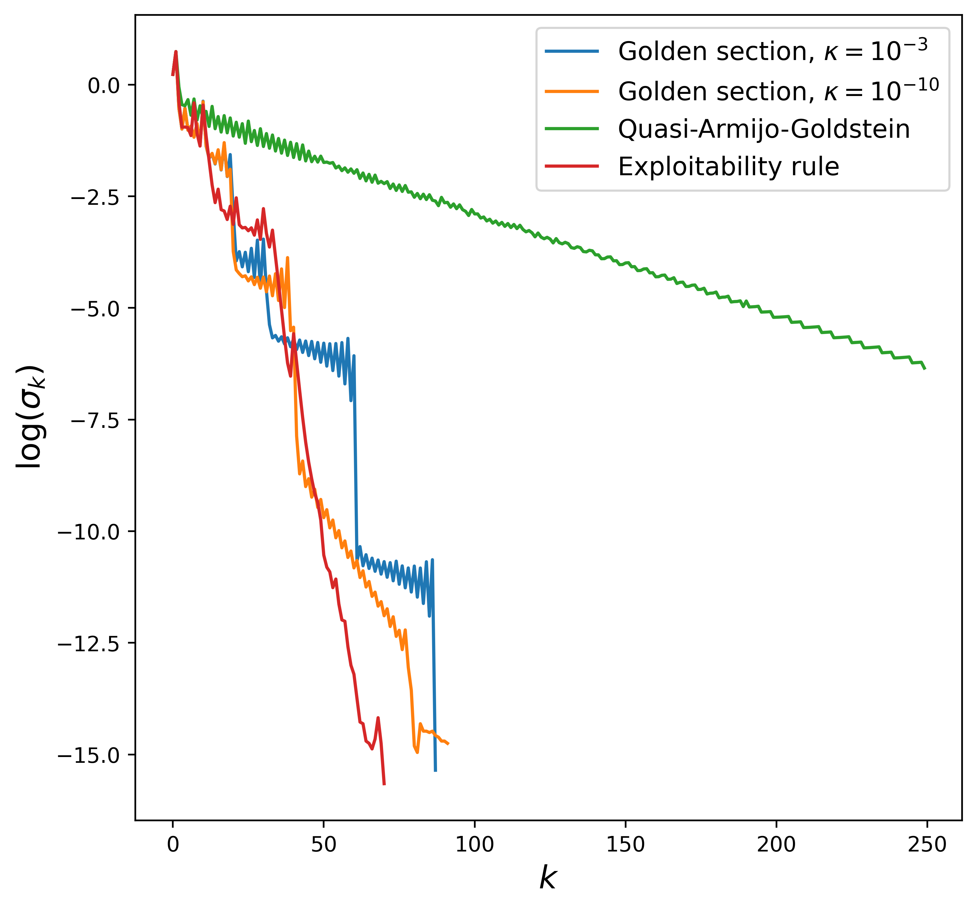
Figure 3: Convergence results for prescribed and adaptative stepsizes.
Refer to caption
(a) Logarithm of the exploitability for δk=p/(k+p)\delta_{k}=p/(k+p).
Refer to caption
(b) Log-log scale of the exploitablity for δk=p/(k+p)\delta_{k}=p/(k+p).
Refer to caption
(c) Logarithm of the exploitability for the prescribed stepsizes δk=(k+1)−α\delta_{k}=(k+1)^{-\alpha}.
Refer to caption
(d) Logarithm of the exploitability for the adaptative stepsizes.
Refer to caption
(e) Golden section search, QAG and exploitability-based stepsizes.

The convergence results are reported on Figure 3, for a maximal number N=250N=250 of iterations. We use the exploitability as an indicator of convergence, since it can be evaluated explicitely at each iteration. We recall that εk≤σk≤C​εk\varepsilon_{k}\leq\sigma_{k}\leq C\varepsilon_{k}.

  • •

    Prescribed stepsizes, with δk=p/(k+p)\delta_{k}=p/(k+p) and p∈{1,2,5,10}p\in\{1,2,5,10\}. Figures 3(a) and 3(b) show that the convergence of the exploitability with an empirical rate of convergence of order k−pk^{-p}, in accordance with Lemma 10. The value of pp which yields the best convergence, for a fixed number of iterations kk, increases slowly with respect to kk, in accordance with Remark 11.

  • •

    Prescribed stepsizes, with δk=(k+1)−α\delta_{k}=(k+1)^{-\alpha}, with α∈{0.6,0.7,0.8,0.9}\alpha\in\{0.6,0.7,0.8,0.9\}. See Figure 3(c). Similar comments can be done: a better asymptotic rate of convergence is observed for smaller values of α\alpha; the value of α\alpha which yields the best convergence for a fixed number of iterations kk, decreases with respect to kk. We have done some tests with smaller values of α\alpha, which are not shown on the figure. For N=250N=250 iterations, the performance is severely degraded for such values of α\alpha and convergence cannot be observed in a reasonable number of iterations.

  • •

    Adaptive stepsizes. See Figure 3(d). Optimal stepsizes are approximated with golden section search (see page 20) with tolerances κ=10−3\kappa=10^{-3} and κ=10−10\kappa=10^{-10}. The QAG condition is implemented with c=1/4c=1/4 and τ=0.9\tau=0.9. The choice of cc and τ\tau is here arbitrary since there is no general rule for the choice of these parameters (see [31, Chapter 3] for further discussions on the topic). The three methods all yield a linear convergence; the golden section and the exploitability-based methods are particularly fast. Note that in the case of optimal stepsizes, a very precise resolution of problem (14) with tolerance 10−1010^{-10} does not improve the convergence of the method, in comparison with the tolerance 10−310^{-3}.

Finally we compare the time required for the GCG algorithm to satisfy a precision criterion (σk≤10−3\sigma_{k}\leq 10^{-3} and σk≤10−4\sigma_{k}\leq 10^{-4}) for different stepsizes. For the considered example, the time needed to compute the adaptive stepsizes is not significantly longer than the time needed for the resolution of the HJB and the Fokker-Planck equation. Unsurprisingly, the adaptive stepsizes are more efficient than the tested prescribed stepsizes, for the two stopping criteria.

Learning method σk≤10−3\sigma_{k}\leq 10^{-3} σk≤10−4\sigma_{k}\leq 10^{-4}
Prescribed
δk=pk+p\delta_{k}=\frac{p}{k+p} p=1p=1 345.82345.82 3379.413379.41
p=2p=2 27.3927.39 85.2785.27
p=5p=5 11.1411.14 17.017.0
p=10p=10 13.9313.93 15.6115.61
δk=(k+1)−α\delta_{k}=(k+1)^{-\alpha} α=0.9\alpha=0.9 42.4642.46 132.37132.37
α=0.8\alpha=0.8 15.6215.62 32.332.3
α=0.7\alpha=0.7 9.469.46 14.9514.95
α=0.6\alpha=0.6 10.310.3 12.412.4
Adaptative
Quasi-Armijo-Goldstein 9.19.1 13.1113.11
Golden-section κ=10−3\kappa=10^{-3} 2.02.0 2.22.2
Golden-section κ=10−10\kappa=10^{-10} 2.542.54 2.682.68
Exploitability-based 3.263.26 3.913.91
Figure 4: Execution time in seconds of the generalized conditional gradient

5 Stability and convergence results

This section is dedicated to the analysis of Algorithm 1 and is organized in four subsections. We state in Subsection 5.1 some technical results concerning the well-posedness of the auxiliary mappings introduced in Subsection 2.3. Subsection 5.2 establishes a stability result (Proposition 21), necessary to prove the linear speed of convergence. Subsection 5.3 adresses the well-posedness of Algorithm 1 and the proof of Theorem 7. Subsection 5.4 is dedicated to the proof of Theorem 8.

5.1 Well-posedness of the auxiliary mappings

We provide here technical results, whose proofs can be found in the Appendix. We recall that the sets Θ\Theta, Ξ\Xi, and ΞR\Xi_{R} have been introduced in (3), (4), and (5).

Lemma 13.

Let R>0R>0. Let v∈Θv\in\Theta{} be such that ‖v‖Θ≤R\|v\|_{\Theta{}}\leq R Then 𝐌⁡[v]\bm{M}[v] is uniquely defined and lies in W2,1,q​(Q)W^{2,1,q}(Q). Moreover, there exists a constant C⁡(R)>0C(R)>0, independent of vv, such that ‖𝐌⁡[v]‖W2,1,q​(Q)≤C⁡(R)\|\bm{M}[v]\|_{W^{2,1,q}(Q)}\leq C(R). Finally, 𝐌​[v]​(x,t)≥0\bm{M}[v](x,t)\geq 0, for all (x,t)∈Q(x,t)\in Q.

Lemma 14.

Let R>0R>0. Let v1v_{1} and v2∈Θv_{2}\in\Theta{}. Let mi=𝐌⁡[vi]∈W2,1,q​(Q)m_{i}=\bm{M}[v_{i}]\in W^{2,1,q}(Q) for i∈{1,2}i\in\{1,2\}. Assume that ‖v1‖Θ≤R\|v_{1}\|_{\Theta{}}\leq R and ‖m2‖L∞​(Q)≤R\|m_{2}\|_{L^{\infty}(Q)}\leq R. Then, there exists a constant C⁡(R)C(R), independent of v1v_{1} and v2v_{2}, such that

‖m2−m1‖L∞​(0,T,L2​(𝕋d))≤C⁡(R)​(∫Q|v2−v1|2​m2​𝑑x​𝑑t)1/2.\|m_{2}-m_{1}\|_{L^{\infty}(0,T;L^{2}(\mathbb{T}^{d}))}\leq C(R)\Big(\int_{Q}|v_{2}-v_{1}|^{2}m_{2}\,\mathrm{d}x\,\mathrm{d}t\Big)^{1/2}.
Lemma 15.

Let R>0R>0. There exists a constant C⁡(R)C(R) such that for all (γ1,P1)(\gamma_{1},P_{1}) and (γ2,P2)(\gamma_{2},P_{2}) in ΞR\Xi_{R}, the following holds:

‖𝒖⁡[γ2,P2]−𝒖⁡[γ1,P1]‖L∞​(Q)≤C⁡(R)​(‖P2−P1‖L2​(0,T,ℝk)+‖γ2−γ1‖L∞​(Q)).\|\bm{u}[\gamma_{2},P_{2}]-\bm{u}[\gamma_{1},P_{1}]\|_{L^{\infty}(Q)}\leq C(R)\Big(\|P_{2}-P_{1}\|_{L^{2}(0,T;\mathbb{R}^{k})}+\|\gamma_{2}-\gamma_{1}\|_{L^{\infty}(Q)}\Big).
Proposition 16.

The map 𝐮\bm{u} is well-defined from Ξ\Xi to W2,1,q​(Q)W^{2,1,q}(Q). Moreover, for any R>0R>0, there exists a constant C⁡(R)>0C(R)>0 such that for any (γ,P)∈ΞR(\gamma,P)\in\Xi_{R}, ‖𝐮⁡[γ,P]‖W2,1,q​(Q)≤C⁡(R).\|\bm{u}[\gamma,P]\|_{W^{2,1,q}(Q)}\leq C(R).

Lemma 17.

The maps 𝐯\bm{v}, 𝐦\bm{m}, and 𝐰\bm{w} are well-defined from Ξ\Xi to Θ\Theta{}, W2,1,q​(Q)W^{2,1,q}(Q), and Θ\Theta{}, respectively. Moreover, for any R>0R>0, there exists C⁡(R)>0C(R)>0 such that for any (γ,P)∈ΞR(\gamma,P)\in\Xi_{R}, it holds:

‖𝒗⁡[γ,P]‖Θ+‖𝒎⁡[γ,P]‖W2,1,q​(Q)+‖𝒘⁡[γ,P]‖Θ≤C⁡(R).\|\bm{v}[\gamma,P]\|_{\Theta{}}+\|\bm{m}[\gamma,P]\|_{W^{2,1,q}(Q)}+\|\bm{w}[\gamma,P]\|_{\Theta{}}\leq C(R).
Lemma 18.

The mappings 𝛄\bm{\gamma} and 𝐏\bm{P} are well-defined. There exists a constant C>0C>0 such that for all m∈W2,1,q​(Q)m\in W^{2,1,q}(Q) and for all w∈Θw\in\Theta{},

‖γ‖W1,0,∞​(Q)+‖P‖L∞​(0,T,ℝk)≤C,\|\gamma\|_{W^{1,0,\infty}(Q)}+\|P\|_{L^{\infty}(0,T;\mathbb{R}^{k})}\leq C,

where γ=𝛄⁡[m]\gamma=\bm{\gamma}[m] and P=𝐏⁡[w]P=\bm{P}[w]. There exists a constant C>0C>0 such that for all m1m_{1} and m2m_{2} in W2,1,q​(Q)W^{2,1,q}(Q) and for all w1w_{1} and w2w_{2} in Θ\Theta{},

‖𝜸⁡[m2]−𝜸⁡[m1]‖L∞​(Q)≤\displaystyle\|\bm{\gamma}[m_{2}]-\bm{\gamma}[m_{1}]\|_{L^{\infty}(Q)}\leq{} C​‖m2−m1‖L∞​(0,T,L2​(𝕋d)),\displaystyle C\|m_{2}-m_{1}\|_{L^{\infty}(0,T;L^{2}(\mathbb{T}^{d}))},
‖𝑷⁡[w2]−𝑷⁡[w1]‖L2​(0,T,ℝk)≤\displaystyle\|\bm{P}[w_{2}]-\bm{P}[w_{1}]\|_{L^{2}(0,T;\mathbb{R}^{k})}\leq{} C​‖w2−w1‖L2​(Q,ℝd).\displaystyle C\|w_{2}-w_{1}\|_{L^{2}(Q;\mathbb{R}^{d})}.

5.2 Stability results for stochastic optimal control problems

The main result of this section, Proposition 21 and its Corollary 22, shows that any approximate solution to Problem ( P [ γ , P ] ) is close to its solution, for suitable norms. This is a key result for achieving linear convergence in the GCG method.

Lemma 19.

Let (γ^,P^)∈Ξ(\hat{\gamma},\hat{P})\in\Xi{}. Let m^=𝐦⁡[γ^,P^]\hat{m}=\bm{m}[\hat{\gamma},\hat{P}], v^=𝐯⁡[γ^,P^]\hat{v}=\bm{v}[\hat{\gamma},\hat{P}] and let w^=𝐰⁡[γ^,P^]\hat{w}=\bm{w}[\hat{\gamma},\hat{P}]. There exists a constant C>0C>0 such that for any (m,w)∈ℛ(m,w)\in\mathcal{R}, the following holds:

𝒵⁡[γ^,P^]​(m,w)−𝒵⁡[γ^,P^]​(m^,w^)≥1C​∫Q|v⁡(x,t)−v^​(x,t)|2​m​(x,t)​𝑑x​𝑑t,\mathcal{Z}[\hat{\gamma},\hat{P}](m,w)-\mathcal{Z}[\hat{\gamma},\hat{P}](\hat{m},\hat{w})\geq\frac{1}{C}\int_{Q}|v(x,t)-\hat{v}(x,t)|^{2}m(x,t)\,\mathrm{d}x\,\mathrm{d}t,

where v∈L∞​(Q,ℝd)v\in L^{\infty}(Q;\mathbb{R}^{d}) is such that w=m​vw=mv.

The proof of Lemma 19 relies on the following inequality.

Lemma 20.

Let (x,t)∈Q(x,t)\in Q. Let v∈ℝdv\in\mathbb{R}^{d}, p^∈ℝd\hat{p}\in\mathbb{R}^{d}, m≥0m\geq 0, and m^≥0\hat{m}\geq 0. Let v^=−Hp​(x,t,p^)\hat{v}=-H_{p}(x,t,\hat{p}). Let C>0C>0 be such that L(x,t,⋅)L(x,t,\cdot) is strongly convex with modulus 1/C1/C. Then,

L⁡(x,t,v)​m−L⁡(x,t,v^)​m^≥−H⁡(x,t,p)​(m−m^)−⟨p^,w−w^⟩+1C​|v−v^|2​m.L(x,t,v)m-L(x,t,\hat{v})\hat{m}\geq-H(x,t,p)(m-\hat{m})-\langle\hat{p},w-\hat{w}\rangle+\frac{1}{C}|v-\hat{v}|^{2}m.
Proof.

See [5, Proof of Proposition 2]. ∎

Proof of Lemma 19.

Using the definition of 𝒵⁡[γ^,P^]\mathcal{Z}[\hat{\gamma},\hat{P}], we have

𝒵⁡[γ^,P^]​(m,w)−𝒵⁡[γ^,P^]​(m^,w^)=∫Q(L⁡[v]​m−L⁡[v^]​m^)​𝑑x​𝑑t\displaystyle\mathcal{Z}[\hat{\gamma},\hat{P}](m,w)-\mathcal{Z}[\hat{\gamma},\hat{P}](\hat{m},\hat{w})=\int_{Q}\big(L[v]m-L[\hat{v}]\hat{m}\big)\,\mathrm{d}x\,\mathrm{d}t
+∫Qγ^(m−m^)dxdt+∫Q⟨A∗P,w−w^⟩dxdt+∫𝕋dg(m(T)−m^(T))dx.\displaystyle\qquad+\int_{Q}\hat{\gamma}(m-\hat{m})\,\mathrm{d}x\,\mathrm{d}t+\int_{Q}\langle A^{*}P,w-\hat{w}\rangle\,\mathrm{d}x\,\mathrm{d}t+\int_{\mathbb{T}^{d}}g(m(T)-\hat{m}(T))\,\mathrm{d}x. (21)

We set u^=𝒖⁡[γ^,P^]\hat{u}=\bm{u}[\hat{\gamma},\hat{P}]. By definition of v^\hat{v}, we have v^=−𝑯p​[∇u^+A⋆​P^]\hat{v}=-\bm{H}_{p}[\nabla\hat{u}+A^{\star}\hat{P}]. Applying Lemma 20 with p^=∇u^+A∗​P^\hat{p}=\nabla\hat{u}+A^{*}\hat{P}, we obtain

∫Q(L[v]m−L[v^]m^)dxdt≥−∫QH[∇u^+A∗P^](m−m¯)dxdt\displaystyle\int_{Q}\big(L[v]m-L[\hat{v}]\hat{m}\big)\,\mathrm{d}x\,\mathrm{d}t\geq-\int_{Q}H[\nabla\hat{u}+A^{*}\hat{P}](m-\bar{m})\,\mathrm{d}x\,\mathrm{d}t
−∫Q⟨∇u^+A∗P^,w−w¯⟩dxdt+1C∫Q|v−v^|2mdxdt.\displaystyle\qquad\quad-\int_{Q}\langle\nabla\hat{u}+A^{*}\hat{P},w-\bar{w}\rangle\,\mathrm{d}x\,\mathrm{d}t+\frac{1}{C}\int_{Q}|v-\hat{v}|^{2}m\,\mathrm{d}x\,\mathrm{d}t.

We inject the obtained inequality into (21) and we use 𝑯[∇u^+A∗P^]+γ^=−∂tu^−Δu^\bm{H}[\nabla\hat{u}+A^{*}\hat{P}]+\hat{\gamma}=-\partial_{t}\hat{u}-\Delta\hat{u}. This yields

𝒵[γ^,P^](m,w)−𝒵[γ^,P^](m^,w^)≥∫Q(−∂tu^−Δu^)(m−m^)dxdt\displaystyle\mathcal{Z}[\hat{\gamma},\hat{P}](m,w)-\mathcal{Z}[\hat{\gamma},\hat{P}](\hat{m},\hat{w})\geq\int_{Q}\big(-\partial_{t}\hat{u}-\Delta\hat{u}\big)\big(m-\hat{m}\big)\,\mathrm{d}x\,\mathrm{d}t
+∫Q⟨−∇u^,w−w^⟩dxdt+∫𝕋dg(m(T)−m^(T))dx+1C∫Q|v−v^|2mdxdt.\displaystyle\quad+\int_{Q}\langle-\nabla\hat{u},w-\hat{w}\rangle\,\mathrm{d}x\,\mathrm{d}t+\int_{\mathbb{T}^{d}}g(m(T)-\hat{m}(T))\,\mathrm{d}x+\frac{1}{C}\int_{Q}|v-\hat{v}|^{2}m\,\mathrm{d}x\,\mathrm{d}t.

The first three integrals in the right-hand side cancel out: this can be shown by doing an integration by parts and by using the Fokker-Planck equation satisfied by mm and m^\hat{m}. This concludes the proof. ∎

Proposition 21.

Let R>0R>0 and let (γ^,P^)∈ΞR(\hat{\gamma},\hat{P})\in\Xi_{R}. Let m^=𝐦⁡[γ^,P^]\hat{m}=\bm{m}[\hat{\gamma},\hat{P}] and let w^=𝐰⁡[γ^,P^]\hat{w}=\bm{w}[\hat{\gamma},\hat{P}]. Let (m,w)∈ℛ(m,w)\in\mathcal{R} be such that ‖m‖L∞​(Q)≤R\|m\|_{L^{\infty}(Q)}\leq R. There exists a constant C⁡(R)C(R) such that for any (m,w)∈ℛ(m,w)\in\mathcal{R},

‖m−m^‖L∞​(0,T,L2​(𝕋d))≤\displaystyle\|m-\hat{m}\|_{L^{\infty}(0,T;L^{2}(\mathbb{T}^{d}))}\leq{} C⁡(R)​σ,\displaystyle C(R)\sqrt{\sigma},
‖w−w^‖L2​(Q,ℝd)≤\displaystyle\|w-\hat{w}\|_{L^{2}(Q;\mathbb{R}^{d})}\leq{} C​(R)​(σ+σ),\displaystyle C(R)(\sqrt{\sigma}+\sigma),

where σ=𝒵⁡[γ^,P^]​(m,w)−𝒵⁡[γ^,P^]​(m^,w^)\sigma=\mathcal{Z}[\hat{\gamma},\hat{P}](m,w)-\mathcal{Z}[\hat{\gamma},\hat{P}](\hat{m},\hat{w}).

As a consequence of Proposition 21, (𝒎⁡[γ^,P^],𝒘⁡[γ^,P^])(\bm{m}[\hat{\gamma},\hat{P}],\bm{w}[\hat{\gamma},\hat{P}]) is the unique solution to Problem ( P [ γ , P ] ), with (γ,P)=(γ^,P^)(\gamma,P)=(\hat{\gamma},\hat{P}).

Proof of Proposition 21.

Lemma 20 yields ∫Q|v−v^|2​m​𝑑x​𝑑t≤C​σ\int_{Q}|v-\hat{v}|^{2}m\,\mathrm{d}x\,\mathrm{d}t\leq C\sigma. By Lemma 17, we know that ‖v^‖W1,0,∞​(Q,ℝd)≤C\|\hat{v}\|_{W^{1,0,\infty}(Q;\mathbb{R}^{d})}\leq C, for some constant depending on RR. Applying next Lemma 14, we obtain the estimate of ‖m−m^‖L∞​(0,T,L2​(𝕋d))\|m-\hat{m}\|_{L^{\infty}(0,T;L^{2}(\mathbb{T}^{d}))}. The estimate of ‖w−w^‖L2​(Q,ℝd)\|w-\hat{w}\|_{L^{2}(Q;\mathbb{R}^{d})} follows directly from w−w^=m⁡(v−v^)+(m−m^)​v^.w-\hat{w}=m(v-\hat{v})+(m-\hat{m})\hat{v}. The proposition is proved. ∎

Corollary 22.

Let R>0R>0. Let (m,w)∈ℛ(m,w)\in\mathcal{R} be such that ‖m‖L∞​(Q)≤R\|m\|_{L^{\infty}(Q)}\leq R. There exists a constant C⁡(R)C(R) such that

‖m−m¯‖L∞​(0,T,L2​(𝕋d))≤\displaystyle\|m-\bar{m}\|_{L^{\infty}(0,T;L^{2}(\mathbb{T}^{d}))}\leq{} C⁡(R)​ε\displaystyle C(R)\sqrt{\varepsilon}
‖w−w¯‖L2​(Q,ℝd)≤\displaystyle\|w-\bar{w}\|_{L^{2}(Q;\mathbb{R}^{d})}\leq{} C​(R)​(ε+ε),\displaystyle C(R)(\sqrt{\varepsilon}+\varepsilon),

where ε=𝒥⁡(m,w)−𝒥⁡(m¯,w¯)\varepsilon=\mathcal{J}(m,w)-\mathcal{J}(\bar{m},\bar{w}).

Proof.

By definition, m¯=𝒎⁡[γ¯,P¯]\bar{m}=\bm{m}[\bar{\gamma},\bar{P}] and w¯=𝒘⁡[γ¯,P¯]\bar{w}=\bm{w}[\bar{\gamma},\bar{P}]. We obtain the announced estimates by combining Corollary 25 and Proposition 21. ∎

5.3 Well-posedness of Algorithm 1 and proof of Theorem 7.

In this subsection the well-posedness of Algorithm 1 is established. The proof of Theorem 7 is a direct consequence of the well-posedness and the stability results established in the previous subsection.

Proposition 23.

Algorithm 1 generates sequences in the following sets: (m¯k,w¯k)∈ℛ(\bar{m}_{k},\bar{w}_{k})\in\mathcal{R}, (γk,Pk)∈Ξ(\gamma_{k},P_{k})\in\Xi{}, (uk,vk)∈W2,1,q​(Q)×Θ(u_{k},v_{k})\in W^{2,1,q}(Q)\times\Theta, (mk,wk)∈ℛ(m_{k},w_{k})\in\mathcal{R}, for all k∈ℕk\in\mathbb{N}. Moreover, there exists a constant C>0C>0 such that (γk,Pk)∈ΞC(\gamma_{k},P_{k})\in\Xi{}_{C} and such that

‖uk‖W2,1,q​(Q)+‖vk‖Θ≤\displaystyle\|u_{k}\|_{W^{2,1,q}(Q)}+\|v_{k}\|_{\Theta{}}\leq{} C,\displaystyle C,
‖mk‖W2,1,q​(Q)+‖wk‖Θ≤\displaystyle\|m_{k}\|_{W^{2,1,q}(Q)}+\|w_{k}\|_{\Theta{}}\leq{} C,\displaystyle C,
‖m¯k‖W2,1,q​(Q)+‖w¯k‖Θ≤\displaystyle\|\bar{m}_{k}\|_{W^{2,1,q}(Q)}+\|\bar{w}_{k}\|_{\Theta{}}\leq{} C,\displaystyle C,

for all k∈ℕk\in\mathbb{N}. Finally, there exists a constant C>0C>0 such that εk≤C\varepsilon_{k}\leq C, for all k∈ℕk\in\mathbb{N}.

Proof.

The well-posedness of the algorithm m¯k\bar{m}_{k}, w¯k\bar{w}_{k}, γk\gamma_{k}, PkP_{k}, uku_{k}, vkv_{k}, mkm_{k}, and wkw_{k} can easily be established by induction. Lemma 18 shows the existence of a constant C0C_{0}, independent of kk such that (γk,Pk)∈ΞC0(\gamma_{k},P_{k})\in\Xi_{C_{0}}, for any k∈ℕk\in\mathbb{N}. Applying next Proposition 16 and Lemma 17 with R=C0R=C_{0}, we deduce that ‖uk‖W2,1,q​(Q)+‖vk‖Θ≤C\|u_{k}\|_{W^{2,1,q}(Q)}+\|v_{k}\|_{\Theta{}}\leq C and ‖mk‖W2,1,q​(Q)+‖wk‖Θ≤C\|m_{k}\|_{W^{2,1,q}(Q)}+\|w_{k}\|_{\Theta{}}\leq C, for some constant CC independent of kk. The inequality ‖m¯k‖W2,1,q​(Q)+‖w¯k‖Θ≤C\|\bar{m}_{k}\|_{W^{2,1,q}(Q)}+\|\bar{w}_{k}\|_{\Theta{}}\leq C follows then immediately from the triangle inequality. Using the convexity of ℛ\mathcal{R} given in Lemma 5, we deduce by induction that (m¯k,w¯k)∈ℛ(\bar{m}_{k},\bar{w}_{k})\in\mathcal{R}, for all k∈ℕk\in\mathbb{N}. The bounds on mkm_{k} and vkv_{k} imply the existence of a constant CC such 𝒥⁡(mk,wk)≤C\mathcal{J}(m_{k},w_{k})\leq C, since

𝒥⁡(mk,wk)=∫Q𝑳⁡[vk]​mk​𝑑x​𝑑t+∫0T(𝑭⁡[mk]+𝚽⁡[A⁡(mk​vk)])​𝑑t+∫𝕋dg​mk​(T)​𝑑x.\mathcal{J}(m_{k},w_{k})=\int_{Q}\bm{L}[v_{k}]m_{k}\,\mathrm{d}x\,\mathrm{d}t+\int_{0}^{T}\big(\bm{F}[m_{k}]+\bm{\Phi}[A(m_{k}v_{k})]\big)\mathrm{d}t+\int_{\mathbb{T}^{d}}gm_{k}(T)\,\mathrm{d}x.

The boundedness of 𝒥⁡(m¯k,w¯k)\mathcal{J}(\bar{m}_{k},\bar{w}_{k}) follows then by induction, since 𝒥\mathcal{J} is convex and thus

𝒥⁡(m¯k+1,w¯k+1)≤(1−δk)​𝒥​(m¯k,w¯k)+δk​𝒥​(mk,wk).\mathcal{J}(\bar{m}_{k+1},\bar{w}_{k+1})\leq(1-\delta_{k})\mathcal{J}(\bar{m}_{k},\bar{w}_{k})+\delta_{k}\mathcal{J}(m_{k},w_{k}).

The proposition is proved. ∎

Proof of Theorem 7

The first estimate concerning ‖m¯k−m¯‖L∞​(0,T,L2​(𝕋d))\|\bar{m}_{k}-\bar{m}\|_{L^{\infty}(0,T;L^{2}(\mathbb{T}^{d}))} and ‖w¯k−w¯‖L2​(Q,ℝd)\|\bar{w}_{k}-\bar{w}\|_{L^{2}(Q;\mathbb{R}^{d})} is obtained by combining Corollary 22, the boundedness of εk\varepsilon_{k}, and the boundedness of ‖mk‖L∞​(Q)\|m_{k}\|_{L^{\infty}(Q)}. The second estimate on ‖γk−γ¯‖L∞​(Q)\|\gamma_{k}-\bar{\gamma}\|_{L^{\infty}(Q)} and ‖Pk−P¯‖L∞​(0,T,ℝk)\|P_{k}-\bar{P}\|_{L^{\infty}(0,T;\mathbb{R}^{k})} is obtained by combining the first estimate and Lemma 18. The third estimate on ‖uk−u¯‖L∞​(Q)\|u_{k}-\bar{u}\|_{L^{\infty}(Q)} follows from the second one and from Lemma 15. Using Proposition 23 and Lemma 1, there exists C>0C>0 such that (γk,Pk)∈ΞC(\gamma_{k},P_{k})\in\Xi{}_{C} and ‖m¯k‖L∞​(Q)≤C\|\bar{m}_{k}\|_{L^{\infty}(Q)}\leq C, for all k∈ℕk\in\mathbb{N}. Moreover, by construction, mk=𝒎⁡[γk,Pk]m_{k}=\bm{m}[\gamma_{k},P_{k}] and wk=𝒘⁡[γk,Pk]w_{k}=\bm{w}[\gamma_{k},P_{k}] and the pair (m¯k,w¯k)(\bar{m}_{k},\bar{w}_{k}) is σk\sigma_{k}-optimal for the minimization problem of 𝒵⁡[γk,Pk]​(⋅)\mathcal{Z}[\gamma_{k},P_{k}](\cdot). Therefore, Proposition 21 applies and yields the last estimate that was to be proved.

5.4 Proof of Theorem 8

In this subsection we prove Theorem 8, leveraging techniques from [26].

Lemma 24.

Let (m1,w1)(m_{1},w_{1}) and (m2,w2)(m_{2},w_{2}) be in ℛ\mathcal{R}. Let γ1=𝛄⁡[m1]\gamma_{1}=\bm{\gamma}[m_{1}] and let P1=𝐏⁡[w1]P_{1}=\bm{P}[w_{1}]. Then, there exists a constant C>0C>0, independent of (m1,w1)(m_{1},w_{1}) and (m2,w2)(m_{2},w_{2}) such that

∫Qγ1​(m2−m1)​𝑑x​𝑑t+∫0T⟨A⁡[w2−w1],P1⟩​𝑑t≤𝒥2​(m2,w2)−𝒥2​(m1,w1)\int_{Q}\gamma_{1}(m_{2}-m_{1})\,\mathrm{d}x\,\mathrm{d}t+\int_{0}^{T}\langle A[w_{2}-w_{1}],P_{1}\rangle\,\mathrm{d}t\leq\mathcal{J}_{2}(m_{2},w_{2})-\mathcal{J}_{2}(m_{1},w_{1}) (22)

and

𝒥2​(m2,w2)−𝒥2​(m1,w1)≤∫Qγ1​(m2−m1)​𝑑x​𝑑t+∫0T⟨A⁡[w2−w1],P1⟩​𝑑t\displaystyle\mathcal{J}_{2}(m_{2},w_{2})-\mathcal{J}_{2}(m_{1},w_{1})\leq\int_{Q}\gamma_{1}(m_{2}-m_{1})\,\mathrm{d}x\,\mathrm{d}t+\int_{0}^{T}\langle A[w_{2}-w_{1}],P_{1}\rangle\,\mathrm{d}t
+C1∫0T∥m2(t,⋅)−m1(t,⋅)∥L2​(𝕋d)∥m2(t,⋅)−m1(t,⋅)∥L1​(𝕋d)dt\displaystyle\qquad+C_{1}\int_{0}^{T}\|m_{2}(t,\cdot)-m_{1}(t,\cdot)\|_{L^{2}(\mathbb{T}^{d})}\|m_{2}(t,\cdot)-m_{1}(t,\cdot)\|_{L^{1}(\mathbb{T}^{d})}\,\mathrm{d}t
+C2∫0T|∫𝕋da(x,t)(w2(x,t)−w1(x,t))dx|2dt.\displaystyle\qquad+C_{2}\int_{0}^{T}\Big|\int_{\mathbb{T}^{d}}a(x,t)(w_{2}(x,t)-w_{1}(x,t))\,\mathrm{d}x\Big|^{2}\,\mathrm{d}t. (23)
Proof.

Using the definitions of γ1\gamma_{1} and P1P_{1}, we obtain

(𝒥2​(m2,w2)−𝒥2​(m1,w1))−(∫Qγ1​(m2−m1)​𝑑x​𝑑t+∫0T⟨A⁡[w2−w1],P1⟩​𝑑t)\displaystyle\big(\mathcal{J}_{2}(m_{2},w_{2})-\mathcal{J}_{2}(m_{1},w_{1})\big)-\Big(\int_{Q}\gamma_{1}(m_{2}-m_{1})\,\mathrm{d}x\,\mathrm{d}t+\int_{0}^{T}\langle A[w_{2}-w_{1}],P_{1}\rangle\,\mathrm{d}t\Big)
=(a)+(b),\displaystyle\qquad=(a)+(b),

where

(a)\displaystyle(a){} =∫0T(𝑭⁡[m2]​(t)−𝑭⁡[m1]​(t)−∫𝕋df⁡[m1]​(x,t)​(m2​(x,t)−m1​(x,t))​𝑑x)​𝑑t,\displaystyle=\int_{0}^{T}\Big(\bm{F}[m_{2}](t)-\bm{F}[m_{1}](t)-\int_{\mathbb{T}^{d}}f[m_{1}](x,t)\big(m_{2}(x,t)-m_{1}(x,t)\big)\,\mathrm{d}x\Big)\,\mathrm{d}t,
(b)\displaystyle(b){} =∫0T(𝚽⁡[A​w2]−𝚽⁡[A​w1]−⟨ϕ⁡[A​w1]​(t),A​w2​(t)−A​w1​(t)⟩)​𝑑t.\displaystyle=\int_{0}^{T}\big(\bm{\Phi}[Aw_{2}]-\bm{\Phi}[Aw_{1}]-\langle\bm{\phi}[Aw_{1}](t),Aw_{2}(t)-Aw_{1}(t)\rangle\big)\,\mathrm{d}t.

Using Assumption (H6), we obtain that

(a)=\displaystyle(a)={} ∫0T∫01∫𝕋d(f⁡[m1+s⁡(m2−m1)]−f⁡[m1])​(m2−m1)​𝑑x​𝑑s​𝑑t.\displaystyle\int_{0}^{T}\int_{0}^{1}\int_{\mathbb{T}^{d}}\big(f[m_{1}+s(m_{2}-m_{1})]-f[m_{1}]\big)(m_{2}-m_{1})\,\mathrm{d}x\,\mathrm{d}s\,\mathrm{d}t.

Then Assumptions (H5) and (H6) imply that

0≤(a)≤C1​∫0T‖m2​(t,⋅)−m1​(t,⋅)‖L2​(𝕋d)​‖m2​(t,⋅)−m1​(t,⋅)‖L1​(𝕋d)​𝑑t.0\leq(a)\leq C_{1}\int_{0}^{T}\|m_{2}(t,\cdot)-m_{1}(t,\cdot)\|_{L^{2}(\mathbb{T}^{d})}\|m_{2}(t,\cdot)-m_{1}(t,\cdot)\|_{L^{1}(\mathbb{T}^{d})}\,\mathrm{d}t.

We estimate (b)(b) in a similar way and obtain inequalities (22) and (23) easily. ∎

Corollary 25.

Let (m1,w1)(m_{1},w_{1}) and (m2,w2)(m_{2},w_{2}) be in ℛ\mathcal{R}. Let γ1=𝛄⁡[m1]\gamma_{1}=\bm{\gamma}[m_{1}] and let P1=𝐏⁡[w1]P_{1}=\bm{P}[w_{1}]. Then,

𝒵⁡[γ1,P1]​(m2,w2)−𝒵⁡[γ1,P1]​(m1,w1)≤𝒥⁡(m2,w2)−𝒥⁡(m1,w1).\mathcal{Z}[\gamma_{1},P_{1}](m_{2},w_{2})-\mathcal{Z}[\gamma_{1},P_{1}](m_{1},w_{1})\leq\mathcal{J}(m_{2},w_{2})-\mathcal{J}(m_{1},w_{1}).
Proof.

This is an immediate consequence of inequality (22) from Lemma 24 and the definitions of 𝒥\mathcal{J} and 𝒵\mathcal{Z}. ∎

Lemma 26.

For all k∈ℕk\in\mathbb{N}, it holds that εk≤σk\varepsilon_{k}\leq\sigma_{k}.

Proof.

By Corollary 25, we have for all (m,w)∈ℛ(m,w)\in\mathcal{R}

𝒵⁡[γk,Pk]​(m¯k,w¯k)−𝒵⁡[γk,Pk]​(m,w)≤𝒥⁡(m¯k,w¯k)−𝒥⁡(m,w)≤εk.\mathcal{Z}[\gamma_{k},P_{k}](\bar{m}_{k},\bar{w}_{k})-\mathcal{Z}[\gamma_{k},P_{k}](m,w)\leq\mathcal{J}(\bar{m}_{k},\bar{w}_{k})-\mathcal{J}(m,w)\\ \leq\varepsilon_{k}.

By definition, σk\sigma_{k} is the supremum of the left-hand side with respect to (m,w)(m,w). The conclusion follows immediately. ∎

Lemma 27.

Let C1>0C_{1}>0 and C2>0C_{2}>0 denote the Lipschitz constants of ff and ϕ\phi (see Assumption (H5)). Then for any δ∈[0,1]\delta\in[0,1], it holds that

𝒥⁡(m¯kδ,w¯kδ)≤𝒥⁡(m¯k,w¯k)−δ​σk+(C1​Dk(1)+C2​Dk(2))​δ2,\mathcal{J}(\bar{m}_{k}^{\delta},\bar{w}_{k}^{\delta})\leq\mathcal{J}(\bar{m}_{k},\bar{w}_{k})-\delta\sigma_{k}+\big(C_{1}D_{k}^{(1)}+C_{2}D_{k}^{(2)}\big)\delta^{2}, (24)

where (m¯kδ,w¯kδ)(\bar{m}_{k}^{\delta},\bar{w}_{k}^{\delta}) is defined by (12) and where Dk(1)D_{k}^{(1)} and Dk(2)D_{k}^{(2)} are defined by (• ‣ 3.2). Moreover, there exists a constant C>0C>0 such that

𝒥⁡(m¯kδ,w¯kδ)≤𝒥⁡(m¯k,w¯k)−δ​σk+C​σk​δk2.\mathcal{J}(\bar{m}_{k}^{\delta},\bar{w}_{k}^{\delta})\leq\mathcal{J}(\bar{m}_{k},\bar{w}_{k})-\delta\sigma_{k}+C\sigma_{k}\delta_{k}^{2}. (25)

Recall that the terms Dk(1)D_{k}^{(1)} and Dk(2)D_{k}^{(2)} represent the distance of the current approximate solution to the solution of the (partially) linearized problem. In the classical proof of convergence of the Frank-Wolfe algorithm, one writes a similar estimate to (24), where Dk(1)D_{k}^{(1)} and Dk(2)D_{k}^{(2)} are simply bounded by some constant. In order to achieve linear convergence (instead of the classical sublinear rate of convergence), it is crucial to keep these terms and to estimate them with the exploitability σk\sigma_{k}, as will become clear in the next section. This proof technique is largely inspired by [26, Section 4.3].

Proof of Lemma 27.

The proof relies on the decomposition 𝒥=𝒥1+𝒥2\mathcal{J}=\mathcal{J}_{1}+\mathcal{J}_{2} introduced in (1). First, by convexity of L~\tilde{L}, we have

𝒥1​(m¯kδ,w¯kδ)−𝒥1​(m¯k,w¯k)≤δ⁡(𝒥1​(mk,wk)−𝒥1​(m¯k,w¯k)).\mathcal{J}_{1}(\bar{m}_{k}^{\delta},\bar{w}_{k}^{\delta})-\mathcal{J}_{1}(\bar{m}_{k},\bar{w}_{k})\leq\delta\big(\mathcal{J}_{1}(m_{k},w_{k})-\mathcal{J}_{1}(\bar{m}_{k},\bar{w}_{k})\big). (26)

Next, using inequality (23) of Lemma 24, we obtain that

𝒥2​(m¯kδ,w¯kδ)−𝒥2​(m¯k,w¯k)≤δ​∫Qγk​(mk−m¯k)​𝑑x​𝑑t\displaystyle\mathcal{J}_{2}(\bar{m}_{k}^{\delta},\bar{w}_{k}^{\delta})-\mathcal{J}_{2}(\bar{m}_{k},\bar{w}_{k})\leq\delta\int_{Q}\gamma_{k}(m_{k}-\bar{m}_{k})\,\mathrm{d}x\,\mathrm{d}t
+δ∫0T⟨A[wk−w¯k],Pk⟩dt+Cδ2(∥mk−m¯k∥L2​(Q)2+∥wk−w¯k∥L2​(Q,ℝd)2).\displaystyle\quad+\delta\int_{0}^{T}\langle A[w_{k}-\bar{w}_{k}],P_{k}\rangle\,\mathrm{d}t+C\delta^{2}\Big(\|m_{k}-\bar{m}_{k}\|_{L^{2}(Q)}^{2}+\|w_{k}-\bar{w}_{k}\|_{L^{2}(Q;\mathbb{R}^{d})}^{2}\Big). (27)

By definition of 𝒵⁡[γk,Pk]\mathcal{Z}[\gamma_{k},P_{k}], we have

σk=\displaystyle\sigma_{k}={} 𝒵⁡[γk,Pk]​(m¯k,w¯k)−𝒵⁡[γk,Pk]​(mk,wk)\displaystyle\mathcal{Z}[\gamma_{k},P_{k}](\bar{m}_{k},\bar{w}_{k})-\mathcal{Z}[\gamma_{k},P_{k}](m_{k},w_{k})
=\displaystyle={} 𝒥1​(mk,wk)−𝒥1​(m¯k,w¯k)\displaystyle\mathcal{J}_{1}(m_{k},w_{k})-\mathcal{J}_{1}(\bar{m}_{k},\bar{w}_{k})
+∫Qγk(mk−m¯k)dxdt+∫0T⟨A[wk−w¯k],Pk⟩dt.\displaystyle\quad+\int_{Q}\gamma_{k}(m_{k}-\bar{m}_{k})\,\mathrm{d}x\,\mathrm{d}t+\int_{0}^{T}\langle A[w_{k}-\bar{w}_{k}],P_{k}\rangle\,\mathrm{d}t. (28)

Finally, by Theorem 7 we have

‖mk−m¯k‖L∞​(0,T,L2​(𝕋d))2+‖wk−w¯k‖L2​(Q,ℝd)2≤C​σk.\|m_{k}-\bar{m}_{k}\|_{L^{\infty}(0,T;L^{2}(\mathbb{T}^{d}))}^{2}+\|w_{k}-\bar{w}_{k}\|_{L^{2}(Q;\mathbb{R}^{d})}^{2}\leq C\sigma_{k}. (29)

Summing up (26) and (27) and combining the result with (28) and (29), we obtain the announced result. ∎

Lemma 28.

There exists C>0C>0 such that σk≤C​εk\sigma_{k}\leq C\varepsilon_{k}, for all k∈ℕk\in\mathbb{N}.

Proof.

For any δ∈[0,1]\delta\in[0,1], Lemma 27 yields 𝒥⁡(m¯,w¯)≤𝒥⁡(m¯k,w¯k)−δ​σk+C​δ2​σk\mathcal{J}(\bar{m},\bar{w})\leq\mathcal{J}(\bar{m}_{k},\bar{w}_{k})-\delta\sigma_{k}+C\delta^{2}\sigma_{k}. It follows that

0≤εk−(1−C​δ)​δ​σk.0\leq\varepsilon_{k}-(1-C\delta)\delta\sigma_{k}. (30)

Increasing if necessary the value of CC, we can assume that C≥1/2C\geq 1/2. Taking δ=1/(2​C)\delta=1/(2C), we conclude that 0≤ε−1/(4​C)​σk0\leq\varepsilon-1/(4C)\sigma_{k}, as was to be proved. ∎

Proof of Theorem 8

We start with the proof of the second part of the theorem, which is almost direct. Combining the upper bound of the cost function proved in Lemma 27 (inequality (25)) with the inequality εk≤σk\varepsilon_{k}\leq\sigma_{k} and the bound on the exploitability obtained in Lemma 28, we obtain the following inequality:

εj+1≤(1−δj+C​δj2)​εj,∀j∈ℕ.\varepsilon_{j+1}\leq\big(1-\delta_{j}+C\delta_{j}^{2}\big)\varepsilon_{j},\quad\forall j\in\mathbb{N}.

Here the constant CC is independent of the choice of stepsize. Multiplying the obtained inequalities for j=0,…,kj=0,\ldots,k, we obtain

εj+1≤ε0​exp⁡(∑j=0kln⁡(1−δj+C​δj2)).\varepsilon_{j+1}\leq\varepsilon_{0}\exp\Big(\sum_{j=0}^{k}\,\ln\left(1-\delta_{j}+C\delta_{j}^{2}\right)\Big).

Using next the inequality ln⁡(x)≤x−1\ln(x)\leq x-1, satisfied for any x>0x>0, we obtain the desired result, inequality (19).

Let us consider the case of adaptive stepsizes. Let us fix the iteration number kk. It suffices to show that for δk\delta_{k} satisfying either (14), (15), or (16), there exists a constant β∈(0,1)\beta\in(0,1), independent of kk, such that εk+1≤β​εk\varepsilon_{k+1}\leq\beta\varepsilon_{k}.

Case of the QAG condition. The main idea is to show that the QAG condition is satisfied when δ\delta is smaller than a certain threshold, which is independent of kk. Let δ>0\delta>0 be such that the condition is not satisfied. Then, using Lemma 27,

𝒥⁡(m¯,w¯)−c​δ​σk<𝒥⁡(m¯kδ,w¯kδ)≤𝒥⁡(m¯,w¯)−δ​σk+C​δ2​σk.\mathcal{J}(\bar{m},\bar{w})-c\delta\sigma_{k}<\mathcal{J}(\bar{m}_{k}^{\delta},\bar{w}_{k}^{\delta})\leq\mathcal{J}(\bar{m},\bar{w})-\delta\sigma_{k}+C\delta^{2}\sigma_{k}.

Re-arranging, we deduce that δ>δ¯:=(1−c)C>0\delta>\bar{\delta}:=\frac{(1-c)}{C}>0. By contraposition, the QAG condition holds true for any δ\delta such that δ≤δ¯\delta\leq\bar{\delta}.

We can now prove that iki_{k} is finite and uniformly bounded. Two cases can be considered. If δ¯≥1\bar{\delta}\geq 1, then ik=0i_{k}=0 and δk=1\delta_{k}=1. Otherwise, for any j∈ℕj\in\mathbb{N}, we have

τj≤δ¯⟺j≥ln⁡(δ¯)/ln⁡(τ).\tau^{j}\leq\bar{\delta}\Longleftrightarrow j\geq\mathrm{ln}(\bar{\delta})/\mathrm{ln}(\tau).

Therefore, ik≤⌈ln⁡(δ¯)/ln⁡(τ)⌉i_{k}\leq\lceil\mathrm{ln}(\bar{\delta})/\mathrm{ln}(\tau)\rceil. If ik=0i_{k}=0, then δk=1\delta_{k}=1. Otherwise, if ik>0i_{k}>0, then τik−1\tau^{i_{k}-1} does not satisfy the QAG condition and therefore, τik−i≥δ¯\tau^{i_{k}-i}\geq\bar{\delta} and thus δk=τik≥τ​δ¯\delta_{k}=\tau^{i_{k}}\geq\tau\bar{\delta}. So, in all cases, we have δk≥δmin:=min⁡(1,τ​δ¯)\delta_{k}\geq\delta_{\min}:=\min(1,\tau\bar{\delta}). It follows that

εk+1=\displaystyle\varepsilon_{k+1}={} 𝒥⁡(m¯k+1,w¯k+1)−𝒥⁡(m¯,w¯)\displaystyle\mathcal{J}(\bar{m}_{k+1},\bar{w}_{k+1})-\mathcal{J}(\bar{m},\bar{w})
≤\displaystyle\leq{} (𝒥⁡(m¯k,w¯k)−𝒥⁡(m¯,w¯))−c​σk​δk\displaystyle\big(\mathcal{J}(\bar{m}_{k},\bar{w}_{k})-\mathcal{J}(\bar{m},\bar{w})\big)-c\sigma_{k}\delta_{k}
≤\displaystyle\leq{} εk−c​δmin​σk≤(1−c​δmin)​εk.\displaystyle\varepsilon_{k}-c\delta_{\min}\sigma_{k}\leq(1-c\delta_{\min})\varepsilon_{k}. (31)

The last inequality was obtained with Lemma 26.

Case of exploitability-based stepsizes. Let us set ak=(C1​Dk(1)+C2​Dk(2))a_{k}=\big(C_{1}D_{k}^{(1)}+C_{2}D_{k}^{(2)}\big). By definition, δk=min⁡(1,σk2​ak)\delta_{k}=\min\big(1,\frac{\sigma_{k}}{2a_{k}}\big). Assume that σk≥2​ak\sigma_{k}\geq 2a_{k}, i.e. ak≤σk/2a_{k}\leq\sigma_{k}/2. Then δk=1\delta_{k}=1. Inequality (24) in Lemma 27 and Lemma 26 yield

εk+1≤εk−σk2≤12​εk.\varepsilon_{k+1}\leq\varepsilon_{k}-\frac{\sigma_{k}}{2}\leq\frac{1}{2}\varepsilon_{k}.

Now assume that σk<2​ak\sigma_{k}<2a_{k}. Then δk=σk2​ak\delta_{k}=\frac{\sigma_{k}}{2a_{k}}. By (24), εk+1≤εk−σk24​ak.\varepsilon_{k+1}\leq\varepsilon_{k}-\frac{\sigma_{k}^{2}}{4a_{k}}. It follows from the last estimate of Theorem 7 that ak≤C​σka_{k}\leq C\sigma_{k}. Therefore, by Lemma 26,

εk+1≤εk−σk4​C≤(1−14​C)​εk,\varepsilon_{k+1}\leq\varepsilon_{k}-\frac{\sigma_{k}}{4C}\leq\Big(1-\frac{1}{4C}\Big)\varepsilon_{k},

as was to be proved.

Case of an optimal stepsize. If δk\delta_{k} minimizes 𝒥⁡(m¯kδ,w¯kδ)\mathcal{J}(\bar{m}_{k}^{\delta},\bar{w}_{k}^{\delta}), then (31) is necessarily satisfied. This concludes the proof of the theorem.

6 Conclusion

The connection between the GCG method and fictitious play investigated in this article is not specific to second-order MFGs and could be established in different settings. Before discussing some possible extensions of our work, let us make some general comments.

  • •

    While we have focused here on a class of MFGs with a convex potential formulation, the case of nonconvex potential MFGs is also of interest. An example of interactions with a nonconvex variational structure, arising from a consensus model, is given in [33]. In this situation the GCG algorithm might not converge. In [22], the authors only show that any convergent sub-sequence generated by the fictitious play converges to an equilibrium. This problem can be tackled, assuming that solutions are stable [8]. Also very few results are available concerning the conditional gradient in the nonconvex setting. The article [27] shows that in the case of nonconvex optimization problems, the Frank-Wolfe algorithm converges to stationary points, when suitable stepsizes are utilized. The notion of stationarity involved in [27] should lead to the MFG system associated with the nonconvex potential formulation.

  • •

    The very first assumption to be satisfied in the analysis of the Frank-Wolfe algorithm is the Lipschitz continuity of the gradient of the cost function. In the case of MFGs, this means that the coupling functions should Lipschitz-continuous in suitable functional spaces. As a consequence, the analysis of the GCG method for potential MFGs with nonsmooth coupling functions (for example, MFGs with a local congestion term) may be particularly difficult.

  • •

    In general, the GCG method only has a sublinear rate of convergence. The linear rate of convergence obtained in this article heavily relies on the specific stability analysis which was done in Section 5.2 for optimal control problems.

A first natural extension of our work concerns the case of an unbounded domain. We expect that the linear convergence can be achieved. At a technical level, one difficulty concerns the boundedness of the distribution mkm_{k}. While we have established it with the help of parabolic estimates, we could follow the methodology of [15] to address this more general case. We also think that linear convergence of the GCG method can be established for fully discrete MFGs, as formulated in [6], taking Lipschitz-continuous coupling functions and a strongly convex running cost. Finally, we mention the case of first-order MFGs, in a Lagrangian formulation (as formulated in [14], for example): for this case, we only expect a sublinear rate of convergence for the GCG method.

Finally, let us mention that the fictitious play algorithm is quite similar to the policy iteration method proposed and analyzed in [11] and [12] for MFGs, since this method also relies on iterative resolutions of the HJB and the Fokker-Planck equation. The analysis techniques of our article may bring new insights to the policy iteration method.

References

  • [1] Y. Achdou and M. Laurière. Mean field games and applications: Numerical aspects. Mean Field Games: Cetraro, Italy 2019, pages 249–307, 2020.
  • [2] J.-D. Benamou and G. Carlier. Augmented Lagrangian methods for transport optimization, mean field games and degenerate elliptic equations. Journal of Optimization Theory and Applications, 167(1):1–26, Oct 2015.
  • [3] J.-D. Benamou, G. Carlier, S. Di Marino, and L. Nenna. An entropy minimization approach to second-order variational mean-field games. Mathematical Models and Methods in Applied Sciences, 29(08):1553–1583, 2019.
  • [4] J.-D. Benamou, G. Carlier, and F. Santambrogio. Variational mean field games. In Active Particles, Volume 1, pages 141–171. Springer, 2017.
  • [5] J.F. Bonnans, S. Hadikhanloo, and L. Pfeiffer. Schauder estimates for a class of potential mean field games of controls. Appl. Math. Optim., 83:1431–1464, 2021.
  • [6] J.F. Bonnans, P. Lavigne, and L. Pfeiffer. Discrete potential mean field games: duality and numerical resolution. Mathematical Programming, pages 1–38, 2023.
  • [7] K. Bredies, D.A. Lorenz, and P. Maass. A generalized conditional gradient method and its connection to an iterative shrinkage method. Computational Optimization and Applications, 42(2):173–193, 2009.
  • [8] A. Briani and P Cardaliaguet. Stable solutions in potential mean field game systems. Nonlinear Differential Equations Appl., 25(1):1, 2018.
  • [9] L. Briceño-Arias, D. Kalise, Z. Kobeissi, M. Laurière, A.M. González, and F. Silva. On the implementation of a primal-dual algorithm for second order time-dependent mean field games with local couplings. ESAIM: Proceedings and Surveys, 65:330–348, 2019.
  • [10] L. Briceño-Arias, D. Kalise, and F. Silva. Proximal methods for stationary mean field games with local couplings. SIAM J. Control Optim., 56(2):801–836, 2018.
  • [11] S. Cacace, F. Camilli, and A. Goffi. A policy iteration method for mean field games. ESAIM: Control, Optimisation and Calculus of Variations, 27:85, 2021.
  • [12] F. Camilli and Q. Tang. Rates of convergence for the policy iteration method for mean field games systems. Journal of Mathematical Analysis and Applications, 512(1):126–138, 2022.
  • [13] P. Cardaliaguet, P.J. Graber, A. Porretta, and D. Tonon. Second order mean field games with degenerate diffusion and local coupling. Nonlinear Differential Equations Appl., 22(5):1287–1317, 2015.
  • [14] P. Cardaliaguet and S. Hadikhanloo. Learning in mean field games: the fictitious play. ESAIM:COCV, 23(2):569–591, 2017.
  • [15] P. Cardaliaguet and C.-A. Lehalle. Mean field game of controls and an application to trade crowding. Math. Financ. Econ., 12(3):335–363, 2018.
  • [16] R. Elie, J. Pérolat, M. Laurière, M. Geist, and O. Pietquin. Approximate fictitious play for mean field games. arXiv preprint arXiv:1907.02633, 2019.
  • [17] W.H. Fleming and H.M. Soner. Controlled Markov processes and viscosity solutions, volume 25. Springer Science & Business Media, 2006.
  • [18] M. Geist, J. Pérolat, M. Laurière, R. Elie, S. Perrin, O. Bachem, R. Munos, and O. Pietquin. Concave utility reinforcement learning: the mean-field game viewpoint. arXiv preprint arXiv:2106.03787, 2021.
  • [19] D. Gilbarg and N.S. Trudinger. Elliptic partial differential equations of second order. Springer, 2015.
  • [20] P.J. Graber and C. Mouzouni. Variational mean field games for market competition. In PDE models for multi-agent phenomena, pages 93–114. Springer, 2018.
  • [21] P.J. Graber, A. Mullenix, and L. Pfeiffer. Weak solutions for potential mean field games of controls. Nonlinear Differential Equations Appl., 28(5):1–34, 2021.
  • [22] S. Hadikhanloo. Learning in anonymous nonatomic games with applications to first-order mean field games. arXiv preprint arXiv:1704.00378, 2017.
  • [23] S. Hadikhanloo and F.J. Silva. Finite mean field games: Fictitious play and convergence to a first order continuous mean field game. J. Math. Pures Appl., 132:369 – 397, 2019.
  • [24] M. Huang, R.P. Malhamé, and P.E. Caines. Large population stochastic dynamic games: closed-loop McKean-Vlasov systems and the Nash certainty equivalence principle. Communications in Information & Systems, 6(3):221–252, 2006.
  • [25] M. Jaggi. Revisiting Frank-Wolfe: Projection-free sparse convex optimization. In International Conference on Machine Learning, pages 427–435. PMLR, 2013.
  • [26] K. Kunisch and D. Walter. On fast convergence rates for generalized conditional gradient methods with backtracking stepsize. Numerical Algebra, Control and Optimization, pages 0–0, 2022.
  • [27] S. Lacoste-Julien. Convergence rate of frank-wolfe for non-convex objectives. arXiv preprint arXiv:1607.00345, 2016.
  • [28] O.A. Ladyzhenskaia, V.A. Solonnikov, and N.N. Ural’tseva. Linear and quasi-linear equations of parabolic type, volume 23. American Math. Soc., 1988.
  • [29] J.-M. Lasry and P.-L. Lions. Mean field games. Japanese journal of mathematics, 2(1):229–260, 2007.
  • [30] J.-L. Lions. Optimal control of systems governed by partial differential equations, volume 170. Springer Verlag, 1971.
  • [31] J. Nocedal and S.J. Wright. Numerical optimization. Springer, 1999.
  • [32] S. Perrin, J. Pérolat, M. Laurière, M. Geist, R. Elie, and O. Pietquin. Fictitious play for mean field games: Continuous time analysis and applications. arXiv preprint arXiv:2007.03458, 2020.
  • [33] F. Santambrogio and W. Shim. A cucker–smale inspired deterministic mean field game with velocity interactions. SIAM J. Control Optim., 59(6):4155–4187, 2021.
  • [34] S. Sorin. Continuous time learning algorithms in optimization and game theory. Dynamic Games and Applications, pages 1–22, 2022.
  • [35] W. Wang, J. Han, Z. Yang, and Z. Wang. Global convergence of policy gradient for linear-quadratic mean-field control/game in continuous time. In International Conference on Machine Learning, pages 10772–10782. PMLR, 2021.

Statement and Declarations

This work was supported by a public grant as part of the Investissement d’avenir project, reference ANR-11-LABX-0056-LMH, LabEx LMH. The authors have no relevant financial or non-financial interests to disclose.

Appendix A Appendix: Regularity of the auxiliary mappings

This appendix contains the proofs of the technical lemmas of Subsection 5.1.

A.1 Parabolic estimates

In this section we provide estimates for the following parabolic equation:

∂tu−σ​Δ​u+⟨b,∇u⟩+c​u=h,(x,t)∈Q,u⁡(x,0)=u0​(x),x∈𝕋d,\begin{array}[]{rlr}\partial_{t}u-\sigma\Delta u+\langle b,\nabla u\rangle+cu\,=&\!\!\!h,&(x,t)\in Q,\\ u(x,0)\,=&\!\!\!u_{0}(x),&x\in\mathbb{T}^{d},\end{array} (32)

for different assumptions on b:Q→ℝdb\colon Q\rightarrow\mathbb{R}^{d}, c:Q→ℝc\colon Q\rightarrow\mathbb{R}, h:→ℝh\colon\rightarrow\mathbb{R}, and u0:𝕋d→ℝu_{0}\colon\mathbb{T}^{d}\rightarrow\mathbb{R}. The proofs of the following results can be found in the Appendix of [5]; they largely rely on [28]. We recall that qq is a fixed parameter and q>d+2q>d+2.

In the next theorem, we consider the Sobolev space W2−2/p,p​(𝕋d)W^{2-2/p,p}(\mathbb{T}^{d}) with a fractional order of derivation, see [28, section II.2] for a definition.

Theorem 29.

For all R>0R>0, there exists C>0C>0 such that for all u0∈W2−2/q,q​(𝕋d)u_{0}\in W^{2-2/q,q}(\mathbb{T}^{d}), for all b∈Lq​(Q,ℝd)b\in L^{q}(Q;\mathbb{R}^{d}), for all c∈Lq​(Q)c\in L^{q}(Q), and for all h∈Lq​(Q)h\in L^{q}(Q) satisfying

‖u0‖W2−2/q,q​(𝕋d)+‖b‖Lq​(Q,ℝd)+‖c‖Lq​(Q)+‖h‖Lq​(Q)≤R,\|u_{0}\|_{W^{2-2/q,q}(\mathbb{T}^{d})}+\|b\|_{L^{q}(Q;\mathbb{R}^{d})}+\|c\|_{L^{q}(Q)}+\|h\|_{L^{q}(Q)}\leq R,

equation (32) has a unique solution uu in W2,1,q​(Q)W^{2,1,q}(Q). Moreover, ‖u‖W2,1,q​(Q)≤C\|u\|_{W^{2,1,q}(Q)}\leq C.

Theorem 30.

There exists C>0C>0 such that for all u0∈W2−2/q,q​(𝕋d)u_{0}\in W^{2-2/q,q}(\mathbb{T}^{d}) and for all h∈Lq​(Q)h\in L^{q}(Q), the unique solution uu to (32) (with b=0b=0 and c=0c=0) satisfies the following estimate:

‖u‖W2,1,q​(Q)≤C⁡(‖u0‖W2−2/q,q​(𝕋d)+‖h‖Lq​(Q)).\|u\|_{W^{2,1,q}(Q)}\leq C\big(\|u_{0}\|_{W^{2-2/q,q}(\mathbb{T}^{d})}+\|h\|_{L^{q}(Q)}\big).
Theorem 31.

For all β∈(0,1)\beta\in(0,1), for all R>0R>0, there exist α∈(0,1)\alpha\in(0,1) and C>0C>0 such that for all u0∈𝒞2+β​(𝕋d)u_{0}\in\mathcal{C}^{2+\beta}(\mathbb{T}^{d}), b∈𝒞β,β/2​(Q,ℝd)b\in\mathcal{C}^{\beta,\beta/2}(Q;\mathbb{R}^{d}), c∈𝒞β,β/2​(Q)c\in\mathcal{C}^{\beta,\beta/2}(Q) and h∈𝒞β,β/2​(Q)h\in\mathcal{C}^{\beta,\beta/2}(Q) satisfying ‖u0‖𝒞2+β​(𝕋d)+‖b‖𝒞β,β/2​(Q,ℝd)+‖c‖𝒞β,β/2​(Q)+‖h‖𝒞β,β/2​(Q)≤R\|u_{0}\|_{\mathcal{C}^{2+\beta}(\mathbb{T}^{d})}+\|b\|_{\mathcal{C}^{\beta,\beta/2}(Q;\mathbb{R}^{d})}+\|c\|_{\mathcal{C}^{\beta,\beta/2}(Q)}+\|h\|_{\mathcal{C}^{\beta,\beta/2}(Q)}\leq R, the solution to (32) lies in 𝒞2+α,1+α/2​(Q)\mathcal{C}^{2+\alpha,1+\alpha/2}(Q) and satisfies ‖u‖𝒞2+α,1+α/2​(Q)≤C\|u\|_{\mathcal{C}^{2+\alpha,1+\alpha/2}(Q)}\leq C.

A.2 Fokker-Planck equation

Proof of Lemma 13.

Let us write the Fokker-Planck equation in the form of equation (32): ∂tm−Δ​m+(∇⋅v)​m+⟨v,∇m⟩=0\partial_{t}m-\Delta m+(\nabla\cdot v)m+\langle v,\nabla m\rangle=0. The first part of lemma follows from Theorem 29. The nonnegativity of 𝑴⁡[v]\bm{M}[v] is proved in [5, Lemma 3]. ∎

Proof of Lemma 14.

Set w=v2−v1w=v_{2}-v_{1} and μ=m2−m1\mu=m_{2}-m_{1}. Then μ\mu is the solution to

∂tμ−Δ​μ+∇⋅(v1​μ)=−∇⋅(wm2),(x,t)∈Q,μ⁡(x,0)=0,x∈𝕋d.\begin{array}[]{rlr}\partial_{t}\mu-\Delta\mu+\nabla\cdot(v_{1}\mu)\,=&\!\!\!-\nabla\cdot(wm_{2}),&(x,t)\in Q,\\ \mu(x,0)\,=&\!\!\!0,&x\in\mathbb{T}^{d}.\end{array}

Set V=W1,2​(𝕋d)V=W^{1,2}(\mathbb{T}^{d}) and consider the Gelfand triple (V,L2​(𝕋d),V∗)(V,L^{2}(\mathbb{T}^{d}),V^{*}), where V∗V^{*} denotes the dual of VV. Then μ\mu is solution of a parabolic equation of the form

∂tm⁡(t)+B⁡(t)​m​(t)=f⁡(t),(x,t)∈Q,m⁡(x,0)=0,x∈𝕋d,\begin{array}[]{rlr}\partial_{t}m(t)+B(t)m(t)\,=&\!\!\!f(t),&(x,t)\in Q,\\ m(x,0)\,=&\!\!\!0,&x\in\mathbb{T}^{d},\end{array}

where B⁡(t)∈L⁡(V,V∗)B(t)\in L(V,V^{*}) and f⁡(t)∈V∗f(t)\in V^{*}. For any m∈Vm\in V, we have

⟨B⁡(t)​m,m⟩V\displaystyle\langle B(t)m,m\rangle_{V} =∫𝕋d(−Δ​m+∇⋅v1​(t)​m+⟨v1​(t),∇m⟩)​m​𝑑x\displaystyle=\int_{\mathbb{T}^{d}}\big(-\Delta m+\nabla\cdot v_{1}(t)m+\langle v_{1}(t),\nabla m\rangle\big)m\,\mathrm{d}x
=∫𝕋d(|∇m|2−⟨v1​(t),∇m⟩​m)​𝑑x,\displaystyle=\int_{\mathbb{T}^{d}}\big(|\nabla m|^{2}-\langle v_{1}(t),\nabla m\rangle m\big)\mathrm{d}x,

where the second equality is obtained by integration by parts. Using Cauchy-Schwarz inequality and ‖v1‖L∞​(Q,ℝd)≤R\|v_{1}\|_{L^{\infty}(Q;\mathbb{R}^{d})}\leq R, we obtain the following inequality:

⟨B⁡(t)​m,m⟩V≥‖∇m‖L2​(𝕋d,ℝd)2−C​‖∇m‖L2​(𝕋d,ℝd)​‖m‖L2​(𝕋d)\langle B(t)m,m\rangle_{V}\geq\|\nabla m\|_{L^{2}(\mathbb{T}^{d};\mathbb{R}^{d})}^{2}-C\|\nabla m\|_{L^{2}(\mathbb{T}^{d};\mathbb{R}^{d})}\|m\|_{L^{2}(\mathbb{T}^{d})}

where the constant CC is independent of tt (but depends on RR). A direct application of Young’s inequality yields the existence of CC (depending on RR) such that

⟨B⁡(t)​m,m⟩V≥12​‖m‖V2−C​‖m‖L2​(𝕋d)2.\langle B(t)m,m\rangle_{V}\geq\frac{1}{2}\|m\|^{2}_{V}-C\|m\|^{2}_{L^{2}(\mathbb{T}^{d})}.

Thus B⁡(t)B(t) is semi-coercive, uniformly in time. With similar techniques, one can show that ⟨B⁡(t)​m,m′⟩V≤C​‖m‖V​‖m′‖V\langle B(t)m,m^{\prime}\rangle_{V}\leq C\|m\|_{V}\|m^{\prime}\|_{V}, for a.e. t∈(0,T)t\in(0,T) and for all mm and m′m^{\prime} in VV. We can apply [30, Chapter 3, Theorems 1.1 and 1.2], from which we derive

‖μ‖L∞​(0,T,L2​(𝕋d))\displaystyle\|\mu\|_{L^{\infty}(0,T;L^{2}(\mathbb{T}^{d}))} ≤C⁡(‖μ‖L2​(0,T,V)+‖∂tμ‖L2​(0,T,V∗))\displaystyle\leq C\big(\|\mu\|_{L^{2}(0,T;V)}+\|\partial_{t}\mu\|_{L^{2}(0,T;V^{*})}\big)
≤C​‖f‖L2​(0,T,V∗)≤C​‖∇⋅(w​m2)‖L2​(0,T,V∗)\displaystyle\leq C\|f\|_{L^{2}(0,T;V^{*})}\leq C\|\nabla\cdot(wm_{2})\|_{L^{2}(0,T;V^{*})}
≤C​‖w​m2‖L2​(Q,ℝd).\displaystyle\leq C\|wm_{2}\|_{L^{2}(Q;\mathbb{R}^{d})}.

Finally, since ‖m2‖L∞​(Q)≤R\|m_{2}\|_{L^{\infty}(Q)}\leq R, we have ‖w​m2‖L2​(Q,ℝd)2≤C​∫Q|w|2​m2​𝑑x​𝑑t.\|wm_{2}\|_{L^{2}(Q;\mathbb{R}^{d})}^{2}\leq C\int_{Q}|w|^{2}m_{2}\,\mathrm{d}x\,\mathrm{d}t. Combining the two last obtained inequalities, we obtain the announced result. ∎

A.3 HJB equation

Lemma 32.

The Hamiltonian HH is differentiable with respect to pp and HpH_{p} is differentiable with respect to xx and pp. Moreover, HH, HpH_{p}, Hp​xH_{px}, and Hp​pH_{pp} are locally Hölder-continuous.

Proof.

See [5, Lemma 1]. ∎

The analysis of the HJB equation relies on its connection with the value function of an optimal control problem, that was introduced in (11). This connection allows first to show a uniform bound for 𝒖⁡[γ,P]\bm{u}[\gamma,P].

Lemma 33.

Let R>0R>0 and let (γ,P)∈ΞR(\gamma,P)\in\Xi_{R}. There exists a constant C⁡(R)>0C(R)>0 such that ‖𝐮⁡[γ,P]‖L∞​(Q)≤C⁡(R)\|\bm{u}[\gamma,P]\|_{L^{\infty}(Q)}\leq C(R) and such that uu is C⁡(R)C(R)-Lipschitz continuous with respect to xx. Moreover, for any (x,t)∈Q(x,t)\in Q,

𝒖⁡[γ,P]​(x,t)=infν∈𝕃𝔽2,C⁡(R)​(t,T)J⁡[γ,P]​(x,t,ν).\bm{u}[\gamma,P](x,t)=\inf_{\nu\in\mathbb{L}_{\mathbb{F}}^{2,C(R)}(t,T)}J[\gamma,P](x,t,\nu). (33)

In the above relation, 𝕃𝔽2,C⁡(R)​(t,T)\mathbb{L}_{\mathbb{F}}^{2,C(R)}(t,T) denotes the set of stochastic processes ν∈𝕃𝔽2​(t,T)\nu\in\mathbb{L}_{\mathbb{F}}^{2}(t,T) such that 𝔼⁡[∫tT|νs|2​𝑑s]≤C⁡(R)\mathbb{E}\big[\int_{t}^{T}|\nu_{s}|^{2}\mathrm{d}s\big]\leq C(R).

Proof.

We first derive a lower bound of LL. By assumption (H4), L⁡(x,t,0)L(x,t,0) and Lv​(x,t,0)L_{v}(x,t,0) are bounded. It follows then from the strong convexity assumption (Assumption (H1)) that there exists a constant C>0C>0 such that

1C​|ν|2−C≤L⁡(x,t,ν), for all ​(x,t,ν)∈Q×ℝd.\frac{1}{C}|\nu|^{2}-C\leq L(x,t,\nu),\quad\text{ for all }(x,t,\nu)\in Q\times\mathbb{R}^{d}. (34)

Then, for any (x,s)∈Q(x,s)\in Q and for any ν∈ℝd\nu\in\mathbb{R}^{d}, we have the following estimates:

L⁡(x,s,ν)+⟨A⋆​[P]​(x,s),ν⟩\displaystyle L(x,s,\nu)+\langle A^{\star}[P](x,s),\nu\rangle ≥1C​|ν|2−‖a‖L∞​(Q,ℝk×d)​|P⁡(s)|​|ν|−C\displaystyle\geq\frac{1}{C}|\nu|^{2}-\|a\|_{L^{\infty}(Q;\mathbb{R}^{k\times d})}|P(s)||\nu|-C
≥1C​(|ν|2−|P⁡(s)|2−1)≥1C​(|ν|2−1).\displaystyle\geq\frac{1}{C}(|\nu|^{2}-|P(s)|^{2}-1)\geq\frac{1}{C}(|\nu|^{2}-1).

Now we show that 𝒖⁡[γ,P]\bm{u}[\gamma,P] is bounded in L∞​(Q)L^{\infty}(Q). For any (x,t)∈Q(x,t)\in Q, using the above bound for the running cost LL, the bound ‖γ‖L∞​(Q)≤R\|\gamma\|_{L^{\infty}(Q)}\leq R, together with Assumption (H4) on the terminal cost gg, we obtain that 𝒖⁡[γ,P]​(x,t)≥−C⁡(R)\bm{u}[\gamma,P](x,t)\geq-C(R). In addition, using Assumption (H3) and the fact that that ‖γ‖L∞​(Q)≤R\|\gamma\|_{L^{\infty}(Q)}\leq R, we deduce that

𝒖⁡[γ,P]​(x,t)≤J⁡[γ,P]​(x,t,0)≤C⁡(R),\bm{u}[\gamma,P](x,t)\leq J[\gamma,P](x,t,0)\leq C(R),

from which we conclude that ‖𝒖⁡[γ,P]‖L∞​(Q)≤C⁡(R)\|\bm{u}[\gamma,P]\|_{L^{\infty}(Q)}\leq C(R).

Finally we show equation (33). Let t∈[0,T]t\in[0,T], let ε∈(0,1)\varepsilon\in(0,1) and let ν~∈𝕃𝔽2​(t,T)\tilde{\nu}\in\mathbb{L}_{\mathbb{F}}^{2}(t,T) be an ε\varepsilon-optimal process. Since gg is bounded (Assumption (H4)) and since (γ,P)∈ΞR(\gamma,P)\in\Xi_{R}, we deduce from the above inequality that

𝔼⁡[∫tT|ν~s|2​𝑑s]\displaystyle\mathbb{E}\Big[\int_{t}^{T}|\tilde{\nu}_{s}|^{2}\mathrm{d}s\Big] ≤C⁡(infν∈𝕃𝔽2​(t,T)J⁡[γ,P]​(x,t,ν)+ε+1)\displaystyle\leq C\Big(\,\inf_{\nu\in\mathbb{L}_{\mathbb{F}}^{2}(t,T)}J[\gamma,P](x,t,\nu)+\varepsilon+1\Big)
≤C⁡(𝒖⁡[γ,P]​(x,t)+2)≤C,\displaystyle\leq C\big(\bm{u}[\gamma,P](x,t)+2\big)\leq C,

where the constant CC does not depend on tt and ε\varepsilon. Thus any ε\varepsilon-optimal process lies in 𝕃𝔽2,C​(t,T)\mathbb{L}_{\mathbb{F}}^{2,C}(t,T), which concludes the proof. ∎

Proof of Lemma 15.

Let (γ1,P1)(\gamma_{1},P_{1}) and (γ2,P2)(\gamma_{2},P_{2}) be in ΞR\Xi_{R}. Let u1=𝒖⁡[γ1,P1]u_{1}=\bm{u}[\gamma_{1},P_{1}] and u2=𝒖⁡[γ2,P2]u_{2}=\bm{u}[\gamma_{2},P_{2}]. By Lemma 33, there exists C>0C>0 such that

u2​(x,t)−u1​(x,t)=infν∈𝕃𝔽2,C​(t,T)J⁡[γ2,P2]​(x,t,ν)−infν′∈𝕃𝔽2,C​(t,T)J⁡[γ1,P1]​(x,t,ν′),u_{2}(x,t)-u_{1}(x,t)=\inf_{\nu\in\mathbb{L}_{\mathbb{F}}^{2,C}(t,T)}J[\gamma_{2},P_{2}](x,t,\nu)-\inf_{\nu^{\prime}\in\mathbb{L}_{\mathbb{F}}^{2,C}(t,T)}J[\gamma_{1},P_{1}](x,t,\nu^{\prime}),

for any (x,t)∈Q(x,t)\in Q. We denote (Xsν)s∈[t,T](X^{\nu}_{s})_{s\in[t,T]} the solution to the stochastic differential equation d​Xs=νs​d​s+2​d​Bs\mathrm{d}X_{s}=\nu_{s}\mathrm{d}s+\sqrt{2}\mathrm{d}B_{s} with Xtν=xX^{\nu}_{t}=x, for any ν∈𝕃𝔽2​(t,T)\nu\in\mathbb{L}_{\mathbb{F}}^{2}(t,T). Then

|u2​(x,t)−u1​(x,t)|≤supν∈𝕃𝔽2,C​(t,T)|J⁡[γ2,P2]​(x,t,ν)−J⁡[γ1,P1]​(x,t,ν)|\displaystyle|u_{2}(x,t)-u_{1}(x,t)|\leq\sup_{\nu\in\mathbb{L}_{\mathbb{F}}^{2,C}(t,T)}\big|J[\gamma_{2},P_{2}](x,t,\nu)-J[\gamma_{1},P_{1}](x,t,\nu)\big|
≤supν∈𝕃𝔽2,C​(t,T)𝔼⁡[∫tT|⟨A⋆​[P2−P1]​(Xsν,s),νs⟩|+|(γ2−γ1)​(Xsν,s)|​𝑑s].\displaystyle\qquad\quad\leq\sup_{\nu\in\mathbb{L}_{\mathbb{F}}^{2,C}(t,T)}\mathbb{E}\Big[\int_{t}^{T}|\langle A^{\star}[P_{2}-P_{1}](X^{\nu}_{s},s),\nu_{s}\rangle|+|(\gamma_{2}-\gamma_{1})(X^{\nu}_{s},s)|\,\mathrm{d}s\Big].

For any (x,s)∈Q(x,s)\in Q and ν∈ℝd\nu\in\mathbb{R}^{d}, the Cauchy-Schwarz inequality yields

|⟨A⋆​[P2−P1]​(x,s),ν⟩|\displaystyle|\langle A^{\star}[P_{2}-P_{1}](x,s),\nu\rangle| ≤|⟨a⁡(x,s)​P2​(s)−P1​(s)|​|ν|\displaystyle\leq|\langle a(x,s)P_{2}(s)-P_{1}(s)||\nu|
≤‖a‖L∞​(Q,ℝk×d)​|P2​(s)−P1​(s)|​|ν|.\displaystyle\leq\|a\|_{L^{\infty}(Q;\mathbb{R}^{k\times d})}|P_{2}(s)-P_{1}(s)|\,|\nu|.

Using again Cauchy-Schwarz inequality and ‖a‖L∞​(Q,ℝk×d)≤C\|a\|_{L^{\infty}(Q;\mathbb{R}^{k\times d})}\leq C, we conclude that

|u2​(x,t)−u1​(x,t)|≤C⁡(‖P2−P1‖L2​(0,T,ℝk)+‖γ2−γ1‖L∞​(Q)),|u_{2}(x,t)-u_{1}(x,t)|\leq C\Big(\|P_{2}-P_{1}\|_{L^{2}(0,T;\mathbb{R}^{k})}+\|\gamma_{2}-\gamma_{1}\|_{L^{\infty}(Q)}\Big),

as was to be proved. ∎

We prove Proposition 16 with a density argument. In a nutshell: we prove in Proposition 34 below that the result of Proposition 16 holds true when γ\gamma and PP are Hölder continuous. Then we pass to the limit, using Lemma 15.

Proposition 34.

Let R>0R>0 and let β∈(0,1)\beta\in(0,1). For any (γ,P)∈ΞR∩𝒞β​(Q)×𝒞β​(0,T,ℝk)(\gamma,P)\in\Xi_{R}\cap\mathcal{C}^{\beta}(Q)\times\mathcal{C}^{\beta}(0,T;\mathbb{R}^{k}), the viscosity solution to the Hamilton-Jacobi-Bellman equation (9) is a classical solution. Moreover, there exists α∈(0,1)\alpha\in(0,1) such that 𝐮⁡[γ,P]\bm{u}[\gamma,P] lies in 𝒞2+α,1+α/2​(Q)\mathcal{C}^{2+\alpha,1+\alpha/2}(Q) and there exists a constant C⁡(R)C(R), depending only on RR, such that ‖𝐮⁡[γ,P]‖W2,1,q​(Q)≤C\|\bm{u}[\gamma,P]\|_{W^{2,1,q}(Q)}\leq C.

The proof of Proposition 34 is given at page A.3 and relies on a fixed point approach which requires some preparatory work. We introduce the map 𝒯:W2,1,q​(Q)×[0,1]→W2,1,q​(Q)\mathcal{T}\colon W^{2,1,q}(Q)\times[0,1]\to W^{2,1,q}(Q) which associates to any u∈W2,1,q​(Q)u\in W^{2,1,q}(Q) and τ∈[0,1]\tau\in[0,1] the classical solution u~=𝒯⁡[u,τ]\tilde{u}=\mathcal{T}[u,\tau] to the linear parabolic equation

−∂tu~−Δu~+τ𝑯[∇u+A⋆P]=τ​γ(x,t)∈Q,u~​(x,T)=τ​g​(x)x∈𝕋d.\begin{array}[]{rlr}-\partial_{t}\tilde{u}-\Delta\tilde{u}+\tau\bm{H}[\nabla u+A^{\star}P]\,=&\!\!\!\tau\gamma&(x,t)\in Q,\\ \tilde{u}(x,T)\,=&\!\!\!\tau g(x)&x\in\mathbb{T}^{d}.\end{array}

For any (u,τ)∈W2,1,q​(Q)×[0,1](u,\tau)\in W^{2,1,q}(Q)\times[0,1], we have τ⁡(γ−𝑯⁡[∇u+A⋆​P])∈L∞​(Q)\tau(\gamma-\bm{H}[\nabla u+A^{\star}P])\in L^{\infty}(Q), by Lemma 32 and Lemma 1. It follows then from Theorem 29 that 𝒯⁡[u,τ]\mathcal{T}[u,\tau] lies in W2,1,q​(Q)W^{2,1,q}(Q), proving that 𝒯\mathcal{T} is well-defined.

Lemma 35.

The mapping 𝒯\mathcal{T} is continuous and compact. In addition, for all K>0K>0, there exists α∈(0,1)\alpha\in(0,1) and C>0C>0 depending on KK, γ\gamma, and PP such that ‖u‖W2,1,q​(Q)≤K\|u\|_{W^{2,1,q}(Q)}\leq K implies ‖𝒯⁡[u,τ]‖𝒞2+α,1+α/2​(Q)≤C\|\mathcal{T}[u,\tau]\|_{\mathcal{C}^{2+\alpha,1+\alpha/2}(Q)}\leq C.

Proof.

Step 1: Continuity of 𝒯\mathcal{T}. Let (uk,τk)∈W2,1,q​(Q)×[0,1](u_{k},\tau_{k})\in W^{2,1,q}(Q)\times[0,1] be a sequence converging to (u,τ)∈W2,1,q​(Q)×[0,1](u,\tau)\in W^{2,1,q}(Q)\times[0,1]. Then ∇uk→∇u\nabla u_{k}\to\nabla u in L∞​(Q,ℝd)L^{\infty}(Q;\mathbb{R}^{d}) by Lemma 1. Then τk​(γ−𝑯⁡[∇uk+A⋆​P])→τ⁡(γ−𝑯⁡[∇u+A⋆​P])\tau_{k}(\gamma-\bm{H}[\nabla u_{k}+A^{\star}P])\to\tau(\gamma-\bm{H}[\nabla u+A^{\star}P]) in L∞​(Q,ℝd)L^{\infty}(Q;\mathbb{R}^{d}) by continuity of the Hamiltonian (see Lemma 32). Finally 𝒯\mathcal{T} is continuous, by Theorem 30.

Step 2: Compactness of 𝒯\mathcal{T}. Let K>0K>0 and let (u,τ)∈W2,1,q​(Q)×[0,1](u,\tau)\in W^{2,1,q}(Q)\times[0,1] be such that ‖u‖W2,1,q​(Q)≤K\|u\|_{W^{2,1,q}(Q)}\leq K. Combining Lemma 1 and Lemma 32 there exist α∈(0,1)\alpha\in(0,1) and C>0C>0 such that ‖γ−𝑯⁡[∇u+A⋆​P]‖Cα​(Q)≤C\|\gamma-\bm{H}[\nabla u+A^{\star}P]\|_{C^{\alpha}(Q)}\leq C. Then applying Theorem 31, there exist α∈(0,1)\alpha\in(0,1) and C>0C>0 such that ‖𝒯⁡[u,τ]‖𝒞2+α,1+α/2​(Q)≤C\|\mathcal{T}[u,\tau]\|_{\mathcal{C}^{2+\alpha,1+\alpha/2}(Q)}\leq C. By the Arzela-Ascoli Theorem the centered ball of 𝒞2+α,1+α/2​(Q)\mathcal{C}^{2+\alpha,1+\alpha/2}(Q) of radius C>0C>0 is a relatively compact subset of W2,1,q​(Q)W^{2,1,q}(Q). As a consequence 𝒯⁡[u,τ]\mathcal{T}[u,\tau] is a compact mapping and the conclusion follows. ∎

Theorem 36.

(Leray-Schauder) Let XX be a Banach space and let T:X×[0,1]→XT:X\times[0,1]\to X be a continuous and compact mapping. Assume that T⁡(x,0)=0T(x,0)=0 for all x∈Xx\in X and assume there exists C>0C>0 such that ‖x‖X<C\|x\|_{X}<C for all (x,τ)∈X×[0,1](x,\tau)\in X\times[0,1] such that T⁡(x,τ)=xT(x,\tau)=x. Then, there exists x∈Xx\in X such that T⁡(x,1)=xT(x,1)=x.

Proof.

See [19, Theorem 11.6]. ∎

Proof of Proposition 34.

We prove that under the assumptions of the proposition, the HJB equation has a classical solution in 𝒞2+α,1+α/2​(Q)\mathcal{C}^{2+\alpha,1+\alpha/2}(Q) (for some α∈(0,1)\alpha\in(0,1)), which is then necessarily the unique viscosity solution 𝒖⁡[γ,P]\bm{u}[\gamma,P]. To this purpose, we prove the existence of a solution to the fixed point equation u=𝒯⁡[u,1]u=\mathcal{T}[u,1]. We have 𝒯⁡[u,0]=0\mathcal{T}[u,0]=0 for all u∈W2,1,q​(Q)u\in W^{2,1,q}(Q). Now let (u,τ)∈W2,1,q​(Q)×[0,1](u,\tau)\in W^{2,1,q}(Q)\times[0,1] be such that 𝒯⁡[u,τ]=u\mathcal{T}[u,\tau]=u. From Lemma 35, the mapping 𝒯\mathcal{T} is continuous and compact, in addition uu is a classical solution and thus the viscosity solution to the Hamilton-Jacobi-Bellman equation

−∂tu−Δu+τ𝑯[∇u+A⋆P]=τ​γ(x,t)∈Q,u⁡(x,T)=τ​g​(x)x∈𝕋d,\begin{array}[]{rlr}-\partial_{t}u-\Delta u+\tau\bm{H}[\nabla u+A^{\star}P]\,=&\!\!\!\tau\gamma&(x,t)\in Q,\\ u(x,T)\,=&\!\!\!\tau g(x)&x\in\mathbb{T}^{d},\end{array}

and can be interpreted as the value function associated to the following stochastic control problem

infν∈𝕃𝔽2​(0,T)τ​𝔼​[∫0TL⁡(Xsτ,s,νs)+⟨A⋆​[P]​(Xsτ,s),νs⟩+γ⁡(Xsτ,s)​𝑑s+g⁡(XTτ)],\inf_{\nu\in\mathbb{L}_{\mathbb{F}}^{2}(0,T)}\tau\mathbb{E}\Big[\int_{0}^{T}L(X^{\tau}_{s},s,\nu_{s})+\langle A^{\star}[P](X^{\tau}_{s},s),\nu_{s}\rangle+\gamma(X^{\tau}_{s},s)\mathrm{d}s+g(X^{\tau}_{T})\Big],

where (Xsτ)s∈[t,T](X^{\tau}_{s})_{s\in[t,T]} is the solution to d​Xs=τ​νs​d​s+2​d​Bs\mathrm{d}X_{s}=\tau\nu_{s}\mathrm{d}s+\sqrt{2}\mathrm{d}B_{s}, X0=YX_{0}=Y. Following [5, Proposition 1, Step 2], there exists a constant C>0C>0, depending only on RR, such that ‖u‖L∞​(Q)+‖∇u‖L∞​(Q,ℝd)≤C\|u\|_{L^{\infty}(Q)}+\|\nabla u\|_{L^{\infty}(Q;\mathbb{R}^{d})}\leq C. Then using Lemma 32 and recalling that (γ,P)∈ΞR(\gamma,P)\in\Xi_{R}, we deduce that ‖𝑯⁡[∇u+A⋆​P]−γ‖L∞​(Q)≤C\|\bm{H}[\nabla u+A^{\star}P]-\gamma\|_{L^{\infty}(Q)}\leq C. It follows that uu is the solution to a parabolic PDE with bounded coefficients and thus ‖u‖W2,1,q​(Q)≤C\|u\|_{W^{2,1,q}(Q)}\leq C, by Theorem 29. Again, CC only depends on RR. Finally, by the Leray-Schauder theorem (Theorem 36), there exists a solution to u=𝒯⁡[u,1]u=\mathcal{T}[u,1], which is necessarily 𝒖⁡[γ,P]\bm{u}[\gamma,P]. ∎

Proof of Proposition 16.

Take (γ,P)∈ΞR(\gamma,P)\in\Xi_{R} and fix β∈(0,1)\beta\in(0,1). Let (γn,Pn)(\gamma_{n},P_{n}) be a sequence in ΞR+1∩𝒞β​(Q)×𝒞β​(0,T,ℝk){\Xi}_{R+1}\cap\mathcal{C}^{\beta}(Q)\times\mathcal{C}^{\beta}(0,T;\mathbb{R}^{k}) such that ‖γn−γ‖L∞​(Q)⟶0\|\gamma_{n}-\gamma\|_{L^{\infty}(Q)}\longrightarrow 0 and such that ‖Pn−P‖L2​(0,T,ℝk)⟶0\|P_{n}-P\|_{L^{2}(0,T;\mathbb{R}^{k})}\longrightarrow 0. We do not detail the construction of such a sequence, this can be done by convolution. Define un=𝒖⁡[γn,Pn]u^{n}=\bm{u}[\gamma^{n},P^{n}] and u=𝒖⁡[γ,P]u=\bm{u}[\gamma,P]. By Lemma 15, un→uu_{n}\rightarrow u for the L∞L^{\infty}-norm. Moreover, by Proposition 34,

‖un‖W2,1,q​(Q)≤C⁡(R),∀n∈ℕ.\|u^{n}\|_{W^{2,1,q}(Q)}\leq C(R),\quad\forall n\in\mathbb{N}. (35)

Thus, the three sequences (∂tun)n∈ℕ(\partial_{t}u^{n})_{n\in\mathbb{N}}, (Δ​un)n∈ℕ(\Delta u^{n})_{n\in\mathbb{N}}, and (∇un)n∈ℕ(\nabla u^{n})_{n\in\mathbb{N}} are bounded in Lq​(Q)L^{q}(Q). By the Banach-Alaoglu theorem, the three sequences have at least one accumulation point for the weak topology of Lq​(Q)L^{q}(Q). These three accumulation points are necessarily (by definition of weak derivatives) equal to ∂tu\partial_{t}u, Δ​u\Delta u, and ∇u\nabla u, respectively. Since the LqL^{q}-norm is weakly lower semi-continuous, we deduce that ‖u‖W2,1,q​(Q)≤C⁡(R)\|u\|_{W^{2,1,q}(Q)}\leq C(R), where C⁡(R)C(R) is as in (35). This concludes the proof. ∎

A.4 The other mappings

Proof of Lemma 17.

Let (γ,P)∈ΞR(\gamma,P)\in\Xi_{R}. Let u=𝒖⁡[γ,P]u=\bm{u}[\gamma,P]. We already know from Proposition 16 that ‖u‖W2,1,q​(Q)≤C⁡(R)\|u\|_{W^{2,1,q}(Q)}\leq C(R). Then Lemma 1 implies that uu and ∇u\nabla u are continuous and that ‖u‖L∞​(Q)≤C⁡(R)\|u\|_{L^{\infty}(Q)}\leq C(R) and ‖∇u‖L∞​(Q,ℝd)≤C⁡(R)\|\nabla u\|_{L^{\infty}(Q;\mathbb{R}^{d})}\leq C(R). Let v=𝒗⁡[γ,P]=−𝑯p​[∇u+A⋆​P]v=\bm{v}[\gamma,P]=-\bm{H}_{p}[\nabla u+A^{\star}P]. We have

Dx​v=−𝑯p​x​[∇u+A⋆​P]−𝑯p​p​[∇u+A⋆​P]​(Dx​x2​u+Dx​A⋆​P).D_{x}v=-\bm{H}_{px}[\nabla u+A^{\star}P]-\bm{H}_{pp}[\nabla u+A^{\star}P](D^{2}_{xx}u+D_{x}A^{\star}P).

Using the regularity of uu, the regularity properties of the Hamiltonian given in Lemma 20, and the regularity assumptions on aa (Assumption (H4)), we deduce that ‖v‖L∞​(Q,ℝd)≤C⁡(R)\|v\|_{L^{\infty}(Q;\mathbb{R}^{d})}\leq C(R) and that ‖Dx​v‖Lq​(Q,ℝd×d)≤C⁡(R)\|D_{x}v\|_{L^{q}(Q;\mathbb{R}^{d\times d})}\leq C(R). Moreover, vv is continuous.

Next, let m=𝒎⁡[γ,P]=𝑴⁡[v]m=\bm{m}[\gamma,P]=\bm{M}[v]. A direct application of Lemma 13 yields that ‖m‖W2,1,q​(Q)≤C\|m\|_{W^{2,1,q}(Q)}\leq C. Finally, let w=𝒘⁡[γ,P]=m​vw=\bm{w}[\gamma,P]=mv. Using again Lemma 1, we obtain that mm is continuous and that ‖m‖L∞​(Q)≤C⁡(R)\|m\|_{L^{\infty}(Q)}\leq C(R) and ‖∇m‖L∞​(Q,ℝd)≤C⁡(R)\|\nabla m\|_{L^{\infty}(Q;\mathbb{R}^{d})}\leq C(R). Then w∈Θw\in\Theta{}, with a norm bounded by some constant C⁡(R)C(R). The lemma is proved. ∎

Proof of Lemma 18.

The two statements concerning 𝜸\bm{\gamma} are directly deduced from Assumptions (H3) and (H5). Let w∈Θw\in\Theta{}. Recalling the definition of the operator AA (page 2.2), it is easy to see with Assumption (H4) that A​w∈𝒞⁡(0,T,ℝd)Aw\in\mathcal{C}(0,T;\mathbb{R}^{d}). Assumptions (H3) and (H5) ensure then that 𝑷⁡[w]=ϕ⁡[A⁡[w]]\bm{P}[w]=\bm{\phi}\big[A[w]\big] lies in 𝒞⁡(0,T,ℝk)\mathcal{C}(0,T;\mathbb{R}^{k}) and that ‖𝑷⁡[w]‖L∞​(0,T,ℝk)≤C\|\bm{P}[w]\|_{L^{\infty}(0,T;\mathbb{R}^{k})}\leq C. Let us next consider w1w_{1} and w2w_{2} in Θ\Theta{}. We have

‖A​w2−A​w1‖L∞​(0,T,ℝk)≤\displaystyle\|Aw_{2}-Aw_{1}\|_{L^{\infty}(0,T;\mathbb{R}^{k})}\leq{} ‖a‖L∞​(Q,ℝk×d)​‖w2−w1‖L∞​(0,T,L1​(𝕋d,ℝd))\displaystyle\|a\|_{L^{\infty}(Q;\mathbb{R}^{k\times d})}\|w_{2}-w_{1}\|_{L^{\infty}(0,T;L^{1}(\mathbb{T}^{d};\mathbb{R}^{d}))}
≤\displaystyle\leq{} C​‖w2−w1‖L2​(Q,ℝd),\displaystyle C\|w_{2}-w_{1}\|_{L^{2}(Q;\mathbb{R}^{d})},

by Assumption (H4). Using next the Lipschitz-continuity of ϕ\phi (Assumption (H5)), we obtain that ‖ϕ⁡[A​w2]−ϕ⁡[A​w1]‖L2​(0,T,ℝk)≤C​‖w2−w1‖L2​(Q,ℝd)\|\bm{\phi}[Aw_{2}]-\bm{\phi}[Aw_{1}]\|_{L^{2}(0,T;\mathbb{R}^{k})}\leq C\|w_{2}-w_{1}\|_{L^{2}(Q;\mathbb{R}^{d})}, as was to be proved. ∎