Enhancing Detection of Topological Order by Local Error CorrectionPreprint: MIT-CTP/5462
Abstract
The exploration of topologically-ordered states of matter is a long-standing goal at the interface of several subfields of the physical sciences. Such states feature intriguing physical properties such as long-range entanglement, emergent gauge fields and non-local correlations, and can aid in realization of scalable fault-tolerant quantum computation. However, these same features also make creation, detection, and characterization of topologically-ordered states particularly challenging. Motivated by recent experimental demonstrations, we introduce a new paradigm for quantifying topological states—locally error-corrected decoration (LED)—by combining methods of error correction with ideas of renormalization-group flow. Our approach allows for efficient and robust identification of topological order, and is applicable in the presence of incoherent noise sources, making it particularly suitable for realistic experiments. We demonstrate the power of LED using numerical simulations of the toric code under a variety of perturbations. We subsequently apply it to an experimental realization, providing new insights into a quantum spin liquid created on a Rydberg-atom simulator. Finally, we extend LED to generic topological phases, including those with non-abelian order.
Topological ordering is an exotic phenomenon which can occur when quantum fluctuations and local constraints stabilize a state with long-range entanglement Wen 2017. With their non-local correlations, topologically-ordered states feature many remarkable properties and can be used for protecting quantum information non-locally Wen 2017; Nayak et al. 2008; Terhal 2015. Yet, because these states appear to be liquid-like at short length-scales Sachdev 1992, they cannot be identified or characterized using any local order parameters. Instead, the canonical approach to discern topological order is to measure operators supported on large closed loops, the Wilson loops Hastings and Wen 2005; Wilson 1974; Wen 2017; Haah 2016. However, such operators are challenging to identify or measure: while they have simple forms in certain fixed-point models, this is generally not the case for states realized experimentally in the presence of noise or other perturbations. In these cases, the expectation values of the simple or ‘bare’ Wilson loop operators described above decay exponentially with the loop’s perimeter, which hinders the experimental certification of topological order.
To address these challenges, several methods have been developed to construct ‘fattened’ Wilson loops which do not decay with loop size. These include a systematic method utilizing quasi-adiabatic connections to the fixed-point models Hastings and Wen 2005, as well as variational and tensor-network-based approaches Bridgeman et al. 2016; Iqbal and Schuch 2021; Duivenvoorden et al. 2017; Jamadagni et al. 2022. Nevertheless, these methods are challenging to apply in realistic experiments, especially in the presence of incoherent noise (e.g., spontaneous emission). Other signatures, such as topological entanglement entropy Kitaev and Preskill 2006; Levin and Wen 2006 are likewise difficult to measure in large systems.
Motivated by these considerations, we introduce a novel and powerful framework, locally error-corrected decoration (LED), for studying and characterizing topologically-ordered states. By leveraging the error-correcting properties of topological phases, LED provides a systematic method to construct and efficiently measure ‘decorated’ Wilson loop operators, a variant of the fattened loop operators. This enables the identification and characterization of topological order at large length-scales in the presence of both coherent perturbations and incoherent noise, which are particularly challenging or impossible using conventional methods.
In its most general form, LED corresponds to a class of hierarchically-structured quantum circuits which resemble the classification of quantum phases using RG flow Schuch et al. 2011; Chen et al. 2011. Yet, for a wide range of experiments where the prepared state is known to approximate a fixed-point state with zero correlation length 11 1 See Supplementary Information., there is an efficient ‘snapshot-based’ realization of LED using only classical post-processing of experimental measurements in a few fixed bases. In this work, we primarily focus on snapshot-based LED due to current experimental limitations and the hardness of simulating 2D quantum circuits.
I LED Approach
The key idea of LED can be understood by considering Kitaev’s toric code model, a canonical example of topological order. Specifically, we consider qubits localized on the edges of a square lattice. The ideal, fixed-point Hamiltonian is defined as Kitaev 2003:
| (1) |
where , , and (resp., ) denote the set of edges touching a given vertex (plaquette ) of the lattice. The ground state space, given by the simultaneous eigenspace of all stabilizer operators , forms a quantum error-correcting code: all local operators either act trivially on ground states or couple them to excited states Kitaev 2003. By measuring stabilizers, one can detect the presence of excitations and apply a recovery procedure to return the system back to this ground state space.
In this model, contractible Wilson loops can be constructed by multiplying stabilizers, so their expectation values in any ground state of are , independent of loop size. However, in realistic situations, the prepared state differs from the fixed-point state by local fluctuations such as coherent perturbations and incoherent errors (Figure 1a). This causes bare Wilson loops to decay exponentially with the number of locations where a fluctuation can intersect the loop (i.e., its perimeter).
The snapshot-based LED approach begins with a measurement of all qubits in the same (Pauli- or Pauli-) basis. For each measurement snapshot, one can calculate the stabilizer and Wilson loop values. Local fluctuations appear as stabilizer violations, which are identified with anyonic excitations Kitaev 2003 (Figure 1b). A local decoder partially removes such fluctuations by flipping measured qubits using only nearby stabilizer values. The simplest such local decoder can remove single-qubit errors, by flipping a qubit if and only if both adjacent vertices (resp., plaquettes) are occupied by an (-anyon). However, it cannot remove higher-weight errors, which flip two or more adjacent qubits. Subsequently, the lattice is coarse-grained, which can also be done efficiently on measurement snapshots (see methods). Together, the anyon-pairing and coarse-graining steps are repeated for layers. Crucially, the weight of uncorrected errors is reduced in each layer, so that all local errors eventually become single-qubit errors which the decoder can correct; this mimics a real-space RG flow towards the fluctuation-free fixed-point state (see Methods). Finally, a bare Wilson loop is measured on the final, corrected and coarse-grained state (Figure 1b).
This bare operator measured on the final state is equivalent to a decorated Wilson loop operator measured on the original state (Figure 1). Moreover, it is determined solely by the fixed-point state and is independent of the specific fluctuations in the system; this crucially differentiates LED from prior approaches to construct fattened loop operators Hastings and Wen 2005; Bridgeman et al. 2016; Iqbal and Schuch 2021. Notice that all steps in snapshot-based LED can be performed in post-processing (see Methods), making it uniquely suited for integration into experimental measurement procedures. More general LED operators can be constructed through the quantum circuit formulation; one example is presented in the Supplementary Information.
The hierarchical LED procedure is also inspired by the quantum convolutional neural network (QCNN) approach to phase classification, and the decorated Wilson loop operators resemble the “multiscale string order parameters” studied in Ref. Cong et al. 2019. However, in this context, the LED framework is more general: one can construct LED Wilson operators of diameter with any desired correction distance (Figure 2a) by choosing any local decoder which pairs anyons up to distance (see Methods) 22 2 Note that technically, the correction distance is related to the annulus thickness by a decoder-dependent constant , since the range of information propagation is generally larger than the range of allowed anyon-pairings (see Methods).. The construction of Figure 1b with alternating local-decoding and coarse-graining layers is a particularly efficient way to construct local decoders and LED loops with longer-range (e.g., ).
We emphasize that the locality of our procedure ensures that only topologically-ordered states can flow to the fixed-point state. Thus, LED gives rise to a new sufficient condition or witness for topological order. This distinguishes LED from general decoders, which do not typically respect locality and hence cannot be used to certify topological order.
II Numerical Detection of Topological Order with Coherent Perturbations
To demonstrate the applicability of LED for coherent local perturbations to , we consider a family of states
| (2) |
generated by imaginary-time evolution of a toric code ground state Chen et al. 2010; Haegeman et al. 2015; Zhu and Zhang 2019. As each operator (resp., ) creates a pair of anyons ( anyons), contains virtual anyon fluctuations on top of . In the special case where , topological order is known to survive for perturbations , beyond which the -anyons condense, driving a second-order phase transition into the -paramagnet state Castelnovo and Chamon 2008. More generally, is also topologically-ordered for small and , but the transitions to paramagnetic phases can occur at points which differ from .

In testing LED, we numerically simulate projective measurements of and use them as input “experimental snapshots” in Figure 1b (see Methods). Figure 2b shows the value of the LED order parameter for a trivial and a topological state with , when is varied (and ). Clearly, the order parameter stays at for the trivial state, but increases from a small, finite value to one for the topological state as is increased. Similar behavior is also observed throughout a one-dimensional parameter space in Figures 2c and 2d, whenever the correction distance is increased, while keeping to prevent overcorrection (see Methods). Importantly, amplification occurs only if the input state is topological, and the order parameter approaches for all trivial states.
Another important set of observables for characterizing topological order are and open string operators, which detect the transition from the topological phase to the trivial, paramagnet phase. Because LED Wilson -loop operators (resp., -loop operators) are linear combinations of () closed loops supported on an annulus, they anti-commute with conjugate () open strings connecting the interior and exterior of the annulus. As such, the expectation value of long, open strings must flow to zero in the topological phase, where closed-loop LED operators flow to unity with increasing 33 3 This holds for any LED open string.. The topological-to-trivial phase transition occurs when certain long, open or strings acquire non-zero expectation value, due to the condensation of or anyons, respectively. Indeed, deep in the paramagnetic phase the state is polarized along the direction, and open strings become unity. However, for generic trivial states, open strings also decay exponentially with length, due to local fluctuations of the opposite type; nevertheless, LED can still amplify their expectation values by removing the effect of local fluctuations. This behavior is demonstrated in our simulations: in Figure 2e,f, open string expectation values stay at in the topological phase, but are amplified and saturate to a non-zero value in the trivial (paramagnetic) phase. Because LED amplifies the contrast between trivial states and a large class of topological states, the topological order can be detected using with lower sample complexity—that is, by using substantially fewer experimental repetitions Cong et al. 2019; Haah et al. 2017 (see Supplementary Information).
Let us note that the boundary dividing the states whose LED operators approach zero and one does not necessarily correspond to the topological phase boundary: in general, it depends on the choice of decoder and coarse-graining length-scale. For instance, this is observed in Figure 2g, where closed loops are nearly one after layers for a large region within, but not fully encompassing, the topological phase. Hence, LED is not always a necessary condition for topological order.
III Effect of Incoherent Errors
We next demonstrate the application of LED in the presence of incoherent local noise such as spontaneous emission or dephasing, which commonly occur in experiments. Because local decoders can recover topologically encoded information in the presence of small, local error channels Dennis et al. 2002; Kitaev and Preskill 2006 it is reasonable to ask whether mixed states prepared in these systems exhibit topological ordering.

To study such examples, we introduce incoherent bit- and phase-flip errors by independently flipping, with probability , each measured qubit in a snapshot of . Here, we associate topological order with states that can be transformed into a ground state of via local operations. Our analysis then suggests that the resulting mixed-state phase space contains a -topological phase, a -paramagnet, an -paramagnet, and a disordered phase with large incoherent error rates. However, it is especially difficult to distinguish the topological and disordered phases using measurements of bare operators alone: in both phases, open strings remain close to zero, while bare Wilson loops decay exponentially with perimeter as , where the exponent interpolates smoothly between the phases (Figure 3a,b). This is in contrast to the paramagnet phases, where closed loops exhibit similar behavior, but certain open strings decay with the same exponent as the closed loops Fredenhagen and Marcu 1983.
Upon studying the behavior of LED operators, one finds that the mixed-state phase space exhibits two qualitatively different regimes (Figure 3b). LED reduces to with increasing in the ‘correctable’ regime, while grows in the ‘uncorrectable’ regime. Further, correctable states with small are connected to topologically-ordered pure states, suggesting these mixed states are topologically-ordered as well. Indeed, we show that correctability implies the input state cannot be prepared from a product state using only local operations. In particular, if LED Wilson loops are amplified to above under depth correction, this certifies topological order up to length-scale where . Furthermore, we argue (see Methods) that, under plausible conditions, this implies the entanglement negativity of the input state contains a topological term; this connects the LED characterization of mixed state topological order to other studies Peres 1996; Horodecki et al. 1996; Lee and Vidal 2013.
The ability of LED to distinguish between the topological and disordered phases can be understood by analogy to quantum error correction. Conceptually, since any given LED loop operator is supported on an annulus, we can consider this operator as being embedded in a surface code on this annulus with open boundary conditions, which supports a logical qubit. Then, an LED -loop operator corresponds to a logical- operator for this qubit, while an -string connecting the interior of the annulus to the exterior corresponds to a logical- operator (see Figure 2a). In this framework, the decay rate of Wilson loops corresponds to a local logical error rate per unit length, and in the correctable phase, LED-based decoding succeeds with high probability as long as the code distance is sufficiently large (Figure 3c). However, in the uncorrectable phase, such as when is above the error correction threshold or when long, open strings condense in a paramagnetic phase, decoding cannot correctly pair anyons, resulting in a high rate of logical errors Dennis et al. 2002.
The above results are deeply rooted in the stability of topological order against local perturbations. In contrast, any finite temperature destroys long-range topological order as it leads to freely propagating thermal anyons. In Figure 3d, we consider the toric code model at finite temperature, with local incoherent errors, and find that the LED loop operators indeed approach zero upon increasing . Interestingly, their expectation values flow non-monotonically, being amplified at small before eventually turning to . This occurs because of a competition between two effects: thermal anyons are uncorrectable, so their density accumulates under RG flow; however, local fluctuations are corrected at early layers, which initially amplifies LED loop expectation values. Because loops at different probe correlations at different length-scales, the turning point in these curves can be used to identify the characteristic length-scale of separation between thermal anyons, or equivalently, the system’s temperature.
IV Experimental Realization in Rydberg Atom Arrays

We now use LED to characterize and provide new insights into the -topologically-ordered states recently realized on a 219-qubit programmable quantum simulator Semeghini et al. 2021. In the experiment, qubits are encoded in ground states and Rydberg states of neutral 87Rb atoms and placed in an array on the links of a kagome lattice (Figure 4). This model maps onto a dimer model, where each Rydberg atom can be viewed as a dimer covering the two adjacent vertices of the kagome lattice Verresen et al. 2021a: the Rydberg blockade interaction between nearby atoms enforces a “dimer constraint” by preventing, with high probability, any vertex from being covered by more than one dimer Saffman et al. 2010.
This dimer model is predicted to support a -topologically-ordered state of the resonating valence bond (RVB) type, involving the equally-weighted superposition of all dimer coverings Verresen et al. 2021a; Misguich et al. 2002; Poilblanc et al. 2012. In this model, -stabilizers are given by times the product of single-qubit -operators on the edges touching a vertex, -stabilizers are given by the product of off-diagonal operators supported on the triangles bordering a hexagon (see Methods), and the RVB state forms a fixed-point state. An (resp., ) anyon arises when a () stabilizer is violated Samajdar et al. 2022; Tarabunga et al. 2022; Verresen and Vishwanath 2022 44 4 The factor for -stabilizers ensures stabilizer expectation values of , because each vertex is touched by exactly one dimer..
In the experiment, a topologically-ordered state is prepared by quasi-adiabatically adjusting the detuning and Rabi frequency of a global laser drive Semeghini et al. 2021. The onset of topological order is observed by studying the expectation values of Wilson loops and open strings Fredenhagen and Marcu 1983; Bricmont and Frölich 1983; Gregor et al. 2011; Verresen et al. 2021a; Semeghini et al. 2021. A state consistent with topological order emerges when using a quasi-adiabatic sweep from initial to a final value of in the range . In practice, several factors make quantitative characterization of such states difficult, as they cause the prepared state to differ from the ideal fixed-point state for the dimer model. In particular, the Rydberg interaction Hamiltonian is only an approximation of the parent Hamiltonian of the fixed-point state 55 5 For example, the interaction between Rydberg atoms gives rise to long-range tails in the interaction Hamiltonian. These long-range tails also destabilize the spin-liquid ground state, which could cause a first-order phase transition between regions (II) and (IV) in Figure 4. Nonetheless, a spin-liquid state can be prepared by using finite ramp speeds, as was done in the experiments Giudici et al. 2022; Cheng et al. 2021; Verresen et al. 2021a.. Moreover, the finite sweep speed and experimental imperfections (e.g., off-resonant scattering, laser phase noise, spontaneous emission events) also modify the experimentally created state. These factors correspond to both coherent and incoherent perturbations, similar to those considered in our toric code simulations. As a result, while topological order can be discerned at modest length-scales, the expectation values of large, bare Wilson loop observables have nearly vanishing signal for almost all final values of (Figure 4b,e).
To circumvent these imperfections, we measure LED loops on the experimentally prepared states. Due to the limited experimental system size, it is not possible to consider loops which strictly satisfy the limit where , resulting in relatively small expectation values for the LED loop operators. Nonetheless, we clearly observe a range of values of where both - and -loops are amplified, which corresponds to the spin-liquid interval identified in Ref. Semeghini et al. 2021 (blue shaded region in Figure 4). In particular, some of the largest loops within the system acquire non-zero expectation values in this parameter regime. To further confirm our findings in this intermediate system size setting, we also examine the behavior of open - and -strings under LED, and we find that there are four regimes (I-IV). Regimes I, II, and III correspond to the -paramagnet, -paramagnet, and spin-liquid regime, in agreement with the prior interpretation of experimental results Semeghini et al. 2021. We emphasize that our analysis of Regime III goes beyond that of Semeghini et al. 2021, showing non-trivial coherence in closed loops at significantly longer length-scales. Furthermore, LED provides novel insights into the nature of Regime IV: because LED does not amplify open or closed string expectation values, our analysis appears to be consistent with a decoherence-dominated disordered phase (see also Supplementary Information). Such a phase is analogous to the disordered part of the mixed-state phase diagram (see Figure 3c), which has a high density of dephasing () errors, in contrast to the valence-bond solid (VBS) phase predicted for the ground state Verresen et al. 2021a.
V Circuit-Based LED and Generic Topological Phases
While our current LED analysis uses classical post-processing of - and -basis experimental snapshots, the most generic LED formulation involves a quantum circuit model following the QCNN framework of Ref. Cong et al. 2019. Here, the entropy associated with both incoherent and coherent fluctuations are systematically removed by introducing ancillary degrees of freedom and applying local unitary transformations, ultimately leaving a purified state supported on fewer degrees of freedom. Notably, this enables the application of LED to a large class of non-abelian topological orders known as string-net models Kitaev 2003; Levin and Wen 2005. The anyon content of these models is characterized by a modular tensor category (MTC) , where denotes the Drinfeld center Wang 2010; Bakalov and Kirillov 2001 of a unitary fusion category Kitaev 2003. Here, the possible topological charges (i.e., anyon types) are given by the simple objects of . It is conjectured that any MTC is uniquely determined by modular and matrices which capture its anyon braiding statistics:
![[Uncaptioned image]](2209.12428v2/modular_s_2.png)
|
(3) |
![[Uncaptioned image]](2209.12428v2/modular_t_2.png)
|
(4) |
where is the quantum dimension of and . For example, a key signature of the toric code MTC is the twist product between and anyon loops ().
Direct measurements of and involve braiding anyons along large loops, and hence are affected by coherent perturbations and incoherent errors. The inability to extract their precise values prevents accurate identification of the topological phase. To circumvent this, we use a hierarchical LED circuit which systematically detects and identifies errors (anyons) at each site by using ancillary qubits, removes them by inputting the fusion rules of into a maximum-likelihood decoder, and applies an entanglement renormalization circuit to coarse-grain the system König et al. 2009. After multiple layers, the and matrices can be measured with much higher accuracy and efficiency (Figure 5). We note that circuit-based LED is required for the detection and removal of non-abelian anyons. More details on circuit-based LED and generic topological phases can be found in Methods and Supplementary Information.
VI Outlook
These results demonstrate that LED constitutes an exceptionally promising approach to enhance the detection and characterization of topological order. Several generalizations and future avenues can be considered. For example, the variational methods of QCNN circuits can enable adaptive measurement procedures, which can recognize a much larger portion of the topological phase. This opens the door towards achieving a necessary and sufficient criterion for topological order using LED, which cannot be done using any fixed linear observable Huang et al. 2022. Moreover, our results indicate that LED is applicable to generic topological orders in higher dimensions, which is challenging to analyze using any currently known techniques. LED can also potentially serve as an order parameter for efficiently characterizing glassy gauge models Wang et al. 2003, through a mapping shown in Methods. Additionally, while our present work analyzes a spin-liquid state prepared using a Rydberg-atom quantum simulator, LED is also directly applicable to other platforms such as superconducting qubits Satzinger et al. 2021 or trapped ions Stricker et al. 2020.
Another promising direction is to further study whether the “correctability” of states in our mixed-state phase diagram can be used to characterize topological order in mixed states more generally Lee and Vidal 2013; Jamadagni et al. 2022; Jamadagni and Weimer 2022; Bao et al. 2023; Hastings 2011. In particular, it could be intriguing to further explore the dependence of the correctable regime on the choice of local error correction and/or coarse-graining procedure. Finally, while our approach can be directly applied to any string-net topological order, it could be interesting to consider more general topological phases, fracton phases or gauge theories with continuous gauge groups Verresen et al. 2021b; Verresen and Vishwanath 2022. Such methods can then become indispensable parts of quantum simulation toolboxes for understanding exotic states of entangled quantum matter.
VII Methods
VII.1 Numerical Simulations for the Toric Code

In this section, we explain how the numerical simulations underlying Figures 2 and 3 are performed. We begin by constructing a projected entangled pair state (PEPS) representation of the exact toric code ground state Schuch et al. 2012. This construction utilizes a parity tensor defined as
| (5) |
where each index (i.e., the tensor has bond dimension two). Because the toric code is defined with qubits on the links of a square lattice, our PEPS representation of the state has one PEPS tensor with two physical indices per unit cell. Letting be the physical indices and be the virtual indices, the toric code PEPS tensor is then given by . Our perturbed states are constructed from the toric code state by applying imaginary time evolution to each site :
| (6) |
Notice that this operation does not change the PEPS bond dimension, thereby allowing for efficient simulation.
Our goal is to simulate projective -basis measurements to serve as the “experimental snapshot” input in Figure 1b. The key ingredient which enables efficient sampling is an algorithm for efficiently computing marginal and conditional probabilities, which can be implemented as follows: We first label every unit cell by its coordinate . There are four possible measurement outcomes at each unit cell, and we compute the probability that measurement of the first site yields the outcome , or . Next, we select a sample based on this probability distribution, compute the conditional probability distribution on the second site, , and sample the second measurement outcome . The process then repeats, with each subsequent distribution being conditioned on all prior measurements.
Computing the probabilities requires contracting a 2D tensor network (Figure 6), which is in general -hard Schuch et al. 2007. In practice, however, the states we encounter have finite correlation length, and the computation becomes remarkably efficient throughout much of the phase diagram Cirac et al. 2021. In particular, we work on a strip of finite height and infinite length , and introduce boundary matrix product states (MPS) to efficiently capture the effect of the environment—that is, the sites different from the one currently being sampled Napp et al. 2022. Because singular-value decomposition truncation is used at each step to prevent the bond dimension of the boundary MPS from growing exponentially Vidal 2008, the method is approximate; however, we only discard singular values , so truncation errors are insignificant. Details of the boundary conditions and contraction ordering are discussed in the Supplementary Information.
In our simulations, we choose unit cells and sample 1000 columns, giving us access to very large snapshots with 600,000 qubits. To minimize boundary effects, we compute observables supported on sites at least 30 unit cells away from the boundaries. Near the phase boundaries, the bond dimension (entanglement) of the boundary MPS becomes large due to the large correlation length, which increases the computational demands for sampling (gray data points in Figure 2g). We numerically confirm this phase boundary with an independent calculation (see Supplementary Information).
VII.2 Details on Error-Correction and Coarse-Graining Procedures
Here, we explain the details of the LED decoding and coarse-graining procedures and demonstrate how bare Wilson loops become decorated under the LED protocol. Without loss of generality, we consider -basis measurements, from which we can calculate plaquette stabilizers . Here, each plaquette is labelled by the 2D coordinate of its unit cell . Since there are two qubits per unit cell, each qubit carries a coordinate and a link label or , depending on whether its corresponding edge in the square lattice is vertical or horizontal, respectively. Finally, the projective measurement outcomes are denoted by (see Figure 7).
To illustrate local error correction, we consider the “pairing decoder,” which flips a qubit if and only if its two neighboring plaquettes are simultaneously occupied. Importantly, to preserve locality, we first compute all stabilizer values and then flip qubits based on these values. The decision of whether to flip any qubit then depends only on its value, and the values of the six adjacent qubits with which it shares a plaquette. Equivalently, this error correction procedure corresponds to an operator transformation
| (7) | |||
| (8) |
To ensure all local errors are removed after a finite number of LED steps, we also pair anyons which occupy two plaquettes separated by a diagonal, such as and . The locality of the decoder ensures that the support of any local operator only grows by a finite amount with each step. Subsequently, the coarse-graining procedure replaces each block of plaquettes with a single plaquette whose value is the product of plaquettes; microscopically, this can be done by defining new qubits as a product of corresponding qubits in the original lattice. The combination of a local pairing step and a coarse-graining step forms a layer of real-space RG; with each additional layer, one can correct errors of higher and higher weight.
The bare Wilson loops measured in the final state are equivalent to decorated loop operators acting on the original state. These decorated operators can be efficiently computed from projective measurement data, since their eigenstates are product states in the and bases, respectively. Furthermore, in the operator transformation picture, any loop or string of length maps onto a linear combination of exponentially many () loops or strings, respectively. Thus, while the operator transformation picture is helpful for conceptual reasons, it is computationally much easier to use the original picture of error-correction and coarse-graining.
A few remarks are in order. First, one important property of LED is that it preserves commutation relations: consider two anti-commuting and strings which intersect at a single point, far from the strings’ endpoints. Upon applying LED, the resulting decorated strings still anti-commute. This is because the correction is computed only using stabilizers, so it decorates -operators by a linear combination of closed -loops, and similarly for . Moreover, other local decoding algorithms, such as cellular automata and RG decoders, can also be used to generate different LED operators Duclos-Cianci and Poulin 2013. In the following section, we describe a flexible, “patch-based” local decoder for the toric code, which allows LED to classify a wider range of states as topological.

VII.3 Patch-based decoder
The patch-based decoder with variable correction distance is based on a local minimum-weight perfect matching (MWPM) procedure. In the first decoding step, a local MWPM decoder is convolved with all by square regions of the toric code, where ; for each region, MWPM takes as input the location of the enclosed anyons. Because both and anyons can freely move into and out of the region, this is analogous to decoding a surface code with open boundaries. Therefore, MWPM pairs any given anyon either with another anyon or with the boundary.
The second step aggregates MWPM pairings. Since the square regions can overlap, a pair may appear more than once. As such, after choosing a natural indexing of the plaquettes, we create a list of all MWPM pairings between two plaquettes with ; pairings with the boundary are not included (Figure 8). For each plaquette containing an anyon, the patch-based decoder then performs the pairing which occurs most often. This procedure naturally favors pairings that flip fewer qubits, because shorter-range pairings can be included in more local patches.
A critical property of this decoder is that it preserves locality. In the first step, MWPM only uses information from local by patches, while the distance between partner plaquettes in the second step is always less than . Aggregation can thus be performed using only the results from a small number of overlapping local patches.

VII.4 Decoder Details for the Ruby Lattice Spin Liquid
We now explain the decoding procedure for a dimer model where qubits lie on the vertices of the ruby lattice, or equivalently, on the links of a kagome lattice. This dimer model supports a spin-liquid phase, whose fixed-point is a resonating valence-bond (RVB) state Verresen et al. 2021a. This state is in the same universality class as the toric code, as it supports and anyons with similar string operators.
We first describe the decoding procedure for anyons, which correspond to vertices with an even number of adjacent dimers 66 6 Notice that this is an odd spin liquid, and the trivial empty state corresponds to maximal occupation of anyon states.. In the first correction step, we apply the pairing decoder between adjacent vertices. We then coarse-grain the kagome lattice to a triangular lattice by grouping vertices within each upward-pointing triangle. This transforms vertex stabilizers in the kagome lattice to vertex stabilizers in the triangular lattice (Figure 9a). The pairing decoder is then applied between adjacent triangles in the second correction step. In the main text, we study the flow from uncorrected loops to vertex-paired and triangle-paired loops, which are denoted as as layers 0, 1, and 2, respectively.
We next consider the anyons, which are associated with hexagonal plaquettes. A rotation is first performed within each triangle, such that the string operators associated with anyons become diagonal in the measurement basis. This allows us to map each configuration onto a triangular lattice, whose vertices are located at the center of each hexagon in the kagome lattice; this mapping transforms -stabilizers of the dimer model into vertex -stabilizers in the triangular lattice (Figure 9b). Due to the small experimental system size, we can only perform one layer of correction, and we use the pairing decoder on the triangular lattice. We note that open strings on the triangular lattice map onto open strings on the ruby lattice, although the resultant strings are slightly different from the ones measured in Verresen et al. 2021a; Semeghini et al. 2021.
VII.5 Quantum Circuit Formulation of LED
As discussed in the main text, the most general formulation of LED uses a hierarchical quantum circuit like the QCNN circuit introduced in Ref. Cong et al. 2019. The structure of such a circuit is illustrated in Figure 10 in a one-dimensional example for simplicity of illustration, but can be easily generalized to the two-dimensional cases considered in LED.
In this framework, stabilizer measurements are performed at each layer using quantum circuits to preserve the coherence of qubits in the system, in the same fashion as for surface-code quantum computation Fowler et al. 2012. When the lattice is coarse-grained as in Figures 1, 7, a fraction of the system’s qubits are measured, and local operations are applied to each remaining qubit based on nearby stabilizer measurement values, to correct for local errors. One example circuit construction of LED stabilizer measurement, decoding, and coarse-graining for recognizing the toric code phase is presented in the Supplementary Information. For more general string-net models, ancillas can be used to detect the presence of anyons, and the decoding steps perform anyon transport and fusion via procedures described in Ref. Zhu et al. 2020; meanwhile, the coarse-graining circuit is constructed as the inverse circuit of a multiscale entanglement renormalization ansatz (MERA) representation of the fixed-point state (Figure 5) König et al. 2009. Additionally, a layer of variational unitary operations is placed in front of each anyon-detection step.
These variational unitaries can be tuned to optimize the LED order parameter values, especially in the presence of (quasi-)local rotations of qubits on top of a known fixed-point state. For example, if every qubit in a perfectly-prepared toric code state underwent a Haar-random, single-qubit operation, both the bare and snapshot-based LED Wilson loop operators will be exponentially small. However, the layer of variational unitaries in front of the first local decoding step enables one to “un-do” these single-qubit operations and again achieve a high LED signal. In particular, one uses here an adaptive procedure, whereby a hybrid quantum-classical feedback loop is used to tune each unitary to optimize LED loop values. More generally, variational unitaries in front of subsequent local decoding steps allow us to compensate for local operations acting on multiple qubits of the system. This is a major step towards achieving a necessary and sufficient criterion for topological order, which is not possible using a single, fixed observable such as a bare Wilson loop operator Huang et al. 2022. Moreover, due to the special hierarchical structure of QCNN and LED circuits, the optimization of the variational unitaries can be done efficiently without encountering the so-called “barren plateau” challenges of variational quantum circuits McClean et al. 2018; Pesah et al. 2021.
Finally, one other advantage of circuit-based LED is that it enables the simultaneous measurement of loop operators in multiple bases in each experimental repetition. This allows us to capture anyonic braiding statistics, which is critical to the application of LED to non-abelian phases. In particular, the final measurement of (Figure 5d) can be performed by initializing an ancilla qubit in the state , and applying a controlled operation which, conditioned on the ancilla being in , creates anyon pairs and , braids around , and fuses the pairs and . is then measured in two steps: First, the magnitude is equal to the probability of fusing to vacuum when the ancilla is in ; this probability can be obtained by measuring local energy densities (e.g., by performing stabilizer measurements). Then, when , we post-select on both and fusing to vacuum and measure the ancilla’s final state
| (9) |
in an appropriate basis to obtain the phase of .
For topological phases described by abelian quantum double models Kitaev 2003, the quantum circuit and snapshot-based versions of LED can be combined by measuring all qubits in a fixed basis after some chosen depth , and performing snapshot-based LED using the resulting stabilizer measurement values (see Supplementary Information). The choice of is then determined by a tradeoff between the quantum circuit depth/fidelity and the generality of local rotations which can be compensated for.
Topological Order Witness
Here, we show that LED provides a topological order witness—that is, it does not misclassify any trivial product state as topological. For simplicity, we study the case of topological order on a surface with trivial topology, where the fixed-point state is the unique ground state of . We begin by considering the ideal case where LED operators go to one.
Theorem 1.
Let be an arbitrary input state defined on a surface with trivial topology. Then, after performing LED with correction distance , assume the resultant state has, as a subsystem, qubits living on the links of a square lattice, as in the toric code. Then, if the stabilizer expectation values at every vertex and plaquette of the subsystem, then, the input state is topologically-ordered, in the sense that it is connected to an output state of the form by generalized local unitary (gLU) transformation of depth .
The key to the proof is a unitary implementation of LED by introducing product state ancillas and performing local unitary gates to perform stabilizer measurement and correction (see Supplementary Information for details). These operations, which cannot change the long-range entanglement structure of the state, are known as gLU transformations Chen et al. 2010, and preserve phase boundaries. Thus, if we further assume the output ancillas are in a trivial state, Theorem 1 guarantees the input state is in the toric code phase. However, we do not certify this condition holds, which is in general more difficult: measurements in multiple bases are needed to uniquely determine . Instead, LED certifies that the toric code state can be distilled from the input state by gLU transformations. Because long-range entanglement cannot be created from a trivial state by gLU transformations Chen et al. 2010, Theorem 1 implies that LED operators flowing to unity forms a sufficient condition for topological order, or equivalently, a topological order witness (see also Ref. Haah 2016).
While the above argument works well in theory, any practical system cannot measure LED observables equal to one with infinite precision. Indeed, even infinitesimal local perturbations to the toric code ground state, such as for arbitrarily small and some local Hamiltonian , can create error strings larger than the correction length . This causes LED loop expectation values to decay exponentially, even in the topological phase. To show that LED still provides a topological order witness in the presence of local perturbations, finite measurement errors, and finite system size, we show the following Theorem:
Theorem 2.
Consider an arbitrary input state and LED with correction distance , as in Theorem 1. Suppose the corresponding subsystem of has stabilizer expectation values , at every vertex and plaquette . Then, the input state exhibits topological ordering at least up to a length-scale ; that is, no purification of can be prepared using a local quantum circuit of depth less than , where .
Our proof of Theorem 2 hinges on the following two Lemmas, proved in the supplement.
Lemma 3.
Given an output state satisfying the conditions of Theorem 2, and a simply connected square region on the system part, the reduced density matrix is indistinguishable from the toric code reduced density matrix defined on the same region, up to the bound
Lemma 4.
Consider an input state and an LED procedure satisfying the conditions of Theorem 2. Then the final state after LED cannot be prepared using a local quantum circuit with depth less than .
Upon combining the result of Lemma 4 with the fact that our LED procedure corresponds to a local quantum circuit with depth , we find that the original input state cannot be prepared using a quantum circuit of depth smaller than —which is precisely the statement of Theorem 2. So, if we measure loops of length to be , this shows that LED provides a topological order witness up to length-scales of .
We now discuss how these theoretical results are reflected in our numerical simulations. First, when fluctuations are local, the probability of having an error string of length decays exponentially with , and the exponent is determined by the characteristic length-scale of fluctuations. In these systems, we expect the error rate after an optimal LED procedure with correction distance to be given by , so correction distance is sufficient to certify topological order up to length-scale . Second, when LED uses the hierarchical, anyon-pairing decoder, the anyon density is observed to decrease faster than exponentially in the number of LED steps (Figure 11). In this case, both the measured stabilizer size and the correction distance grow exponentially with , which implies that the certification length-scale grows at least exponentially with as well. Third, our argument does not certify topological order to any length-scale when ; this is because the support of such an LED operator no longer has an interior, potentially giving rise to signal even in the trivial phase. Indeed, this is reflected in our numerics as well (Figure 12).
VII.6 Connection to Topological Entanglement Negativity
The entanglement negativity of a mixed state is defined as , where are the eigenvalues of . Prior works have shown, via a combination of analytical arguments and numerical results, that in a topological phase, obeys an area-law with a constant correction, i.e. . Further, recent results have also shown that the topological term vanishes at finite-temperature Lu and Vijay 2022, or for high incoherent error rates Fan et al. 2023. Thus, the negativity appears to capture important features of mixed state topological order.
The unitary circuit construction of LED also enables us to connect a positive classification under LED, to the topological entanglement negativity of the input state. In particular, theorem 1 implies that states classified as topological are connected to an output state via local unitary circuits. If we further assume the ancillas contain no long-range order (see SM for rigorous definition), then since is topologically ordered, the output state indeed has a topological correction in the entanglement negativity. It is further believed that is a topological invariant, i.e. it should remain invariant under local unitary circuits. As such, this should be sufficient to certify the input state has topological order.
We show this in the SM, for the special case where the LED circuit is composed of Clifford gates, by extending the stabilizer formalism introduced in Ref. Lu and Vijay 2022. Interestingly, there, the topological correction to comes from the presence of decorated Wilson loops operators with non-trivial twist product in the input state (see also proof of Lemma 4). Thus we conjecture a connection to topological entanglement negativity holds for LED Wilson loops more generally.
VIII Supplementary Information
VIII.1 PEPS Sampling Contraction Details
We start by computing the left boundary MPS of an infinite strip. For sites with , we average over measurement outcomes, and hence the doubled PEPS tensor for each site, which contains both the bra and the ket tensors, is . The boundary conditions we choose are at the lower boundary and at the boundary. Contracting the doubled tensor along an entire column results in a matrix product operator (MPO) acting on the boundary MPS. Then, we can compute the effect of an infinite environment by repeatedly applying to some initial boundary MPS until it converges. The right boundary MPS can be similarly computed, by exchanging the input and output directions of the MPO. Note that at each application of , we use singular-value decomposition truncation to prevent the bond dimension of the boundary MPS from growing too rapidly, rendering the method approximate. However, only singular values smaller than are discarded, so truncation errors should be insignificant. We refer to the resulting tensors as the left and right fixed-point of .
The algorithm continues by using the left and right boundary MPS to sample a column of sites. Computing the marginal probability on the first site requires contracting a 1D tensor network (see Figure 6), where the doubled tensor at is replaced by a measurement-dependent one , while the doubled tensor at sites remain measurement-independent. Note that the tensor network outputs an unnormalized probability distribution; however, since there are only four states per site, the normalization can be computed with little overhead. After drawing a sample for the first site, we replace the doubled tensor at by , and then compute the distribution of the second site. The process is repeated until the entire column is sampled. To minimize repeat 1D contractions, upper and lower environment tensors can be stored and updated during the sweep .
Next, the history of samples along the column are used to construct a measurement-dependent MPO , where the doubled tensor at each site is replaced by a measurement-dependent one. Then, the left boundary MPS can be updated by contraction with , and the process repeated for the second column. Thus, the left boundary MPS keeps track of the effect of past measurements on future measurements, as the algorithm sweeps from left to right. Meanwhile, the right boundary MPS remains unchanged, as it is modelling a static, infinite environment.
VIII.2 Calculation of Phase Diagram
To compute the phase diagram, we use the PEPS tensors to construct a transfer matrix with periodic boundary conditions, on small cylinders with circumference measured in unit cells. The largest few eigenvalues of the transfer matrix can be efficiently computed using Krylov algorithms in this regime, and the degeneracy of the largest eigenvalue serves as an alternative signature of the topological transition Iqbal and Schuch 2021; Duivenvoorden et al. 2017. In particular, the local gauge symmetry of the PEPS tensor becomes a symmetry of the doubled tensor (bra and ket). Hence the topological, -condensate (-paramagnet), and -condensate (-paramagnet) correspond to three distinct symmetry broken phases from the point of view of the virtual legs, with degeneracy two, one, and four respectively.
As such, along the transition from topological to -condensate, which occurs for small and , the relevant ratio is between the first and second eigenvalues, . In contrast, for the transition from topological to -paramagnet, the relevant gap is between the first and third eigenvalues . Furthermore, the model is self-dual, so the wavefunction at is equivalent to the wavefunction at by a basis rotation and spatial translation. We will use this duality to compute the phase boundary in a way which minimizes finite-size effects, by computing the two gaps at their dual points (Fig 13a). Therefore, we introduce two parameters , and let be the parameter which changes across the transition. The relevant parameter is therefore for the topological to -condensate transition, and for the topological to -condensate transition.
As grows with increasing , while reduces with increasing , these two ratios will eventually cross. Indeed, in the limit , the crossing point should exactly correspond to the phase boundary. In general, finite may shift the boundary. Empirically, we see that at , the solvable point, there are essentially no finite size effects, and the agreement with the analytical value is almost exact (Fig. 13ac). For larger , the dependence on appears minimal until around : indeed, even in this case, only overestimates the phase boundary compared to by a few percent (Fig. 13d). As such, we use and compute the phase boundary by identifying points where the difference is close to zero (Fig 13b).

VIII.3 Sample Complexity

A key figure of merit for certification of phases is the sample complexity, defined here as the number of samples required to confirm with 95% confidence that the measured loop operator is non-zero. To compute sample complexity, we approximate the LED Wilson loop expectation value evaluated on a large but finite size system as a Gaussian random variable. In this scenario, the important quantity is the ratio of the standard deviation to the mean . The estimator of the expectation value has a standard deviation that decreases as where is the number of samples. Thus, to confirm the mean is non-zero to two standard deviations (95% confidence), we require approximately samples.
In Figure 14, we compare the sample complexity of certifying non-zero Wilson loops using bare and LED observables. Two scenarios are considered. In the first, bare and LED Wilson loops are compared at fixed length-scale. Indeed, the sample complexity decreases by an order of magnitude for a range of incoherent error rates below the correction threshold. In the second scenario, coarse-graining is considered, where larger length-scales are probed at each layer. Here, the sample complexity in fact increases at early layers for moderate error rates before falling dramatically. This is because the variance of the signal initially increases, since coarse-graining reduces the number of loops available for averaging in a fixed size system. However, for sufficient correction layers, LED reliably removes almost all errors. This is the regime where , so the Wilson loops saturate at one and their variance approaches zero (see histograms in Figure 14).
Nevertheless, the initial increase in sample complexity is not simply due to information being removed. Upon further examination of the scenario without coarse-graining, we find a similar initial increase in sample complexity. We interpret this as correction causing adjacent LED loops to become correlated. Finally, we note that the sample complexity measured in this way only improves in the topological phase. In the uncorrectable, disordered phase, the inverse ratio rapidly approaches zero.
VIII.4 Decoder dependence
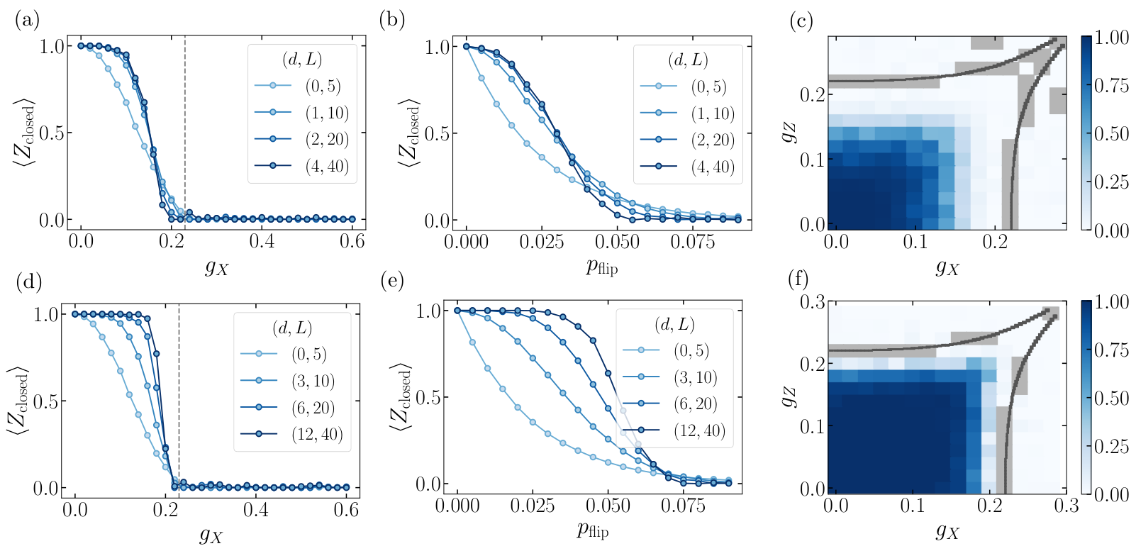
We now examine how different choices of LED decoders can change the size of the “correctable” region—that is, the region classified as topological. The main text demonstrates results for an (or ) patch-based decoder with coarse-graining size ; in Figure 15, we compare this with the pairing decoder and an () patch-based decoder which also uses . We see clearly that the and decoders both produce significantly larger correctable regions than the simple pairing decoder, for both coherent and incoherent errors. Meanwhile, the and decoders perform similarly, so it appears that the decoder threshold saturates with . Intriguingly, we observe saturation at an incoherent error rate which is significantly below the known error correction threshold of . An interesting open question is to determine whether this discrepancy arises because the patch-based decoder is suboptimal, or because local decoders have some fundamental limit. In the Supplementary Information, we show that a “annulus-based” decoder which applies MWPM in a non-local fashion results in a much larger correctable regime.
VIII.5 Definition and Properties of Fixed-Point States
As discussed in the main text, one important component for defining any LED procedure is to identify a fixed-point state of the target phase of matter. Here, we review the definition and key properties of a fixed-point state.
It is well-known in the literature that gapped quantum ground states can be classified by a real-space RG flow Chen et al. 2010; Schuch et al. 2011. To implement such an RG flow, one notes that any two states in the same phase can be connected by finite-depth local unitary transformations. The hallmark property of topologically-ordered states is the presence of long-range entanglement, and finite-depth local unitary transformations can add or remove local short-range entanglement; thus, for any given state in a topological phase of matter, one can construct a procedure which hierarchically removes all short-range entanglement from this state at increasing length-scales. Then, the resulting state then has zero correlation length, as all short-range entanglement has been removed; this state is known as a fixed-point state of the topological phase.
We also consider important properties of the fixed-point state in the context of our LED procedure and the closely related QCNN procedure of Ref. Cong et al. 2019. In both of these procedures, a fixed-point state of the phase under consideration is chosen, and the protocol identifies states within this phase by removing local errors or perturbations on top of this fixed-point state; this is done by performing a decoding operation and a coarse-graining operation, and repeating them times. In these settings, the fixed-point state has a few special properties: If the input state is equal to the fixed-point state, no errors are detected within each decoding step, and furthermore, the state after each layer of decoding and coarse-graining is equal to the input state, defined on a subsystem of the original system with fewer qubits. Finally, because fixed-point states have zero correlation length, the bare Wilson loops defined in the main text have expectation value equal to without performing any correction or LED.
VIII.6 LED Circuit for Toric Code
In the quantum circuit formulation, the stabilizer measurement, local decoding, and coarse-graining steps of LED are implemented through local controlled-unitary gates, single-qubit rotations, and (optionally) measurements and local feed-forward operations. Meanwhile, local variational unitary gates are introduced before each LED layer to enable efficient and robust identification of a large set of topologically-ordered states (see Methods and Figure 10). The quantum circuit for stabilizer measurements, local decoding, and coarse-graining can be implemented in different ways, as discussed below.
As a first example, one can introduce an ancillary qubit for each stabilizer, and perform local controlled-NOT (CNOT) gates between the system qubits and the ancillary qubit at each vertex or plaquette. These local CNOT gates are designed in the exact same fashion as stabilizer measurements of the surface code (see, for example, Ref. Fowler et al. 2012). Decoding can then be implemented either by measuring the ancillary qubits and performing local feed-forward operations on the system qubits to correct for arbitrary single-qubit errors, or by using local controlled-unitary operations between the ancillary and system qubits to achieve the same result. Finally, the MERA circuit of Ref. Aguado and Vidal 2008 can be used to perform coarse-graining at each LED layer.
Alternatively, one can avoid introducing ancillary qubits by carefully constructing a circuit which maps stabilizer values in each layer to the qubits which are removed during the coarse-graining process of that layer. This scheme combines the stabilizer measurement and coarse-graining procedures together into one large set of unitary operations. As before, the decoding step can be implemented by measuring stabilizer qubits and performing local feedforwarding to the remaining qubits, or by using local controlled-unitary operations between the ancillary and system qubits.
Because the number of removed qubits in each unit cell is always smaller than the number of stabilizers in this second case, only a fraction of stabilizers can be measured in every layer. Thus, one must design the circuit meticulously in order to still correct for all single-qubit errors. As a concrete example, we illustrate here such a quantum circuit implementation of the LED stabilizer measurement, local decoding, and coarse-graining procedures for the toric code which does not require additional ancillary qubits.
In this circuit, nine unit cells are combined to a single, large unit cell in the next layer by the coarse-graining procedure (i.e., a 3-to-1 reduction is performed in each dimension). The circuit is invariant under translation by the large unit cells, so we consider only the gates involving a single large unit cell. The setup and notations for qubits are defined in Figure 16.
Our circuit consists primarily of two-qubit CNOT gates, together with some single-qubit rotations and multi-qubit controlled-unitary operations. Thus, to compactly specify our circuit, we introduce some notations for the controlled-unitary operations of our circuit: specifically, we use the notation (control qubits target qubit) to refer to the gate which performs a bit-flip () gate on the target qubit if and only if all control qubits are in the state, and identity otherwise. For example, denotes a CNOT gate where is the control qubit and is the target qubit. Likewise, denotes a Toffoli gate where and are the control qubits and is the target qubit.
With all notations defined, we are now ready to specify our circuit. Due to translation invariance, it is understood that whenever we list a gate here, it will also be applied simultaneously on all qubits which differ from the labeled sites by translation of an integer number of large unit cells; thus, our circuit consists of many layers of non-overlapping local gates. The circuit proceeds as follows:
- 1.
Perform layers of CNOT gates in the following order: , , , , , , , , , , , , , , , , , , , , , , , , , , , , , .
- 2.
Perform layers of Toffoli gates in the following order: , , , .
- 3.
Perform single-qubit gates on , , , , , .
- 4.
Perform two layers of multi-qubit controlled-unitary gates ,
- 5.
Perform single-qubit Hadamard gates on , , , , , , , .
- 6.
Perform layers of Toffoli gates in the following order: , , , , , , , , , .
- 7.
Perform single-qubit Hadamard gates on and .
VIII.7 LED for Abelian Quantum Double Models

The snapshot-based LED framework can be extended to enable detection of Kitaev’s quantum double models based on any finite abelian group . Since the quantum double model of a direct product of finite groups is equivalent to the model where quantum doubles , …, are stacked together, it suffices to consider the quantum double of cyclic groups . In such models, an orientation must be assigned to each link of the square lattice, which is occupied by a qudit belonging to the Hilbert space spanned by (Figure 17). To define the vertex and plaquette stabilizers for these quantum double models, we first introduce the single-qudit shift and clock operators— and , respectively—which are generalizations of the Pauli matrices and for qubits. We define these operators based on their action on the basis states:
| (10) |
| (11) |
where addition is performed modulo , and is a root of unity. Using these operators, we can define generalized vertex and plaquette operators:
| (12) |
| (13) |
Here, the and operators depend on the orientation of the edge relative to the vertex or plaquette under consideration: if the directed edge points away from , , otherwise ; if is on the left (resp., right) of the directed edge when the lattice is rotated such that points upwards, (resp., ) Kitaev 2003. The Hamiltonian for this model is then
| (14) |
As in the case of the toric code Hamiltonian (Equation (1) in the main text), all and terms in the above Hamiltonian commute with each other. Each and has possible eigenvalues: 1, , , …, . The ground state(s) of are then simultaneous eigenstate(s) of all and . Meanwhile, vertex and plaquette violations correspond to anyonic excitations: a plaquette where hosts an anyon, while a vertex where hosts an anyon. Thus, at any site , there are possible topological charges ().
We now demonstrate how a generalized snapshot-based LED procedure can be used to recognize the quantum double phase. In this case, we begin by measuring all qudits in the basis , which we refer to as the group basis. Such a measurement allows us to compute all plaquette terms , and identify -type anyons. The location of such an anyon can be shifted one cell away by applying to one of the edges in (the sign depends on the edge’s orientation relative to the plaquette): for example, if the anyon is located on the plaquette in Figure 17, applying to will move the anyon up by one cell. The patch-based decoder we use for LED thus corrects errors by grouping together, when possible, two or more plaquettes with non-trivial such that the product ; this can be implemented simply by multiplying qudits by group elements . The groupings are chosen to minimize the total number of qudits to modify, while still removing as many errors as possible within each patch.
The above procedure allows us to correct for -type errors. The same LED procedure can be performed to address -type errors, by measuring qudits in another basis—the representation basis. Representation-basis measurements are performed by first applying a generalized Hadamard operator
| (15) |
and then measuring in the group basis. Because the shift operator is diagonal in the representation basis, measurements in this basis allow us to identify -type anyons, and utilize the patch-based decoding scheme described above for LED.
VIII.8 Background on Generic Topological Phases
Here, we provide background on generic topological quantum field theories (TQFTs), which are characterized by modular tensor categories . The possible topological charges (a.k.a. anyon types) in such a system are given by the simple objects of , where is the trivial or vacuum topological charge. Abelian anyons have quantum dimension , meaning that the outcome of fusing with any other anyon is deterministic: for some integer . On the other hand, non-abelian anyons have quantum dimensions , and their fusion can result multiple possible anyon types as governed by fusion rules
| (16) |
Here, the fusion coefficients must satisfy
| (17) |
Moreover, each anyon has a unique conjugate anyon for which (i.e., and can annihilate each other by fusing to vacuum); for all other , .
In addition to anyon types and fusion rules, several other quantities are needed to characterize a TQFT. In particular, for every pair of anyons , one can compute the Hopf link
| (18) |
Moreover, for each anyon , its topological twist is defined as
| (19) |
These quantities are used to define the modular and matrices of :
| (20) |
where is the global quantum dimension of .
It is conjectured that the modular and matrices uniquely define a unitary modular tensor category, or equivalently a topological phase of matter Wang 2010. In the main text and Methods, we illustrate the application of LED to Levin and Wen’s string-net models based on arbitrary unitary fusion categories . The MTC describing such a string-net model is the Drinfeld center Levin and Wen 2005. Additional background on general TQFTs and MTCs can be found in Refs. Bakalov and Kirillov 2001; Wang 2010.
VIII.9 Arbitrary Local Perturbations
In this section, we show that LED Wilson loops flow to one for any state which differs from the fixed-point state by an arbitrary local perturbation. This implies that LED loop operators are independent of the exact perturbation, unlike the fattened Wilson loops of Refs. Hastings and Wen 2005; Levin and Wen 2006. For concreteness, we examine perturbations on top of a toric code ground state.
To prove our claim, we consider a local unitary operator supported on a local region of diameter . It follows that can only flip a stabilizer from to if it overlaps with , and cannot couple any ground state to another ground state . We now show that LED removes all flipped stabilizers after layers, where is the coarse-graining length-scale. Because the coarse-graining step effectively reduces , after layers, there are three possibilities: (1) becomes fully contained within a single region at some layer . Then, has zero support after another layer of coarse-graining and disappears. (2) Before iteration , is supported on two adjacent regions. Then, becomes a single-qubit error after this iteration and is removed by the subsequent LED step. (3) Before iteration , is supported at the corner of three or four regions. In this case, it becomes a two-qubit diagonal error after this iteration, which can also be removed by the subsequent LED step. Notice that handling case (3) requires the inclusion of diagonal pairing in the pairing decoder. Finally, while this proof focuses on the pairing decoder, it also generalizes directly to more advanced local decoders, such as the patch-based decoder, when they are combined with coarse-graining.
VIII.10 Proof of Theorem 1
Theorem 1. Let be an arbitrary input state defined on a surface with trivial topology. Then, after performing LED with correction distance , assume the resultant state has, as a subsystem, qubits living on the links of a square lattice, as in the toric code. Then, if the stabilizer expectation values at every vertex and plaquette of the subsystem, then, the input state is topologically-ordered, in the sense that it is connected to an output state of the form by generalized local unitary (gLU) transformation of depth .
Proof.
The LED procedure forms a local quantum channel, and we begin our proof by constructing a purification of this channel. To mediate stabilizer measurement and local error correction, one can first introduce an ancilla in the state at every vertex and plaquette. Next, a sequence of Hadamard and controlled-NOT (CNOT) gates is applied such that a -basis measurement on an ancilla is equivalent to the associated stabilizer measurement of or . Then, local quantum error correction is performed using a local unitary evolution on the combined system, which contains the original state and the added ancilla qubits. This local unitary evolution applies gates which perform and spin flips on the system qubits, conditioned on the state of the ancilla qubits. Finally, the coarse-graining step can also be performed with local unitary transformations by using a quantum circuit corresponding to a multiscale entanglement renormalization ansatz (MERA) representation of the fixed-point state Aguado and Vidal 2008. The transformations generated by introducing product state ancillas and performing local unitary operations are called generalized local unitaries (gLU); this class of transformations includes our LED procedure described above and is known to preserve phase boundaries Chen et al. 2010.
If the system part of the final state, , has stabilizer expectation values at every vertex and plaquette , then must belong to the ground state space of the toric code. This is because the projector onto the ground state space is given by the product of all the stabilizers . On a surface with trivial topology, there is a unique state , so the output state factors into . ∎
VIII.11 Proof of Lemmas 3 and 4
Lemma 3. Given an output state satisfying the conditions of Theorem 2, and a simply connected square region on the system part, the reduced density matrix is indistinguishable from the toric code reduced density matrix defined on the same region, up to the bound
Proof.
To bound the trace distance, we will use the fact that our state locally looks almost the same as the toric code state. Specifically, trace distance is related to distinguishability by Nielsen and Chuang
| (21) |
To upper bound this, we can consider all possible unit norm operators . Specifically, can always be written as a linear combination of Pauli strings. These Pauli strings can be analyzed by considering two cases, closed strings and open strings. First consider operators supported on , which commute with all stabilizers supported on a slightly larger region (1-ball or ) , constructed by expanding on all sides by one unit cell. These operators must be products of contractible Wilson loops, and hence can be written as product of stabilizers. Therefore, for the toric code state. For the LED output state, we instead bound the expectation value of , where the product over (resp., ) runs over all vertices (plaquettes) within the region. The expectation value of this projector, evaluated on the output state, is given by . To lower bound this quantity, we first notice that every term in has spectrum , and that the terms are mutually commuting.
This allows us to approximate using the individual expectation values and . To do so, we note that if two commuting operators and , each with spectrum , satisfy and , then . To show this, we add the two individual bounds to obtain ; moreover, since has spectrum , we have . It thus follows that , and upon applying this recursively to include all vertex and plaquette terms within the region, we obtain .
Using this fact, along with we can similarly lower bound the expectation value . Thus, for any , we have .
Next, we consider operators which anti-commute with some stabilizers. In particular, these operators are Pauli strings with at least one endpoint (open strings). Naturally, their expectation value vanishes in the toric code state. To see this, let be one of the stabilizers which anti-commutes with . Now, and form an anti-commuting pair of Pauli operators, so they satisfy an uncertainty relation . As such, in the toric code where , this implies . Similarly, the condition leads to the upper bound . Combining these two results, we see the trace distance is at most . ∎
Lemma 4. Consider an input state and an LED procedure satisfying the conditions of Theorem 2. Then the final state after LED cannot be prepared using a local quantum circuit with depth less than .
To prove these results, we extend and generalize the proof techniques developed by Ref. Haah 2016. Note that for notional simplicity, here we work with an input state that is a purification of . This is done without loss of generality, since all of the operations act on the original degrees of freedom.
Consider a pair of -basis and -basis Wilson loops and , supported on two overlapping annuli. The twist product of the two operators is defined such that at one intersection region, operator is applied first, while at the other operator is applied first (Fig. 18). By the arguments of Ref. Haah 2016, such a pair of locally non-commuting observables, whose twist product does not factorize into a product of the individual observables, can serve as a witness for long-range entanglement. In our case, since - and -strings locally anti-commute, we can remove the twist to get .
Then, Ref. Haah 2016 showed that, assuming the observables and satisfy an additional important property called local invisibility (see below), then the following correlation serves as a witness for long-range order.
| (22) |
Specifically, the state cannot be prepared from a trivial state by a circuit of depth , where is the separation between the two intersection regions. Indeed, in the exact case, where the expectation value of large LED Wilson loops are one, the results of Ref. Haah 2016 can be directly applied.
However, the proofs in Ref. Haah 2016 do not immediately apply to the realistic case considered here, where stabilizers have expectation value , and residual entanglement between the system and ancilla or environment qubits prevents exact knowledge of the state. Nevertheless, with sufficient care and a few additional assumptions, approximate versions of key results in Ref. Haah 2016 can be recovered.
First, we develop a notion of approximate local invisibility. Throughout, we follow the spirit of the proofs in Section III of Ref. Haah 2016; the reader is encouraged to consult the original reference for additional details and insights.
Definition 5 (Approximate ()-local invisibility.).
Let be a region of radius and be a -ball around . An operator with unit norm is ()-locally invisible with respect to a state if, for any state whose reduced density matrix on is equivalent to , it satisfies
| (23) |
where the norm is the standard trace norm. In other words, locally invisible operators leave local reduced density matrices approximately unchanged. Note that we restrict to states for which the expectation value does not vanish, such that this remains well-defined. This subtlety is also present in the original definition of Ref. Haah 2016.
Next, we will show that Wilson loops that nearly stabilize are approximately locally invisible. Let be a region of radius , which can only cover a patch of the loop. Furthermore, let , i.e. region is identical to region . Since the Wilson loop is a tensor product of local unitaries, we can write and . This allows us to work directly with the reduced density matrices of region , and we can use Lemma 3 to reduce to the toric code case
| (24) |
Indeed, since is locally invisible with respect to to the toric code, this gives us our result, where the error term depends on the size of .
| (25) |
More microscopically, spans the region, so locally looks like a logical operator. The reduced density matrix on region is an equal weight mixture of all logical states, so leaves it invariant.
This shows that Wilson loops are ()-locally invisible with respect to for and . When combined with the fact that Wilson loops have large expectation value on , this will serve as a witness for long-range topological order.
To prove this, we need to confirm that, even for the weaker notion of approximate local invisibility, the twist product approximately factorizes for trivial states.
Lemma 6.
The twist product of two locally invisible operators and , acting on a trivial product state , must satisfy
| (26) |
where and are supported on two annuli which intersect at two regions (Fig. 18) whose separation is .
Proof.
In the first step of the proof, we bound the expectation value of , the projector onto supported on region evaluated with respect to for unitary .
Invoking the definition of local invisibility, we show for of radius , that .
| (27) |
Thus, the expectation value of the observable satisfies:
| (28) | ||||
| (29) |
Next, we can use the fact that can be written as a product of approximately times. It follows from the same union bound argument in Lemma 3, that . This result can be used to bound the distance between the two states,
| (30) |
by noticing the left side is equal to . We will use this below, to show that we can replace with without incurring significant error.
To prove the main result, we use the same construction as Ref. Haah 2016. Specifically, we want to use the above result to show that . We do this by carefully inserting projectors. For Wilson loops, which are tensor product operators, we the twist product can be split up as follows (see Fig. 18),
| (31) |
Our above result implies . We can subsequently pull projectors from to cover the region of support of , e.g. low and the parts of high. Thus, we get
| (32) | ||||
as we wanted. Finally, we this implies the expectation value of the twist product approximately factorizes . ∎
Although we proved that the twist product must factorize for the trivial product state, this holds for a much wider class of short-range entangled states, generated from a trivial state by a finite-depth unitary circuit. In particular, using the same argument as Haah Lemma III.3 shows that, given a ()-locally invisible operator and state , if we evolve under a local unitary circuit of depth , then the operator is -locally indistinguishable with respect to . This will be used to show that non-factorizability of the twist product lower bounds the depth of a quantum circuit required to produce the state from the trivial product state.
Finally, we can use the trace distance Lemma 3, to show the twist product does not factorize for . Specifically, let and be Wilson loops supported on an region. Then,
| (33) |
for a constant . Combining this Lemma 6 for trivial states, we see the bound is violated when
| (34) | ||||
| (35) |
We choose to be a constant fraction of , and see that we can roughly make and still certify long-range order. In particular, the state cannot be generated by a finite depth circuit of depth smaller than . Since is connected to the input state by a depth- quantum circuit, this implies LED Wilson loops close to one certify topological order up to length-scales .
VIII.12 Connection Between LED and Entanglement Negativity
The LED framework suggests a characterization of topological order based on the ability to distill the fixed-point wavefunction using generalized local unitary operations. In this section, we connect this definition to the topological entanglement negativity of the input state, a typical observable used to detect topological order in mixed states Peres 1996; Horodecki et al. 1996.
As described above, the circuit construction for LED involves applying local unitary transformations to the input mixed state and product state ancillas . States that are classified as topological by LED are connected via a finite-depth local unitary to the toric code fixed-point state and an ancillary register (see Theorem 1).
In particular, all of the entropy in the input state, associated with both incoherent and coherent fluctuations away from the fixed point state, is transferred to the ancilla .
We conjecture that the ability to “distill” the toric-code fixed point state also implies the presence of a topological correction to the entanglement negativity of the input state. Although we cannot prove this statement rigorously, we make the connection more precise in this section. First, we make the plausible assumption that the ancilla is in a trivial mixed state. This ensures all of the topological contribution to the entanglement negativity comes from the system part . Then, we argue the topological contribution remains after applying inverse LED circuits (coarsening of the Wilson loops). In particular, if we consider local Clifford circuits, we can show this is indeed the case. Together, these arguments suggest that the topological order witness provided by LED should also serve as a witness for other quantities like entanglement negativity in many scenarios of practical interest.
The key assumption we make is that the ancilla is in a trivial mixed state. Concretely, we assume that there exists a local purification of which is connected to a product state under local unitary circuits (Figure 19). This local purification is constructed by doubling the number of qubits, such that . Here, is the subsystem which implements the purification. Qubits in are placed next to qubits in , so that the local structure is preserved. Then, we assume that there is a local unitary which maps to a product state. Thus, can be “locally purified” to a product state. We note that in the circuit model, the assumption about may be checkable via state tomography.
Taking into account the purified register of qubits, the output state can now be written as a pure state. Further, it is a stabilizer state, with toric code stabilizers for the subsystem, and trivial stabilizers for the combined subsystem. Note we assume for simplicity a topologically trivial manifold, so there are no non-trivial logical operators. Our construction then implies that this stabilizer state is connected to a purification of the input state via local unitary circuits. If we then trace out the degrees of freedom associated with , this produces the input mixed state. We can leverage the stabilizer structure to make concrete statements about the entanglement negativity of this input mixed state.
First, we review the calculation of the entanglement negativity from Ref. Lu and Vijay 2022, for the toric code output state. Consider a partition of the system into region and its complement . Note that is associated with a region of space, and hence contains sites from all three subsystems , , and . The entanglement negativity is given by , where is the partial transpose of the output density matrix, and are the associated eigenvalues. The partial transpose of the density matrix , which is defined as
| (36) | |||
| (37) |
where and form an orthonormal basis for the two parts of the system. To start, notice that the only non-zero eigenvalue of the bare output state corresponds to the simultaneous eigenstate of all the stabilizers, , and .
Under the inverse LED operations, each individual stabilizer is coarsened, making exact computation of the entanglement negativity difficult. However, the LED circuit provides additional structure. Importantly, the toric code stabilizers map onto the system part. These become the LED Wilson loops which we measure in the input state. In contrast, the trivial stabilizers can also map onto subsystem that will be traced out. As a result, we expect the coarsened toric code stabilizers will still contribute a topological term in the entanglement negativity. We conjecture this is true for any local unitary circuit. However, we are able to calculate it if we consider the specific case of local Clifford circuits. Note that the LED circuits which implement local pairing decoders are not Clifford circuits, and hence the argument does not rigorously apply in that case.
Let label the toric code stabilizers in the original state, and the stabilizers of the ancilla. Under the Clifford unitary, these stabilizers are mapped to coarsened versions, .
The reduced density matrix of the input state, before tracing out the auxilliary qubits, can be written as
| (38) |
Suppose there are stabilizers and an equivalent number of qubits. This is the case if we are working on a topologically trivially manifold. Then, has a unique non-vanishing eigenstate with eigenvalue one. Thus, . Following Ref. Lu and Vijay 2022, we can equivalently write
| (39) |
Next, consider splitting the system into two regions, and , and take the partial transpose of on .
| (40) |
The key to computing the entanglement negativity is to simplify .
In the output state, which is simply the toric code state with product state ancillas, the entanglement negativity can be exactly computed, and has been shown to have a topological correction coming from the long-range topological order Lee and Vidal 2013; Lu and Vijay 2022. We extend this computation to show the topological correction survives upon performing local Clifford circuits and tracing out the ancillary degrees of freedom.
We start by reviewing the computation in the output, fixed-point state. The first thing to notice is that trivially commutes with and , because they are supported on different qubits. Second, is invariant under partial transpose, since the operators are supported on a single site and hence cannot span the boundary between and . Thus, we can pull the out from the product.
Next, we discuss the effect of partial transpose on the toric code stabilizers, following Ref. Lu and Vijay 2022. The only stabilizers which are affected non-trivially are those that span the boundary. In particular, if we consider a pair of stabilizers and that intersect at two sites, but only one of the sites is supported in , then they pick up a minus sign under partial transpose (see Figure 20). More generally, picks up an overall sign if the number of such intersections is odd.
We can now discuss the spectrum of the partially transposed density matrix. Note that an orthonormal basis for the Hilbert space can be formed from simultaneous eigenstates of all the stabilizers. These states are labelled by the stabilizer eigenvalues, which can be . For non-trivial eigenstates of , stabilizers which are unaffected by partial transpose must have eigenvalue one. Thus, we can reduce the spectrum calculation to only stabilizers on the boundary.
Therefore, we can associate eigenstates with expectation values of “strange correlators” of the form Lu and Vijay 2022. Order stabilizers around the boundary, so are on even sites and on odd sites, and consider specifically the correlators,
Here, is a wavefunction that encodes the signs coming from partial transpose, and is a uniform superposition over all configurations. The wavefunction for is the same as the 1D cluster state. Non-vanishing correlators are generated by products of and , the stabilizers of the cluster state. There are of such non-vanishing correlators, each with expectation value . The overlap is , where . Thus, the entanglement negativity is where is the size of the perimeter. The constant correction is a signature of topological entanglement entropy.
Next, we discuss how the effect of finite-depth Clifford circuits on the entanglement negativity. In particular, since Clifford circuits map stabilizers to stabilizers, eigenstates of can still be labelled by stabilizer expectation values, and the entanglement negativity can be calculated by enumerating non-zero strange correlators. However, a few important things change. The set of stabilizers which span the boundary, and hence may have non-trivial twist products with other stabilizers, is considerably larger. Any or stabilizer that is within distance of the boundary could contribute. Applying the same procedure as in the case of the toric code, we can enumerate non-trivial strange correlators of the form for a different state . However, now the Hilbert space of has one qubit associated with each relevant , or .
Now, we argue that new state preserves the same cluster-state structure as in the fixed-point case and still has long-range SPT order. First, we show that still has a symmetry, generated by the product of Pauli- operators on all qubits associated with , or all qubits associated with . To see this, notice that the product of all relevant decomposes into two independent Wilson loops, each supported distance away from the boundary on the interior and exterior sides. Each of these Wilson loops individually has trivial twist-product with the other transformed stabilizers, implying that it can be applied (on either side) to the partially-transposed state without changing the state. This further implies that is invariant under applying the Pauli- associated with each qubit.
Second, we show that there exists long-range SPT order in . In particular, to do this, we show that there are coarse-grained stabilizers which have the same behavior under partial transpose as the stabilizers at the toric-code fixed point. Consider large Wilson loops generated by multiplying either or in a large contiguous region spanning the boundary (see Figure 20). In particular, if we look at regions that are offset, the large Wilson loops associated with or necessarily anti-commute on either side of the boundary, leading to a twist product of . Therefore, we can construct coarse-grained Pauli-‘’ and ‘’ operators in the Hilbert space of simply by taking products of single-qubit Pauli operators. This argument shows that the coarse-grained operator is a stabilizer of the state.
Finally, we discuss the effect of the remaining degrees of freedom on the entanglement negativity. The stabilizers split into two groups: those that contain support on , and those that are fully supported on . Let us start with the first group. Since we trace out all of subsystem , the effect on the stabilizers is to replace the stabilizer state with the maximally mixed state
| (41) |
The operator has two eigenvectors, each with eigenvalue 1/2. Thus, any stabilizer with support on becomes fully disentangled from the rest of the system, and has no effect on the entanglement negativity. Next, consider stabilizers that are fully supported on . The which are near the boundary between and will potentially contribute to the entanglement negativity. Furthermore, they may have non-trivial commutation with , , and other after partial transposition. Thus, they can contribute to the topological entanglement entropy. However, since only operators near the boundary are affected by partial transpose, these operators only contribute an area-law contribution. Further, we note that they cannot change the long-range SPT order of , since they commute with the symmetry. As such, they also should not affect the value of the topological term.
The argument presented above relied on the fact that the stabilizers of the state were Pauli operators. This meant the spectrum of could be exactly computed, and the techniques of Ref. Lu and Vijay 2022 could be applied. However, the key part of the proof involved generating a sub-algebra of coarse-grained Wilson loops with twist-product . LED provides a constructive method for measuring such coarse-grained Wilson loops, with non-trivial twist products, in generic mixed states, as explained in our proof of Theorem 1. Hence, it would be interesting to directly link the existence of operators with non-trivial twist product to the topological entanglement negativity in general mixed states.
VIII.13 Valence-Bond Solid Phase
In the main text, we argued that the flow of closed-loop and open-string Wilson operators suggest that the large regime is most consistent with a decoherence-dominated disorder phase. This in contrast to numerical simulations, which suggest the ground state in this regime is a valance bond solid (VBS) state Verresen et al. 2021a. The VBS fixed-point state can be understood as a single dimer covering, in contrast to the spin-liquid state which is a uniform superposition over dimer coverings. More generally, in VBS phase the -anyons become condensed and the -anyons become confined. As such, in the VBS phase, we would expect that closed -loops flow to , and open -strings flow to either or depending on how many dimers they intersect. However, our analysis shows that all -loops, both open and closed, stay near zero under LED flow. In the main text, we average over all open -strings, so the vanishing signal could be due to cancellation of individual loops that flow to opposite values. In Figure 21, we also plot a representative, single -string, and see the expectation value still remains close to zero at large . Since the -loops also remain at zero, this is the same signature of the high incoherent error regime of the toric code mixed-state phase diagram.
VIII.14 Detecting Gauge-Glass Phases and More
The LED techniques developed here can also be applied to characterize generalized toric code orders in higher dimensions. The 2D toric code we study has point-like excitations. However, different models can have higher-dimensional excitations, such as line-like excitations appearing in the 2D Ising model and 3D gauge theories. LED can also be applied in these cases. In particular, simple local decoders for models with line-like excitations also exist. For example Toom’s rule, as described in Ref. Breuckmann et al. 2016, can be made into a local decoder by restricting the number of update steps to some constant. The patch-based decoder can also be generalized to this case by locally identifying small contractible loops. Another strategy would be to consider spatial slices of the model with line-like excitations. This would result in a lower-dimensional model with point-like excitations, for which the techniques presented in this paper can be directly applied.
A particularly interesting case study is the 3D random-plaquette gauge model. The degrees of freedom live on the links of the 3D square lattice. Products of spin operators around each plaquette measure the magnetic flux. Excitations are line-like magnetic flux tubes, coming from chains of excited plaquettes. The model also has quenched disorder, so that the zero-temperature state has a finite density of magnetic flux tubes. Hence, there are two sources of flux tubes, the quenched disorder as well as thermal fluctuations. Due to the gauge constraints, the combination of flux tubes from quenched disorder and thermal fluctuations always form closed loops.
Let be the parameter which determines the density of quenched disorder, and the effective temperature. The model has three phases of interest to us. The first is an ordered phase for small and , where the density of flux tubes is small. The second is a disordered phase at large and , where flux tubes condense. These two phases can be distinguished by measuring the disorder averaged Wilson loop . In Ref. Wang et al. 2003, it is suggested that these two phases be identified by comparing perimeter-law decay vs. area-law decay in each of the distinct phases. Perimeter-law decay indicates that the fluctuations which cause the Wilson loop to decay are local, and hence characterizes the ordered phase.
The third phase is a disordered but glassy phase at large but small . In this phase, quenched disorder is large, leading to a high density of flux tubes. As a result, the disorder averaged Wilson loop obeys an area-law, consistent with a disordered phase. However, thermal fluctuations remain small, and the pattern of flux tubes is static when averaged over thermal fluctuations. Therefore, the square of the thermal expectation value, , should decay as perimeter-law and can hence distinguish the disordered phase from the glassy phase.
The LED observables we construct here can be used to more robustly classify these phases as well. In particular, as explained in the main text, differentiating between perimeter-law and area-law is difficult in practice. Both of these signals decay exponentially in loop size, causing the sample complexity to increase significantly. Further, area-law generically becomes mixed with perimeter-law in the presence of additional imperfections or perturbations, such as incoherent errors or gauge-constraint violating terms. However, using LED, the Wilson loops will be amplified to one only in the ordered phase. Similarly, the squared Wilson loop would be amplified in the ordered and glassy phases. This observable can also be efficiently measured from snapshots, as long as we are able to sample multiple times from each quenched disorder realization. Another strategy, which could be more sample efficient, is the following: Given two independent snapshots from the same quenched disorder realization, one can compute the element-wise sum modulo two, , and then measure the LED Wilson loop on the new snapshot . Intuitively, such a procedure effectively removes the quenched disorder, which is fixed from snapshot-to-snapshot, leaving behind only the thermal fluctuations. Identifying such gauge-glassy models is also difficult in numerical simulations, and hence LED and related ideas could also be applicable in those contexts.
VIII.15 Annulus Decoders
In this section, we consider an alternative approach to constructing error corrected operators, by applying MWPM to an annulus. Anyons supported on the annulus can be paired either with other anyons, or with the boundary of the annulus. Interestingly, MWPM is a global decoder, where introducing or removing anyons can change the pairing far away. However, by construction, the decoder cannot connect the interior of the annulus to the exterior.
We show in Figure 22 the behavior of these corrected loop operators for coherent, incoherent, and mixed errors. In particular, for the incoherent error model, we see the region classified as topological seems to coincide with the known error recovery threshold of for MWPM. This is much closer to the theoretical optimal error correction threshold of , where we expect the phase transition from topological to disordered to occur.
Since this decoder is non-local, our existing theoretical arguments, and the connection to RG, may not apply. Nevertheless, an annulus decoder cannot change the super-selection sector—whether or not an anyon is contained within the annulus. Therefore, if the annulus-correction decorated loops go to one, then asymptotically large regions have well-defined super-selection sectors, suggesting the state is topologically-ordered. Indeed, it has been argued that such an annulus decoder could be considered a witness for topological entanglement entropy Wootton 2012.
Competing Interests. M.D.L. is a co-founder and shareholder of QuEra Computing.
Data Availability Statement. The data that support the plots within this paper and other findings of this study are available from the corresponding author upon reasonable request.
Code Availability Statement. The code used to generate the plots within this paper and other findings of this study are available from the corresponding author upon reasonable request.
Acknowledgments. We thank E. Altman, Y. Bao, D. Bluvstein, Z.-P. Cian, S. Ebadi, G. Giudici, M. Hafezi, H.-Y. Huang, A. Kitaev, H. Levine, J. Preskill, S. Sachdev, R. Sahay, N. Tantivasadakarn, R. Verresen, A. Vishwanath, T. T. Wang, and X.-G. Wen for insightful discussions, and we especially thank D. Aasen and Z. Wang for providing helpful information and conversations on applying LED to non-abelian topological phases. We also thank the Referee for the suggestion to consider gauge-glassy models. This work was supported by the US Department of Energy [DE-SC0021013 and DOE Quantum Systems Accelerator Center (contract no. 7568717)], the Defense Advanced Research Projects Agency (grant no. W911NF2010021), the National Science Foundation, the Department of Defense Multidisciplinary University Research Initiative (ARO MURI, grant no. W911NF2010082), and the Harvard-MIT Center for Ultracold Atoms. I.C. acknowledges support from the Alfred Spector and Rhonda Kost Fellowship of the Hertz Foundation, the Paul and Daisy Soros Fellowship, and the Department of Defense through the National Defense Science and Engineering Graduate Fellowship Program. N.M. acknowledges support from the Department of Energy Computational Science Graduate Fellowship under Award Number DE-SC0021110. HP acknowledges support from the ERC Starting grant no. 101041435 and the Erwin Schrödinger Center for Quantum Science and Technology.
References
- Wen (2017) X.-G. Wen, “Colloquium: Zoo of quantum-topological phases of matter,” Rev. Mod. Phys. 89, 041004 (2017), publisher: American Physical Society.
- Nayak et al. (2008) C. Nayak, S. H. Simon, A. Stern, M. Freedman, and S. Das Sarma, “Non-abelian anyons and topological quantum computation,” Rev. Mod. Phys. 80, 1083–1159 (2008).
- Terhal (2015) B. M. Terhal, “Quantum error correction for quantum memories,” Rev. Mod. Phys. 87, 307–346 (2015).
- Sachdev (1992) S. Sachdev, “Kagome- and triangular-lattice Heisenberg antiferromagnets: Ordering from quantum fluctuations and quantum-disordered ground states with unconfined bosonic spinons,” Phys. Rev. B 45, 12377–12396 (1992), publisher: American Physical Society.
- Hastings and Wen (2005) M. B. Hastings and X.-G. Wen, “Quasiadiabatic continuation of quantum states: The stability of topological ground-state degeneracy and emergent gauge invariance,” Phys. Rev. B 72, 045141 (2005), publisher: American Physical Society.
- Wilson (1974) K. G. Wilson, “Confinement of quarks,” Physical Review D 10, 2445–2459 (1974).
- Haah (2016) J. Haah, “An invariant of topologically ordered states under local unitary transformations,” Communications in Mathematical Physics 342, 771–801 (2016), publisher: Springer.
- Kitaev (2003) A. Kitaev, “Fault-tolerant quantum computation by anyons,” Annals of Physics 303, 2–30 (2003), publisher: Elsevier BV.
- Bridgeman et al. (2016) J. C. Bridgeman, S. T. Flammia, and D. Poulin, “Detecting topological order with ribbon operators,” Physical Review B 94, 205123 (2016).
- Iqbal and Schuch (2021) M. Iqbal and N. Schuch, “Entanglement Order Parameters and Critical Behavior for Topological Phase Transitions and Beyond,” Physical Review X 11, 041014 (2021).
- Duivenvoorden et al. (2017) K. Duivenvoorden, M. Iqbal, J. Haegeman, F. Verstraete, and N. Schuch, “Entanglement phases as holographic duals of anyon condensates,” Phys. Rev. B 95, 235119 (2017).
- Jamadagni et al. (2022) A. Jamadagni, J. Kazemi, and H. Weimer, “Learning of error statistics for the detection of quantum phases,” (2022).
- Kitaev and Preskill (2006) A. Kitaev and J. Preskill, “Topological Entanglement Entropy,” Phys. Rev. Lett. 96, 110404 (2006), publisher: American Physical Society.
- Levin and Wen (2006) M. Levin and X.-G. Wen, “Detecting Topological Order in a Ground State Wave Function,” Phys. Rev. Lett. 96, 110405 (2006), publisher: American Physical Society.
- Schuch et al. (2011) N. Schuch, D. Pérez-García, and I. Cirac, “Classifying quantum phases using matrix product states and projected entangled pair states,” Phys. Rev. B 84, 165139 (2011).
- Chen et al. (2011) X. Chen, Z.-C. Gu, and X.-G. Wen, “Classification of gapped symmetric phases in one-dimensional spin systems,” Phys. Rev. B 83, 035107 (2011).
- Cong et al. (2019) I. Cong, S. Choi, and M. D. Lukin, “Quantum convolutional neural networks,” Nature Physics 15, 1273–1278 (2019), publisher: Nature Publishing Group.
- Chen et al. (2010) X. Chen, Z.-C. Gu, and X.-G. Wen, “Local unitary transformation, long-range quantum entanglement, wave function renormalization, and topological order,” Physical Review B 82, 155138 (2010).
- Haegeman et al. (2015) J. Haegeman, K. Van Acoleyen, N. Schuch, J. I. Cirac, and F. Verstraete, “Gauging quantum states: From global to local symmetries in many-body systems,” Phys. Rev. X 5, 011024 (2015).
- Zhu and Zhang (2019) G.-Y. Zhu and G.-M. Zhang, “Gapless coulomb state emerging from a self-dual topological tensor-network state,” Phys. Rev. Lett. 122, 176401 (2019).
- Castelnovo and Chamon (2008) C. Castelnovo and C. Chamon, “Quantum topological phase transition at the microscopic level,” Physical Review B 77, 054433 (2008).
- Haah et al. (2017) J. Haah, A. W. Harrow, Z. Ji, X. Wu, and N. Yu, “Sample-optimal tomography of quantum states,” IEEE Transactions on Information Theory 63, 5628–5641 (2017).
- Dennis et al. (2002) E. Dennis, A. Kitaev, A. Landahl, and J. Preskill, “Topological quantum memory,” Journal of Mathematical Physics 43, 4452–4505 (2002), publisher: American Institute of Physics.
- Fredenhagen and Marcu (1983) K. Fredenhagen and M. Marcu, “Charged states in gauge theories,” Communications in Mathematical Physics 92, 81–119 (1983).
- Peres (1996) A. Peres, “Separability Criterion for Density Matrices,” Physical Review Letters 77, 1413–1415 (1996).
- Horodecki et al. (1996) M. Horodecki, P. Horodecki, and R. Horodecki, “Separability of mixed states: necessary and sufficient conditions,” Physics Letters A 223, 1–8 (1996).
- Lee and Vidal (2013) Y. A. Lee and G. Vidal, “Entanglement negativity and topological order,” Physical Review A 88, 042318 (2013).
- Semeghini et al. (2021) G. Semeghini, H. Levine, A. Keesling, S. Ebadi, T. T. Wang, D. Bluvstein, R. Verresen, H. Pichler, M. Kalinowski, R. Samajdar, et al., “Probing topological spin liquids on a programmable quantum simulator,” Science 374, 1242–1247 (2021).
- Verresen et al. (2021a) R. Verresen, M. D. Lukin, and A. Vishwanath, “Prediction of toric code topological order from Rydberg blockade,” Phys. Rev. X 11, 031005 (2021a).
- Saffman et al. (2010) M. Saffman, T. G. Walker, and K. Mølmer, “Quantum information with rydberg atoms,” Rev. Mod. Phys. 82, 2313–2363 (2010).
- Misguich et al. (2002) G. Misguich, D. Serban, and V. Pasquier, “Quantum Dimer Model on the Kagome Lattice: Solvable Dimer-Liquid and Ising Gauge Theory,” Phys. Rev. Lett. 89, 137202 (2002), publisher: American Physical Society.
- Poilblanc et al. (2012) D. Poilblanc, N. Schuch, D. Pérez-García, and J. I. Cirac, “Topological and entanglement properties of resonating valence bond wave functions,” Phys. Rev. B 86, 014404 (2012), publisher: American Physical Society.
- Samajdar et al. (2022) R. Samajdar, D. G. Joshi, Y. Teng, and S. Sachdev, “Emergent gauge theories and topological excitations in Rydberg atom arrays,” (2022).
- Tarabunga et al. (2022) P. S. Tarabunga, F. M. Surace, R. Andreoni, A. Angelone, and M. Dalmonte, “Gauge-theoretic origin of rydberg quantum spin liquids,” (2022).
- Verresen and Vishwanath (2022) R. Verresen and A. Vishwanath, “Unifying Kitaev magnets, kagome dimer models and ruby Rydberg spin liquids,” (2022).
- Bricmont and Frölich (1983) J. Bricmont and J. Frölich, “An order parameter distinguishing between different phases of lattice gauge theories with matter fields,” Physics Letters B 122, 73–77 (1983).
- Gregor et al. (2011) K. Gregor, D. A. Huse, R. Moessner, and S. L. Sondhi, “Diagnosing deconfinement and topological order,” New Journal of Physics 13, 025009 (2011).
- Zhu et al. (2020) G. Zhu, A. Lavasani, and M. Barkeshli, “Universal logical gates on topologically encoded qubits via constant-depth unitary circuits,” Phys. Rev. Lett. 125, 050502 (2020).
- König et al. (2009) R. König, B. W. Reichardt, and G. Vidal, “Exact entanglement renormalization for string-net models,” Phys. Rev. B 79, 195123 (2009).
- Levin and Wen (2005) M. A. Levin and X.-G. Wen, “String-net condensation: A physical mechanism for topological phases,” Phys. Rev. B 71, 045110 (2005).
- Wang (2010) Z. Wang, Topological quantum computation, 112 (American Mathematical Soc., 2010).
- Bakalov and Kirillov (2001) B. Bakalov and A. A. Kirillov, Lectures on tensor categories and modular functors, Vol. 21 (American Mathematical Soc., 2001).
- Huang et al. (2022) H.-Y. Huang, R. Kueng, G. Torlai, V. V. Albert, and J. Preskill, “Provably efficient machine learning for quantum many-body problems,” Science 377, eabk3333 (2022).
- Wang et al. (2003) C. Wang, J. Harrington, and J. Preskill, “Confinement-higgs transition in a disordered gauge theory and the accuracy threshold for quantum memory,” Annals of Physics 303, 31–58 (2003).
- Satzinger et al. (2021) K. Satzinger, Y.-J. Liu, A. Smith, C. Knapp, M. Newman, C. Jones, Z. Chen, C. Quintana, X. Mi, A. Dunsworth, et al., “Realizing topologically ordered states on a quantum processor,” Science 374, 1237–1241 (2021).
- Stricker et al. (2020) R. Stricker, D. Vodola, A. Erhard, L. Postler, M. Meth, M. Ringbauer, P. Schindler, T. Monz, M. Müller, and R. Blatt, “Experimental deterministic correction of qubit loss,” Nature 585, 207–210 (2020).
- Jamadagni and Weimer (2022) A. Jamadagni and H. Weimer, “Operational definition of topological order,” Phys. Rev. B 106, 085143 (2022).
- Bao et al. (2023) Y. Bao, R. Fan, A. Vishwanath, and E. Altman, “Mixed-state topological order and the errorfield double formulation of decoherence-induced transitions,” (2023), arXiv:2301.05687 [quant-ph] .
- Hastings (2011) M. B. Hastings, “Topological order at nonzero temperature,” Phys. Rev. Lett. 107, 210501 (2011).
- Verresen et al. (2021b) R. Verresen, N. Tantivasadakarn, and A. Vishwanath, “Efficiently preparing Schrödinger’s cat, fractons and non-abelian topological order in quantum devices,” (2021b).
- Schuch et al. (2012) N. Schuch, D. Poilblanc, J. I. Cirac, and D. Pérez-García, “Resonating valence bond states in the PEPS formalism,” Phys. Rev. B 86, 115108 (2012), publisher: American Physical Society.
- Schuch et al. (2007) N. Schuch, M. M. Wolf, F. Verstraete, and J. I. Cirac, “Computational complexity of projected entangled pair states,” Phys. Rev. Lett. 98, 140506 (2007).
- Cirac et al. (2021) J. I. Cirac, D. Pérez-García, N. Schuch, and F. Verstraete, “Matrix product states and projected entangled pair states: Concepts, symmetries, theorems,” Rev. Mod. Phys. 93, 045003 (2021).
- Napp et al. (2022) J. C. Napp, R. L. La Placa, A. M. Dalzell, F. G. S. L. Brandão, and A. W. Harrow, “Efficient classical simulation of random shallow 2d quantum circuits,” Phys. Rev. X 12, 021021 (2022).
- Vidal (2008) G. Vidal, “Class of quantum many-body states that can be efficiently simulated,” Phys. Rev. Lett. 101, 110501 (2008).
- Duclos-Cianci and Poulin (2013) G. Duclos-Cianci and D. Poulin, “Fault-tolerant renormalization group decoder for abelian topological codes,” (2013), 10.48550/ARXIV.1304.6100.
- Fowler et al. (2012) A. G. Fowler, M. Mariantoni, J. M. Martinis, and A. N. Cleland, “Surface codes: Towards practical large-scale quantum computation,” Phys. Rev. A 86, 032324 (2012).
- McClean et al. (2018) J. R. McClean, S. Boixo, V. N. Smelyanskiy, R. Babbush, and H. Neven, “Barren plateaus in quantum neural network training landscapes,” Nature communications 9, 1–6 (2018).
- Pesah et al. (2021) A. Pesah, M. Cerezo, S. Wang, T. Volkoff, A. T. Sornborger, and P. J. Coles, “Absence of barren plateaus in quantum convolutional neural networks,” Phys. Rev. X 11, 041011 (2021).
- Lu and Vijay (2022) T.-C. Lu and S. Vijay, “Characterizing long-range entanglement in a mixed state through an emergent order on the entangling surface,” (2022), 10.48550/ARXIV.2201.07792.
- Fan et al. (2023) R. Fan, Y. Bao, E. Altman, and A. Vishwanath, “Diagnostics of mixed-state topological order and breakdown of quantum memory,” (2023), arXiv:2301.05689 [quant-ph] .
- Aguado and Vidal (2008) M. Aguado and G. Vidal, “Entanglement renormalization and topological order,” Phys. Rev. Lett. 100, 070404 (2008).
- (63) M. A. Nielsen and I. L. Chuang, Quantum Computation and Quantum Information: 10th Anniversary Edition.
- Breuckmann et al. (2016) N. P. Breuckmann, K. Duivenvoorden, D. Michels, and B. M. Terhal, “Local decoders for the 2d and 4d toric code,” (2016), 10.48550/ARXIV.1609.00510.
- Wootton (2012) J. R. Wootton, “A witness for topological order and stable quantum memories in abelian anyonic systems,” Journal of Physics A: Mathematical and Theoretical 45, 395301 (2012).
- Giudici et al. (2022) G. Giudici, M. D. Lukin, and H. Pichler, “Dynamical preparation of quantum spin liquids in Rydberg atom arrays,” (2022).
- Cheng et al. (2021) Y. Cheng, C. Li, and H. Zhai, “Variational approach to quantum spin liquid in a Rydberg atom simulator,” (2021).
apsrev41Control