Visual perception and language understanding are - fundamental components of human intelligence, enabling them to understand and reason about objects and their interactions. It is crucial for machines to have this capacity to reason using these two modalities to invent new robot-human collaborative systems.

Recent advances in deep learning have built separate sophisticated representations of both visual scenes and languages. However, understanding the associations between the two modalities in a shared context for multimodal reasoning remains a challenge. Focusing on language and vision modalities, this thesis advances understanding of how to exploit and use pivotal aspects of vision-and-language tasks with neural networks to support reasoning. The contributions include: (i) effective mechanisms for content selection and construction of temporal relations from dynamic visual scenes in response to a linguistic query and preparing adequate knowledge for the reasoning process (ii) new frameworks to perform reasoning with neural networks by exploiting visual-linguistic associations, deduced either directly from data or guided by external priors.

In the first work, we present a novel dual process neural architecture resembling the dual process in the human reasoning systems for Video Question Answering (Video QA). It is composed of a question-guided video process module that is fast and reactive (System 1) followed by a generic reasoning module that is slow and deliberative (System 2). The fast system is a hierarchical model that encodes visual patterns about objects, actions and relations in space-time given the textual cues from the question. The encoded representation is a set of high-level visual features, which are then passed to the slow, deliberative system. Multi-step inference is used to iteratively chain visual elements as required by the textual elements. The system is evaluated on the major large-scale Video QA benchmarks, demonstrating competitive results, with large margins in the case of multi-step reasoning.

In our second work, we delve deeper into fast, reactive system adding introduced in the dual process neural architecture by proposing a novel conditional computational unit to jointly encapsulate dynamic content selection and relation construction. The unit, Conditional Relation Network (CRN), is designed as a general-purpose reusable neural unit taking as input a set of tensorial objects and translating into a new set of objects that encode relations between the inputs. Model building then becomes a simple exercise of replication, rearrangement and stacking of these reusable units along the hierarchical structure of video. This design thus supports high-order relational and multi-step reasoning. We present two different resulting architectures of CRN hierarchies for two different forms of Video QA, namely short-form Video QA and long-form Video QA. Short-form Video QA is the most common setting of Video QA whose video content is usually short and answers are derived solely from the video content. Long-form Video QA (also known as Movie QA), on the other hand, deals with longer and more complex videos and additionally considers information from associated channels, such as movie subtitles. Our rigorous evaluations on well-known datasets achieved consistent improvement over state-of-the-art results, demonstrating the effectiveness of building a general-purpose reasoning unit on complex domains such as Video QA.

The third work focuses on designing a neural network with strong relational and iterative reasoning capabilities, ultimately advancing the reasoning module (System 2) in the dual process neural architecture. In particular, we present Language-binding Object Graph Network (LOGNet), the first neural reasoning method with dynamic relational structures across both visual and textual domains with applications in Image QA. Relaxing the common assumption made by current models that the object predicates pre-exist and stay static, passive to the reasoning process, we propose that these dynamic predicates expand across the modalities to include pair-wise visual-linguistic object binding. LOGNet finds these contextualised object links, within each recurrent reasoning step, without relying on external predicative priors. These dynamic structures reflect the conditional dual-domain object dependency given the evolving context of the reasoning through co-attention. Such discovered dynamic graphs facilitate multi-step knowledge combinations and refinements that iteratively deduce the compact representation of the final answer. We evaluated the effectiveness of LOGNet on major Image QA datasets, demonstrating clear advantages against other reasoning models in performance and learning capacity when given limited amounts of training data.

Finally, in the last work, we address the current limitations of most modern attention-based visual reasoning systems regarding their unintuitive attentions. This issue comes from the lack of explicit feedback on the binding between visual entities and their equivalent linguistic expressions. We leverage external visual-linguistic grounded data to improve the cross-modal binding by extracting visual-linguistic association priors and applying this common knowledge to regulate the attention mechanisms in Image QA models. This methodology is implemented using the grammatical structure of the query leading to an effective distillation learning framework. The proposed algorithm is capable of probing attention-based reasoning models, injecting relevant associative knowledge, and regulating the core reasoning process. This scalable enhancement improves Image QA accuracy, fortifies robustness to linguistic variations, and increases interpretability.

Acknowledgements

First and foremost, I would like to thank my principal supervisor A/Prof. Truyen Tran for giving me the opportunity to pursue a PhD under his supervision. I am immensely grateful for his dedicated and continuous support in both my academic research and personal life in the past three years. Since the beginning of my PhD journey, A/Prof. Truyen Tran has always helped me to develop my skills and confidence to become an independent researcher and thinker. He has also encouraged me to think outside of the box when it comes to my career development. My sincere thanks also go to my co-supervisors, Alfred Deakin Prof. Svetha Venkatesh and Dr. Vuong Le, for countless inspiring discussions, from developing ideas for my research projects to writing rigorous research papers. Thank you Prof. Svetha Venkatesh for organising writing workshops to help us improve our writing skills. The success of my research projects is largely attributed to the guidance and support of all the advisory team members.

I was fortunate enough to be part of A2I2, the Applied Artificial Intelligence Institute, where I had the opportunity to know and work with fantastic people. I could not have asked for a more inspiring research environment. Thank you to all my colleagues and friends at A2I2 for making my PhD an unforgettable experience: Huong Ha, Dung Nguyen, Kien Do, Tung Hoang, Hung Le, Arun Kumar, Deepthi Kuttichira, Romero Monrais, Julian Berk, Haripriya Harikumar, Duc Nguyen, Hung Tran, Long Dang and all others. I truly enjoyed all the group discussions, lunchtimes and game nights that we shared. Many thanks also to Shweta Gupta, Kim Pham and Trang Tran for their administrative support during my studies.

I would like to offer my special thanks to my friends, Helen Bell and Veronnica Nagathota, for your friendship and unending support throughout my studies in Australia. You both are significant influences on my personal and career growth. To all my Daly crew friends, thank you for making my life in Australia more like home and getting us through a pandemic together: Mai Nguyen, Dominique Assaf, Kai Nguyen, Syntyche Esenowo, Viet Nguyen, Myah Bruynen, Jono Nguyen, Mustafa Kemal, Sam Abad.

Most of all, I would like to thank my parents, my wife Mai Nguyen and all my family members for their unconditional love and support which helped me overcome challenges in my life to finish this thesis.

Relevant Publications

Part of this thesis has been published or documented elsewhere. The details of these publications are as follows:

Chapter 4:

•

Le, T. M., Le, V., Venkatesh, S., & Tran, T. (2020, July). Neural Reasoning, Fast and Slow, for Video Question Answering. In 2020 International Joint Conference on Neural Networks (IJCNN) (pp. 1-8), doi: 10.1109/IJCNN48605.2020.9207580. IEEE.

Chapter 5:

•

Le, T. M., Le, V., Venkatesh, S., & Tran, T. (2020). Hierarchical Conditional Relation Networks for Video Question Answering. In Proceedings of the IEEE/CVF Conference on Computer Vision and Pattern Recognition (CVPR) (pp. 9972-9981).
•

Le, T. M., Le, V., Venkatesh, S., & Tran, T. (2020). Hierarchical Conditional Relation Networks for Multimodal Video Question Answering. In International Journal of Computer Vision (2021), doi: https://doi.org/10.1007/s11263-021-01514-3.

Chapter 6:

•

Le, T. M., Le, V., Venkatesh, S., & Tran, T. (2020). Dynamic Language Binding in Relational Visual Reasoning. In Proceedings of the Twenty-Ninth International Joint Conference on Artificial Intelligence (IJCAI) (pp. 818-824).

Chapter 7:

•

Le, T. M., Le, V., Venkatesh, S., & Tran, T. (2021). Linguistic Expression Grounding as Attention Priors in Visual Question Answering. Under submission.

Although not the main contributor, the following collaborative studies are done during my candidature and closely related to different parts discussed in the thesis:

•

Dang, L. H., Le, T. M., Le, V., Tran, T. (2021). Hierarchical Object-oriented Spatio-Temporal Reasoning for Video Question Answering. In Proceedings of the Thirtieth International Joint Conference on Artificial Intelligence (IJCAI) (pp. 636-642).
•

Dang, L. H., Le, T. M., Le, V., Tran, T. (2021). Object-Centric Representation Learning for Video Question Answering. Accepted for publication in the 2021 International Joint Conference on Neural Networks (IJCNN’21). arXiv preprint arXiv:2104.05166.
•

Dang, L. H., Le, T. M., Le, V., Tran, T. (2020). Object-Centric Relational Reasoning for Video Question Answering. In 2020 ECCV 2nd Workshop On Video Turing Test: Toward Human-Level Video Story Understanding.
•

Nguyen, T. M., Nguyen, T., Le, T. M., & Tran, T. (2020). GEFA: Early Fusion Approach in Drug-Target Affinity Prediction. In IEEE/ACM Transactions on Computational Biology and Bioinformatics, vol. , no. 01, pp. 1-1, 5555. doi: 10.1109/TCBB.2021.3094217.
•

Nguyen, T. M., Nguyen, T., Le, T. M., & Tran, T. (2020). GEFA: Early Fusion Approach in Drug-Target Affinity Prediction. In NeurIPS 2020 Workshop on Machine Learning for Structural Biology (MLSB).

Abbreviations

Abbreviation	Description
BERT	Bidirectional Encoder Representation from Transformers
biLSTM	Bidirectional Long Short-Term Memory
CBOW	Continuous Bag-of-Word
ClipRN	Clip-based Relational Network
CNN	Convolution Neural Network
CRN	Conditional Relation Network
CS	Consensus Score
GAP	Grounding-based Attention Prior
GCN	Graph Convolution Network
GRU	Gated Recurrent Units
HCRN	Hierarchical Conditional Relation Networks
Image QA	Image Question Answering
LOG	Language-binding Object Graph
LOGNet	Language-binding Object Graph Networks
LSTM	Long Short-Term Memory
MAC	Memory-Attention-Composition
MACNet	Memory-Attention-Composition Network
MLP	Multi-layer Perceptron
MPNN	Message Passing Neural Network
MRC	Machine Reading Comprehension
MSE	Mean Squared Error
NMN	Neural Module Network
NLP	Natural Language Processing
NP	Noun-phrases
QA	Question Answering
RE	Linguistic Referring Expression
RNN	Recurrent Neural Network
SOTA	State-of-the-art
Text QA	Textual Question Answering
TRN	Temporal Relation Network
UpDn	Bottom-Up Top-Down Attention
Video QA	Video Question Answering
VP	Verb-phrases
VQA	Visual Question Answering

Notation

We summarise here the notation that we use throughout this thesis.

Scalars, Vectors and Matrices

Scalar values are represented by lowercase letters such as $a$ . Vectors, on the other hand, are represented by lowercase bold letters, such as $\mathbf{a}$ and $\mathbf{w}$ , or by bold Greek letters, such as $\bm{\alpha}$ and $\bm{\beta}$ . Unless otherwise stated, vectors are represented as column matrices.

Matrices are represented by uppercase bold letters such as $\mathbf{W}$ . An entry in a matrix is specified by its row index and column index. For example, $w_{ij}$ refers to the entry in the $i$ -th row and $j$ -th column. In the case where one letter is used multiple times to refer to different matrices, we usually differentiate them by a superscript that is represented by a lowercase letter.

In regards to operations with vectors, we use $\mathbf{c}=[\mathbf{a};\mathbf{b}]$ to represent the vector concatenation operation between vector ${\bm{f}a}\in\mathbb{R}^{d_{1}}$ and vector $\mathbf{b}\in\mathbb{R}^{d_{2}}$ , where $d_{1}$ and $d_{2}$ are lengths of vector $\mathbf{a}$ and $\mathbf{b}$ , respectively. The resultant vector $\mathbf{c}$ is a $(d_{1}+d_{2})$ dimensional vector.

Sets and Sequences

Sets or sequences/arrays are represented by uppercase bold letters such as $\mathbf{V}$ and $\mathbf{L}$ , similar to how we represent matrices. They usually are a composition of vectors represented by corresponding lowercase letters with indices. Occasionally, we also use a calligraphic font to represent sets and sequences, such as $\mathcal{\bm{V}}$ and $\bm{\mathcal{E}}$ . Lengths and sizes of these sets and sequences are, on the other hand, represented by uppercase letters such as $N$ and $T$ . An item in a sequence or in a set is indexed by a subscript represented by a lowercase letter such as $i,j,k$ . For example, a set $\mathbf{V}$ written as $\mathbf{V}=\left\{\mathbf{v}_{i}\mid\mathbf{v}_{i}\in\mathbb{R}^{d}\right\}_{i=1}^{N}$ represents a composition of $N$ vectors $\mathbf{v}_{i}$ in $\mathbb{R}^{d}$ , for $i=1,..,N$ .

Variables and Parameters

Independent variables such as observed data are represented by lowercase bold letters, such as $\mathbf{x}$ , and dependent variables such as target data are represented by lowercase letters, for example, $y$ . Learnable network parameters are usually represented by bold Greek letters such as $\bm{\theta}$ and $\bm{\phi}$ .

Functions and Probability Distributions

Function are represented by either lowercase letters, as in $f(x)$ , or capitalised letters, as in $F(x)$ or $\mathcal{F}(x)$ , or Greek letters, for example, $\sigma(x)$ . They are always followed by round brackets. Composition of functions $f$ and $g$ are specified by $f\circ g$ .

Regarding probability notation, we use $P\left(a\mid b\right)$ to refer to the probability of event $a$ given event $b$ .

Chapter 1 Introduction

1.1 Motivations

Visual perception is one of our most crucial senses, allowing us to perceive and interact with the environment. Language is how we communicate with each other. Humans are unique in their capability to interpret and reason about the world using both visual and language modalities, processing visual scenes and language seamlessly.

Having a human-level understanding of the world is the ultimate goal of Artificial Intelligence (AI). In visual perception, we expect an intelligent machine to be able to understand the information captured in a static image or in dynamic scenes in a video. Powered by deep neural networks and large-scale datasets, computer vision has made significant progress on a wide variety of recognition tasks in recent years. Many of them, such as object classification, object detection and tracking, and human activity recognition, are widely integrated into real-world applications with reliable performance. However, as we move towards tightly coupled human-machine cooperative systems, there is a quest for machine intelligence to be able to reason over both vision and human language and communicate naturally with humans. This capacity directly enables many applications, such as systems aiding visually-impaired users, in understanding their surroundings (Bigham et al. 2010; Ilievski and Feng 2017) or visual information search from surveillance feeds.

Based on the newly emerging generation of AI techniques based on deep learning, a number of tasks have been proposed to assess machines understanding of visual content either by asking them to respond to a human query or by asking them to describe visual scenes using natural language. We refer to such tasks as visual reasoning systems in this thesis. Typical tasks in visual reasoning are Image/Video Captioning (Chen et al. 2015), Visual Question Answering (VQA) (Antol et al. 2015), Visual Dialogue (Das et al. 2017b) and Visual Referring Expression (Mao et al. 2016; Hu et al. 2016). Compared to traditional computer vision tasks, such visual reasoning tasks require not only an adequate foundation on visual perception but also demand the engagement of more generalised problem-solving for the decision-making process (Zhang et al. 2019). Although there are many things in common between the aforementioned tasks in terms of concepts and techniques, VQA, in particular, has attracted enormous research interest because we as humans understand the world using a process of question answering. In addition, the arbitrariness of linguistic expressions allows us to easily incorporate multi-disciplinary knowledge, expanding the range of reasoning capabilities of machine intelligence. Further, evaluating VQA systems is more intuitive than the other visual reasoning tasks, since many questions can be answered with answers of a few words or a set of answer choices in a multiple-choice test. Many supervised tasks in computer vision can be reformulated as a VQA task. For example, object classification is equivalent to answering the question “What is present in the image?” Action recognition task, on the other hand, asks a machine agent to respond to the question “What action has the person in the video performed?” Hence, solving VQA is one step towards building interactive AI assistants (Bigham et al. 2010). Researchers have used VQA as a testbed, even as a visual Turing test (Geman et al. 2015) in its early days, to measure the qualitative performance of a computer vision system in understanding and reasoning about natural visual scenes.

A vast number of VQA datasets have been introduced in the last couple of years to address the visual understanding capabilities of an intelligent system from different perspectives. For example, a large portion of questions in VQA v1 (Antol et al. 2015), VQA v2 (Goyal et al. 2017) datasets and their derived datasets (Agrawal et al. 2018) focus on simple visual perception, whilst those in the CLEVR (Johnson et al. 2017a) dataset are specifically for benchmarking machine understanding about the compositionality of language and multi-step reasoning in a fully controlled setting. The most recent large-scale GQA dataset (Hudson and Manning 2019a) also tends to address the multi-step reasoning capability but in real-world scenarios with great visual and language variation. Along with introducing those large-scale datasets, there has been a surge in methodologies (Anderson et al. 2018; Andreas et al. 2016; Hu et al. 2017; Hudson and Manning 2018; Johnson et al. 2017b; Kim et al. 2018c; Ma et al. 2018) proposed to solve VQA.

However, most current methods focus on static images whilst answering questions about the temporal dynamics in videos, also known as Video Question Answering (Video QA), remains greatly challenging. In addition, much of the existing VQA methods exploit the pattern matching capability of generic techniques such as Recurrent Neural Networks (Hochreiter and Schmidhuber 1997) and rely on attention mechanisms to exploit statistics in data rather than constructing generic, explicit reasoning machines (Hudson and Manning 2018). Hence, they require large amounts of annotated training data. There is thus a need to build more effective methods to generalise using limited amounts of data. There have also been some efforts in addressing Video QA (Jang et al. 2017; Gao et al. 2018), but it is still unclear how the elements across input modalities interact.

In this thesis, we provide a family of effective neural networks to address the reasoning capability over visual content that spans in both space and time. We introduce two different views in approaching VQA: one draws inspiration from the dual system of reasoning in human reasoning (Evans 2008; Kahneman 2011), and the other from domain-specific perspectives. Our methods exploit the relations between data elements to improve the robustness and generalisation capabilities of visual reasoning systems.

1.2 Aims and Scope

This thesis focuses on how an intelligent system can learn to reason across vision and language using neural networks. Broadly, our objectives are:

•

To build new neural architectures for visual reasoning embedding the concept of dual process in human reasoning systems.
•

To leverage domain knowledge to explore properties and structures of input modalities and their interactions to improve reasoning in visual question answering tasks.

Specifically, we study pivotal aspects of input modalities for visual reasoning in different settings of visual question answering tasks:

•

Disentangling visual pattern recognition from compositional reasoning in Video QA. We aim to design a framework for learning to respond to a question about the visual content present in a short video. The framework divides the whole computational process into two sub-processes: one reactive visual representation process that accommodates objects, actions and temporal relations, and the other one that is deliberative for multi-step reasoning. The division of labour realises a dual process for reasoning resembling the two cognitive systems in human reasoning.
•

Deriving compositional structure of input data and relationships between data components for Video QA. In Video QA, information comes not only from dynamic visual scenes and possibly from other channels such as subtitles or audio. Hence, Video QA models need to be flexible to adapt to changes in data modality, varying video length and question arbitrary expressions. However, existing models are handcrafted and not optimal for these changes. We aim to build a family of homogeneous and flexible models that are effective for these tasks with the goal of exploiting the compositionality of data modality and their relationships to support the reasoning process. We build models that are highly effective in handling different settings of Video QA, addressing the increased complexity as input modalities grow.
•

Exploring dynamic language-driven visual relationships for visual reasoning. Structured representations of visual scenes are beneficial in discovering categorical and relational information about visual objects, facilitating visual reasoning such as answering questions about object relations in an image. However, these object predicates are often assumed as pre-existing, static and passive to the reasoning process. We aim to build these structures to be dynamic and responsive to the reasoning process. In addition, as the associations between language and vision are crucial for answering questions, we wish to discover the explicit connections between visual objects and linguistic components from input data rather than treating a query as a whole, as in existing studies.
•

Utilising language-visual grounding for robust visual reasoning. Much of visual reasoning methods rely on an attention mechanism to find the cross-domain associations between linguistic components and visual entities. However, these associations are often meaningless and unintuitive due to the lack of supervision during training. We aim to find the explicit connections between cross-domain components from external sources to regulate the reasoning process. As there are a large number of attention-based visual reasoning methods proposed, the regularisation method is expected to be generic and easily adapted to different variants of existing methods.

1.3 Significance and Contribution

The significance of this thesis is organised around two central lines of work: (i) learning to reason using neural networks from the dual-system reasoning perspective and (ii) leveraging domain knowledge to discover the relationships of the elements living across domains from input data, facilitating the knowledge retrieval for the reasoning process in different applications including Image QA and Video QA. In particular, our contributions are:

•

Construction of a novel neural framework for learning to reason in Video QA that creates a division of labour between two processes, similar to the dual-process framework (Evans 2008; Kahneman 2011) in the human cognitive system. The proposed framework contains two interacting components: System 1 (modality-specific pattern extraction), and System 2 (generic reasoning process with multi-step knowledge retrieval). The effectiveness of the proposed framework is demonstrated on SVQA (Song et al. 2018) and TGIF-QA dataset (Jang et al. 2017).
•

Design and validation of a new general-reusable neural unit dubbed Conditional Relation Network (CRN) for multimodal reasoning. The CRN takes as input a set of domain-independent tensorial objects and translates them into a new set of objects that encode relationships between the input objects. The generic design of CRN eases the common complex model building process of Video QA by simple block stacking and rearrangements, and affords flexibility in accommodating diverse input modalities and conditioning features across both visual and linguistic domains. The resultant network architecture, Hierarchical Conditional Relation Networks, demonstrates its effectiveness and flexibility in tackling Video QA task in two settings, short-form Video QA where information for the answers is solely found in the visual content of a video, and long-form Video QA where answers can lie in either the visual scenes or an additional associated information channel, such as movie subtitles. We are the first to solve short-form Video QA and long-form Video QA with a homogeneous model. Rigorous experiments are conducted on a variety of real-world datasets to benchmark the proposed method against existing methods.
•

Design of a new structured model named Language-binding Object Graph Network (LOGNet) for visual reasoning and its application on Image QA. LOGNet takes as input an object-based representation of a visual scene and computes the object predicates in response to a linguistic query in a multi-step manner. It also calculates the pairwise visual-linguistic object bindings which imply the associations of cross-domain concepts. Such discovered dynamic structures facilitate multi-step knowledge combination and refinements that iteratively deduce the compact representation of the final answer. LOGNet proves its strong generalisation performance against the state-of-the-art methods, on prominent Image QA datasets, even when given limited amounts of training data.
•

Development of a novel framework to distil external grounding knowledge as weakly supervision to regulate attention mechanisms in visual reasoning models. The knowledge extraction relies on the syntactic structure of linguistic query that allows meaningful cross-domain associations and robust language representation. Tested on a variety of Image QA datasets, the proposed method demonstrates its capacity to fortify any attention-based Image QA models, both in performance and robustness to linguistic variations.

1.4 Thesis Structure

This thesis contains eight chapters with supplementary materials in the Appendix. The rest of the thesis is arranged as follows:

•

Chapter 2 briefly reviews the relevant background that provides a foundation for the main contributions of this thesis. We begin by introducing the basic deep learning models, including Feedforward Neural Networks, Convolutional Neural Networks and Recurrent Neural Networks. We then cover fundamental concepts in neural machine reasoning, followed by a brief introduction about the dual process theories in the human cognitive system and recent efforts to bring this concept to machine intelligence. Finally, we review related works on using deep neural networks to perform relational reasoning over an unstructured set of objects in addition to a structured representation of objects with graphs.
•

Chapter 3 presents a comprehensive literature review on visual and language reasoning, which is the main focus of this thesis. We first introduce machine reading comprehension, which is the first introduced form of question answering and has been a long-standing research topic in natural language processing (NLP). Next, we present visual and language reasoning as an extension of machine reading comprehension in NLP to computer vision, creating an interplay between the two domains. The rest of the chapter is dedicated to common techniques used to perform visual and language reasoning.
•

Chapter 4 presents our effort to bring the concept of dual process theories studied in human reasoning to machine reasoning, particularly in Video QA setting. To achieve that, we propose a Clip-based Relational Network (ClipRN) serving as System 1 that encodes visual patterns about objects, actions and spatio-temporal relations into a knowledge base. System 2, chosen to be a deliberative multi-step reasoning engine, iteratively collects clues from the knowledge base in response to the query to arrive at the answer. Experimental results show the effectiveness of the modular design of the proposed framework in adapting to a wide range of low-level visual processing and high-level reasoning capabilities. It also shows that proper relational modelling plays a crucial role in reasoning over dynamic scenes.
•

Chapter 5 introduces a generic computational reasoning engine for conditional relational reasoning that can accommodate a wide range of input types, hence supports multimodal reasoning. We name the reasoning engine Conditional Relational Network (CRN). To evaluate the effectiveness and universal use of the proposed CRN, we test its application on Video QA with a family of resultant block-wise network architectures in two common Video QA settings: short-form Video QA where answers are reasoned solely from the visual content of a video, and long-form Video QA where an additional associated information channel, such as movie subtitles is presented.
•

Chapter 6 presents our approach in bringing a structured representation of visual perception and language to visual reasoning. We first decompose a given visual scene and linguistic query as a composition of visual objects and primitive linguistic components respectively. We then discover the dynamic relational structures between objects and their adaptive connections with the linguistic components using a series of Language-binding Object Graph (LOG) units to retrieve adequate information to derive the answer. We carefully justify the benefits of exploiting structured representations of data with the application of the proposed method on Image QA, especially when given limited amounts of training data.
•

Chapter 7 suggests a framework to utilise external knowledge about cross-modal bindings to regulate attention mechanisms in existing visual reasoning methods. We explain how to use the syntactic structures of linguistic queries to obtain linguistic referring expressions and subsequently extract meaningful linguistic-visual associations. We then suggest the first generic dual-modality regulation mechanism to fortify attention-based Image QA models in performance and consistency.
•

Chapter 8 summarises the main content of the thesis and outlines future directions.

Chapter 2 Background

The goal of this chapter is to highlight the related background of the research objectives addressed in this thesis. As mentioned earlier, the focus of this thesis is to apply the capabilities of deep learning approaches in learning and reasoning; therefore, we will first go through the basics of neural networks. Next, we will review the fundamental concepts of learning and reasoning and how these two intelligence faculties interact. In the later sections of this chapter, we will introduce some generic techniques widely used in neural machine reasoning.

2.1 Introduction to Neural Networks

2.1.1 Feed-forward Neural Networks

Figure 2.1: A multi-layer perceptron of a single hidden layer.

A feed-forward neural network is a type of artificial neural network where information travels through one or multiple layers in only one direction, from the input units to output units, without connections in the opposite direction. The feed-forward neural network arranges computational units in a layer-by-layer manner, and each layer is a set of nodes having connections with nodes of the layer right before it in the information flow. Network layers that connect to the input layer and to the output layer are called “hidden” layers, and computational units in a hidden layer are called hidden units or hidden nodes. The multi-layer perceptron (MLP), the most common feed-forward network, is widely used for data classification and regression tasks. Figure 2.1 presents a simple multi-layer perceptron of three layers: input, output and a single hidden layer. Mathematically, the MLP approximates a mapping function $y=f\left(\mathbf{x},\mathbf{\bm{\theta}}\right)$ where $\mathbf{x}$ is an input vector, $y$ is a classification label in the case of classification tasks and a real value in the case of regression tasks, and $\bm{\theta}$ is the network parameters. In particular, let $x_{1},x_{2},...,x_{D}$ be the input variables, the first hidden layer of the MLP computes $M$ non-linear combinations of the input variables:

	$\displaystyle a_{j}$	$\displaystyle=$	$\displaystyle\sum_{i=1}^{D}w_{ji}^{(1)}x_{i}+b_{j0}^{(1)},$		(2.1)
	$\displaystyle z_{j}$	$\displaystyle=$	$\displaystyle h(a_{j}),$		(2.2)

where $M$ is the number of units at the first hidden layer, and $j=1,...,M$ denotes the connections between the input layer and the first hidden layer; $w_{ji}$ are weights of the connections, and $b_{j0}$ are biases. $h(.)$ is a non-linear activation function. Output $a_{j}$ are called activations and $z_{i}$ are hidden units. Similarly, output units whose inputs are hidden units at the $\ell$ -th hidden layer are given by

	$\displaystyle a_{k}^{(l)}$	$\displaystyle=$	$\displaystyle\sum_{j=1}^{M}w_{kj}^{(l)}z_{j}^{(l-1)}+b_{k0}^{(l)},$		(2.3)
	$\displaystyle y_{k}$	$\displaystyle=$	$\displaystyle h(a_{k}^{(l)}),$		(2.4)

where $k=1,...,K$ , and $K$ is the total number of output units; $M$ is the number of units at the $(\ell-1)$ -th layer.

Regarding the non-linear activation function $h(.)$ , it is usually chosen based on the nature of data as well as the assumption of the target variables. In practice, the most common activation functions are

$\displaystyle\text{sigmoid}(z)$	$\displaystyle=$	$\displaystyle\frac{e^{z}}{1+e^{z}},$	(2.5)
$\displaystyle\text{tanh}(z)$	$\displaystyle=$	$\displaystyle\frac{e^{z}-e^{-z}}{e^{z}+e^{-z}},$	(2.6)
$\displaystyle\text{ReLU}(z)$	$\displaystyle=$	$\displaystyle\text{max}(z,0).$	(2.7)

For multi-class classification problems, the activation function at the output layer is usually chosen as the softmax function to output probabilities of output classes:

\displaystyle\text{softmax}(\mathbf{y})_{k}

\displaystyle=

\displaystyle\frac{e^{y_{k}}}{\sum_{i=1}^{K}e^{y_{i}}}\,\text{\text{for}}\,k=1,..,K\,\text{and}\,\mathbf{y}=(y_{1},...,y_{K})\in\mathbb{R}^{K}.

(2.8)

A feed-forward neural network is usually trained using an iterative gradient-based optimisation algorithm in which it estimates the network parameters (weights) by minimising a cost function. In practice, the cost function is often the cross-entropy between the training data and the model’s predictions. Formally, it is described by using the average negative log likelihood:

\displaystyle\mathcal{L}

\displaystyle=

\displaystyle-\frac{1}{N}\sum_{i=1}^{N}\text{log}P(\hat{y_{i}}=y_{i}\mid x_{i}),

(2.9)

where $N$ is the total number of training instances, $x_{i}$ denotes the i-th input data and $y_{i}$ is its corresponding label, and $\hat{y}_{i}$ is a predicted label at the end of the forward propagation. In order to compute the gradients of the loss $\mathcal{L}$ with respect to the network parameters (w.r.t) $\bm{\theta}=\{(w_{ji}^{(1)},b_{j0}^{(1)}),...,(w_{kj}^{(l)},b_{k0}^{(l)})\}$ , the back-propagation algorithm (Rumelhart et al. 1986) is used. Upon the gradients computed, an optimisation algorithm, such as stochastic gradient decent, is used to perform network learning by updating the network parameters:

	$\displaystyle w_{ji}$	$\displaystyle\coloneqq$	$\displaystyle w_{ji}-\lambda\frac{\partial\mathcal{L}}{\partial w_{ji}},$		(2.10)
	$\displaystyle b_{j0}$	$\displaystyle\coloneqq$	$\displaystyle b_{j0}-\lambda\frac{\partial\mathcal{L}}{\partial b_{j0}},$		(2.11)

where $\lambda$ is a small learning rate.

2.1.2 Convolutional Neural Networks

Convolutional Neural Networks (CNNs) (LeCun et al. 1998) are a type of feed-forward neural network for data with grid-like-topology. Originally, CNN was neurobiologically motivated by exploring local connectivities in the visual cortex, therefore, mainly designed for image recognition tasks. In practice, CNN has been successfully applied to a wide range of domains, other than just image processing, such as natural language processing tasks (Sutskever et al. 2014; Bahdanau et al. 2015), video understanding (Tran et al. 2015), speech recognition (Abdel-Hamid et al. 2014), and time-series analysis (Gamboa 2017). In a CNN model, image data can be viewed as 2D grid data, whilst time-series data can be viewed as 1D data taking samples at overlapping time windows. There can be numerous variants of CNN model, however, all the CNN models follow a common topology of three main types of layers: convolutional layer, pooling layer, and fully-connected layer. Figure 2.2 illustrates a simple CNN network architecture. Here, we explain the intuition of the elements of a CNN network for the case of 2D image input data.

Refer to caption — Figure 2.2: Illustration of a simple CNN architecture. It is composed of three types of layers: convolutional layer, pooling layer and fully-connected layer. A convolution is to compute an activation between a small filter and an image patch. The output of the convolutional layer is a feature map that describes detected feature in the input image. The pooling layer is a downsampling operation that reduces the output feature maps of the convolutional layer. Finally, the fully connected layer is a feed-forward network that is used as a classifier.

Convolutional layer uses convolution operators to extract high-level features of a given input image. Conceptually, convolution is defined as an integral giving the amount of overlapping information of one function when translated over another function. The convolution of two signals $f$ and $g$ in a continuous space is given by

\displaystyle(f*g)(t)

\displaystyle=

\displaystyle\int_{-\infty}^{\infty}f(\tau)g(t-\tau)d\tau.

(2.12)

When working with discrete data, the corresponding discrete convolution is given by:

\displaystyle(f*g)(n)

\displaystyle=

\displaystyle\sum_{m=-\infty}^{\infty}f(m)g(n-m),

(2.13)

where $f$ is usually referred as input and $g$ as the filter or kernel.

In computer vision, input data is usually a two-dimensional image. Thus, the convolution operator in Eq. 2.13 becomes

\displaystyle(F*G)(x,y)

\displaystyle=

\displaystyle\sum_{i}\sum_{j}F(i,j)G(i-x,j-y).

(2.14)

Alternatively, as convolution is communicative, we also can present the convolution between 2-dimensional input $F$ and two-dimensional kernel $K$ as:

\displaystyle(G*F)(x,y)

\displaystyle=

\displaystyle\sum_{i}\sum_{j}F(i-x,j-y)G(i,j).

(2.15)

The output of a 2D convolution layer is often called a feature map. A convolution is used to extract meaningful features such as object’s edges and object’s shapes. In practice, people usually use filters of small sizes such as $(3\times 3\times 3)$ or $(5\times 5\times 3)$ . Hence, it is more convenient to use the commutative form as in Eq. 2.15 during implementation as the smaller ranges of the subscripts $(i,j)$ . The benefits of using a CNN over a MLP, explained in Sec. 2.1.1 can be explained in two aspects: sparse connectivity and parameter sharing (Goodfellow et al. 2016). First, since we use a small filter kernel to detect features of the whole image, which is usually much bigger than the filter kernel, it helps reduce the total number of network parameters needed and memory space compared to the traditional MLP. Figure 2.3 illustrates the notion of sparse connectivity in CNN with a filter size of $(3\times 3\times 3)$ . Sparse connectivity means that a computational unit in the $\ell$ -th layer has connections with only a certain number of computational units in the $(\ell-1)$ -th layer rather than having connections to all the hidden units in the $(\ell-1)$ -th layer.

Second, since we use a filter to slide over the whole input image repeatedly, we can share the same set of filter kernel parameters for all image patches instead of using separate weights for each image pixel. Parameter sharing significantly reduces the number of parameters needed compared to dense matrix multiplication used in an MLP. Parameter sharing also explains why CNN is translation invariant which allows it to detect objects regardless of their locations in an image.

Pooling Layer uses downsampling operations to reduce the spatial size of feature maps produced by a convolutional layer. In practice, max pooling (Ranzato et al. 2007) and average pooling (LeCun et al. 1998) are popular choices. These operations replace a rectangular neighbourhood in the feature maps with the maximum value in the neighbourhood for max pooling or the averaged value of them for average pooling. Applying a pooling operation significantly reduces the number of training parameters, therefore, helps control the problem of overfitting. Besides, the pooling operation shrinks the spatial size of the feature maps and makes the network invariant to small translations of the input. By having invariance to translation, CNN can detect objects that vary in size. The ability to handle inputs of varying size makes the pooling layer an essential component in many tasks (Goodfellow et al. 2016).

Fully-Connected Layer is basically a MLP as in Sec. 2.1.1 where a unit in one layer connects to every unit in the previous layer. Similar to the use of MLP for multi-class classification tasks, a softmax layer is used as the activation function at the last layer of the network to calculate probabilities of class labels. To put it another way, in a CNN architecture, convolution and pooling layers are responsible for a feature extraction phase, while the fully-connected layer can be regarded as a classification phase. The network parameters are trained using a back-propagation algorithm similar to the training paradigm of a feed-forward neural network described in Sec. 2.1.1.

Most CNN network architectures follow a general design principle of stacking convolution layer, pooling layer and fully-connected layer on top of each other. Depending on the nature of data and the amount of training data, there are various CNN architectures proposed. Generally, these CNN models can be classified into two groups: classical CNN models which are relatively shallow (e.g. LeNet-5 (LeCun et al. 1998), AlexNet (Krizhevsky et al. 2012), VGG16 (Simonyan and Zisserman 2015)) and modern CNN models which can be very deep with hundreds of total layers (e.g. Inception (Szegedy et al. 2015), ResNet (He et al. 2016)).

2.1.3 Recurrent Neural Networks

Unlike feed-forward neural networks where information only travels in one way from input to output, a recurrent neural network (RNN) is a type of artificial neural network that uses a feedback loop to pass information from the output to the input at some point. In terms of operation, a feed-forward neural network transforms a fixed-size vector input into a fixed-size vector output, whilst an RNN is designed to map a sequence varying in length into a different sequence also varying in length. This makes RNNs suitable to model sequential or time-dependent data. We will discuss two common variants of RNN in this section: vanilla RNNs (Rumelhart et al. 1986) and Long Short-Term Memory (LSTM) (Hochreiter and Schmidhuber 1997).

Vanilla RNNs

Figure 2.4: Illustration of a vanilla Recurrent Neural Network (left) and its unfolded computational graph (right) (fdeloche 2017). At a time step

t

, a computational unit computes a non-linear combination of the current input

\mathbf{x}_{t}

and the previous hidden state

\mathbf{h}_{t-1}

and generates an output

\mathbf{o}_{t}

\mathbf{W},\mathbf{U},\mathbf{V}

are learnable weight matrices of the model.

A vanilla RNN is illustrated in Fig. 2.4. It is a series of RNN units that map a sequence of input vectors to a sequence of output vectors. Given an input sequence $\mathbf{X}=\{\mathbf{x}_{1},\mathbf{x}_{2},...,\mathbf{x}_{T}\}$ , for each RNN unit at a time step $t$ , there are three components associated with it: input vector $\mathbf{x}_{t}$ $(\mathbf{x}_{t}\in\mathbb{R}^{N})$ , hidden state $\mathbf{h}_{t}$ $(\mathbf{h}_{t}\in\mathbb{R}^{D})$ and output vector $\mathbf{o}_{t}$ $(\mathbf{o}_{t}\in\mathbb{R}^{M})$ . The hidden state $\mathbf{h}_{t}$ is also known as “memory” of an RNN as it takes into account historical information of the input sequence. Formally, the forward pass of the computational flow happening at time step $t$ is given by:

	$\displaystyle\mathbf{h}_{t}$	$\displaystyle=$	$\displaystyle f(\mathbf{U}\mathbf{x}_{t}+\mathbf{V}\mathbf{h}_{t-1}+\mathbf{b}_{1}),$		(2.16)
	$\displaystyle\hat{\mathbf{y}}_{t}$	$\displaystyle=$	$\displaystyle g(\mathbf{W}\mathbf{h}_{t}+\mathbf{b}_{2}),$		(2.17)

where $\mathbf{b}_{1}\in\mathbb{R}^{D},\>\mathbf{b}_{2}\in\mathbb{R}^{M}$ are bias vectors, $\mathbf{U}\in\mathbb{R}^{D\times N},\>\mathbf{V}\in\mathbb{R}^{D\times D},\>\mathbf{W}\in\mathbb{R}^{M\times D}$ are learnable weight matrices, and $f\left(.\right),\>g\left(.\right)$ are non-linear activation functions. Unlike feed-forward neural networks, the network parameters $\mathbf{U},\mathbf{V},\mathbf{W},\mathbf{b}_{1},\mathbf{b}_{2}$ in an RNN are tied across all steps. This means that all RNN units perform the same task but taking different input information. While $f\left(.\right)$ is usually the tanh function or the ReLU function, $g\left(.\right)$ is chosen depending on the task. For example, in a language model where, given a sentence, we want to predict the next word, the RNN’s $g(.)$ would be the softmax function to calculate a vector of probabilities of words appeared in the vocabulary.

Let $\hat{\mathbf{Y}}=\left\{\hat{\mathbf{y}}_{1},\hat{\mathbf{y}}_{2},...,\hat{\mathbf{y}}_{T}\right\}$ be the output sequence and $\mathbf{Y}=\left\{\mathbf{y}_{1},\mathbf{y}_{2},...,\mathbf{y}_{T}\right\}$ be the ground-truth sequence, the total loss is computed as the sum of losses over all the time steps:

	$\displaystyle\mathcal{L}(\mathbf{Y}\mid\mathbf{X})$	$\displaystyle=$	$\displaystyle\sum_{t=1}^{T}\mathcal{L}_{t}(\mathbf{y}_{t}\mid\mathbf{x}_{1},\mathbf{x}_{2},..,\mathbf{x}_{T})$		(2.18)
		$\displaystyle=$	$\displaystyle-\sum_{t=1}^{T}\text{log}P(\hat{\mathbf{y}}=\mathbf{y}\mid\mathbf{x}_{1},\mathbf{x}_{2},..,\mathbf{x}_{T}).$		(2.19)

Similar to feed-forward neural networks, the loss function can be minimised by using an iterative gradient-based optimisation algorithm. Computing the gradient for the loss $\mathcal{L}(\mathbf{Y}\mid\mathbf{X})$ is expensive as it is inherently sequential. The gradient w.r.t the network parameters can be computed by the Back-Propagation Through Time algorithm (Werbos 1990).

In theory, vanilla RNNs are capable of capturing the long-term dependencies between inputs in a sequence. However, they face difficulties to carry information from earlier steps to later ones in practice due to gradient vanishing or gradient exploding during back propagation (Bengio et al. 1994). Next, we will explain who Long Short-Term Memory (LSTM) helps mitigate this problem.

Long Short-Term Memory

Figure 2.5: Illustration of Long Short-Term Memory (LSTM) (Olah 2015). At a time step

t

, a computational unit computes a non-linear combination of the current input

\mathbf{x}_{t}

and the previous hidden state

\mathbf{h}_{t-1}

and generates an timely output

\mathbf{c}_{t}

LSTM (Hochreiter and Schmidhuber 1997) is proposed to capture the long-term dependencies in a given input sequence. Similar to a vanilla RNN, an LSTM network is also a chain of LSTM cells (See Fig. 2.5). However, different from an RNN cell of simply having a single neural network, an LSTM cell is a combination of different networks interacting with each other in a special mechanism to regulate the flow of information, hence, help pass the gradient more effectively. As a result, the LSTM does not suffer from the gradient vanishing problem. In particular, each LSTM cell at a time step $t$ takes as input a previous cell state $\mathbf{c}_{t-1}\in\mathbb{R}^{h}$ , a previous hidden state $\mathbf{h}_{t-1}\in\mathbb{R}^{h}$ and current input $\mathbf{x}_{t}\in\mathbb{R}^{d}$ and returns a new cell state $\mathbf{c}_{t}\in\mathbb{R}^{h}$ , a new hidden state $\mathbf{h}_{t}\in\mathbb{R}^{h}$ . The cell state $\mathbf{c}_{t}$ acts as the “memory” of the network that transports the information flow across the sequence of LSTM cells. The information passing from one state to later ones is controlled by a forget gate $\mathbf{f}_{t}$ . Intuitively, the forget gate decides which information from the previous step is important for the next step and throws irrelevant information away. Formally, the forget gate $\mathbf{f}_{t}$ is given by

\displaystyle\mathbf{f}_{t}

\displaystyle=

\displaystyle\sigma(\mathbf{W}^{f}\mathbf{\mathbf{x}}_{t}+\mathbf{U}^{f}\mathbf{h}_{t-1}+\mathbf{b}^{f}),

(2.20)

where $\sigma$ indicates the sigmoid function, and $\mathbf{W}^{f}\in\mathbb{R}^{h\times h},\>\mathbf{U}^{f}\in\mathbb{R}^{h\times h}$ are weight matrices, $\mathbf{b}^{f}\in\mathbb{R}^{h}$ is a bias vector.

In the next step, the network prepares a new candidate $\tilde{\mathbf{c}}_{t}$ for the cell state. At the same time, it regulates which new information to store into the new cell state by using an input gate layer $i_{t}$ :

	$\displaystyle\tilde{\mathbf{c}}_{t}$	$\displaystyle=$	$\displaystyle\text{tanh}(\mathbf{W}^{c}\mathbf{x}_{t}+\mathbf{U}^{c}\mathbf{h}_{t-1}+\mathbf{b}^{c}),$		(2.21)
	$\displaystyle\mathbf{i}_{t}$	$\displaystyle=$	$\displaystyle\sigma(\mathbf{W}^{i}\mathbf{x}_{t}+\mathbf{U}^{i}\mathbf{h}_{t-1}+\mathbf{b}^{i}).$		(2.22)

Once the contribution of the previous steps to the new cell state is calculated, we update the cell state by

\displaystyle\mathbf{c}_{t}

\displaystyle=

\displaystyle\mathbf{f}_{t}*\mathbf{c}_{t-1}+\mathbf{i}_{t}*\tilde{\mathbf{c}}_{t}.

(2.23)

Finally, we compute the output hidden state $\mathbf{h}_{t}$ from the newly acquired memory state $\mathbf{c}_{t}$ under control of an output gate $\mathbf{o}_{t}$ :

	$\displaystyle\mathbf{o}_{t}$	$\displaystyle=$	$\displaystyle\sigma(\mathbf{W}^{o}\mathbf{x}_{t}+\mathbf{U}^{o}\mathbf{h}_{t-1}+\mathbf{b}^{o}),$		(2.24)
	$\displaystyle\mathbf{h}_{t}$	$\displaystyle=$	$\displaystyle\mathbf{o}_{t}*\text{tanh}(\mathbf{c}_{t}).$		(2.25)

The LSTM has been widely applied to a variety of applications including natural language processing (Wang et al. 2015; Liu et al. 2016b), speech recognition (Graves and Schmidhuber 2005; Graves et al. 2013) and time series prediction (Schmidhuber et al. 2005). In practice, the bidirectional Long Short-Term Memory (BiLSTM) (Graves and Schmidhuber 2005) is often used to improve the performance of the unidirectional LSTM. BiLSTM is an extension of the traditional unidirectional LSTM where two independent LSTM passes are used, one moves forward through time, and the other one moves backward through time across a given input sequence. By doing this, information at every time step includes information in the future and information in the past.

Other than LSTM and its variants, Gated Recurrent Units (GRU) (Cho et al. 2014) is a common alternative RNN that also offers the ability to capture long-term dependencies in input sequences. The GRU has demonstrated comparable performance with LSTM in many different tasks (Chung et al. 2014).

2.2 Neural Machine Reasoning

The ultimate goal of AI is to have an agent that is able to interact with humans naturally. We as humans are not only superb at learning to differentiate our surroundings but also excellent at reasoning about the world based on the available information. How to design an AI agent with such capability remains largely open. This section will review the key concepts of learning and reasoning, especially learning to reason with neural networks.

Although there exist different formal definitions of a reasoning system (Khardon and Roth 1997; Bottou 2014), it is generally defined as a decision-making process that solves problems or draws conclusions from a base representation of knowledge in response to a query. The presentation of knowledge can be either in the form of symbolic logical rules or knowledge graphs or high-level representation of concepts/facts (e.g. deep features). Different reasoning systems use different inference algorithms to manipulate information facilitating decision making. Ideally, people expect the learning and inference process in a reasoning system to be interpretable; hence, the resulting answer is more trustworthy.

We evaluate our learning process in perceiving the world and reasoning from what we have learned using a process of question answering. Therefore, we can also use question answering as a testbed to assess the reasoning capability of an agent. A question answering (QA) system can be easily formed into a machine reasoning system under the above framework. Given a linguistic query and a context either in the form of textual content (textual QA) or visual content (Visual QA), the knowledge base in the machine reasoning framework plays the role of the context in a QA system whilst the query is given in the form of a natural language question. Another reason that makes QA a suitable task for assessing machine reasoning capability is that most supervised machine learning tasks can be reformulated under the question answering framework (McCann et al. 2018). Hence, if an agent can learn to answer arbitrary questions, it can successfully reason on a wide range of tasks.

Although symbolic-based machine reasoning methods have many advantages in representing high-level abstraction, and offering interpretability, they do not generalise well on downstream tasks such as question answering Green 1970. On the contrary, neural networks have demonstrated their strength in terms of empirical performance on a wide range of tasks, including textual QA (Devlin et al. 2019) and Visual QA (Antol et al. 2015). The key power of neural networks lies in the learning capability from raw data. However, one of the downsides of machine reasoning systems using neural networks is that they are usually huge models containing millions of parameters and heavily rely on a huge amount of training data, making it hard to explain what happens under the hood. In this thesis, we will build novel reasoning models that are more data-efficient and explore what necessitates learning to reason with neural networks. Chapter 3 will present in detail related studies on reasoning about vision and language with neural networks.

2.3 Dual System of Reasoning

Researchers in psychology had realised the existence of two different processes of thought, which is formally known as dual process theories (Stanovich and West 2000). Cognitive scientists later confirmed a similar framework in human reasoning, which contains two separate cognitive systems with distinct evolutionary histories, and drives the way humans think and reason (Evans 2003). This framework in the human cognitive systems is well discussed and popularised by Kahneman 2011 in his book Thinking Fast and Slow.

The fast thinking process, also known as System 1, is associative and domain-specific and typically operates in a parallel manner. According to Daniel Kahneman, System 1 handles the tasks unconsciously and automatically without much effort. On the contrary, the slow thinking process, also known as System 2, is deliberative and domain-agnostic and operates in a sequential manner. In other words, System 2 handles the task consciously and effortfully under the control of mental processes and radical thinking. Recently, the idea of bringing a dual-process theory in human reasoning to machine intelligence has been emerged, e.g., as discussed in the AAAI panel 2019 with the attendance of Nobel laureate Kahneman and Turing Award winner Yoshua Bengio. In such systems, perception tasks such as image classification, object detection and speech recognition serve as System 1, whilst high-level tasks such as reasoning and planning serve as System 2.

In the past decade, machine learning techniques powered by deep learning have made significant progress on System 1, while applying deep learning to address System 2 tasks remains relatively new. Bengio 2017 formalised a framework for System 2 under the context of a learning agent with goals where an attention mechanism drives the access to conscious elements. However, there are very limited theories and experiments to back up the correctness of this speculation.

The interactions between the two systems in mind is also well studied by cognitive scientists (Kahneman 2011). Most of the time, tasks are done by System 1. When the intuitions in System 1 are not sufficient to handle the tasks, it triggers the involvement of System 2. Inputs to System 2 are the intuitions and impressions from System 1. The purpose of System 2 is to turn these intuitions into beliefs through more detailed processing. This means information processed by System 2 is prepared by System 1 with minimal modifications or without any modifications. The interactions between the two systems work on the principle of achieving the best performance with minimal effort. There is a need to turn these aspects of the human mind into a learning agent when dealing with real-world problems.

2.4 Relational Reasoning

Reasoning over entities and their relations plays a critical role in a wide range of tasks (Lake et al. 2017). For example, visual understanding requires understanding the predicates (subject, action, object), for instance (man, ride, bike), rather than recognising the objects represented in a visual scene independently. Hence, it is a desire for machines to be capable to reason about co-existing entities and their relations in a particular space, such as a scene or a document. An entity is a real-world object or a person, or even an abstract concept. There are two types of representation of entities: (i) set representation of entities where relations between elements are undefined, and their orders do not matter (permutation invariance), and (ii) graph representation of entities where its topology reflects the relations between connected entities, by either their inherent relations or relations induced from data.

In the following subsections, we will discuss learning to represent and reason over these two types of data with neural networks.

2.4.1 Reasoning over Unstructured Sets

Compositionality is an inherent property of data in a variety of domains in computer vision and natural language processing. Compositionality allows us to break down complex data into a composition of primitive components, facilitating the learning and reasoning process. For example, in computer vision, a visual scene is often segmented into a set of image regions or patches. In a more complex setting, dynamic scenes in a video can be viewed as a composition of events and activities evolving over time. In natural language processing, a sentence can be tokenised into a set of words. Therefore, having the capacity for reasoning over these sets and deriving the relations between their elements are crucial for machine intelligence.

As elements in a set are inherently unordered, operations on sets should be permutation equivariant and capable of handling the flexible cardinalities of input. Common set operations are sum, average and maximum of the elements. These operations are widely used in machine learning tasks. For example, Lopez-Paz et al. 2017 uses average pooling across bags of points for causality detection. Su et al. 2015, on the other hand, uses average pooling to summarise information across multiple views of an object for shape recognition. Although these operations are simple and widely used, they process elements independently and almost ignore the interactions between elements. Also, even though neural networks have proven their success in a variety of machine learning tasks, they are fundamentally based on vector inputs. Reasoning over unstructured sets with neural networks is not a trivial extension.

An attention-based mechanism that performs weighted summation over a set of feature vectors is a primitive operation on sets. The attention mechanism was initially introduced in sequence-to-sequence translation (Bahdanau et al. 2015) and later widely applied in other domains such as computer vision (Xu et al. 2015) and speech processing (Chorowski et al. 2015). Given input as a set of $N$ objects $\mathbf{O}=\left\{\mathbf{o}_{1},\mathbf{o}_{2},...,\mathbf{o}_{N}\right\}$ , where $\mathbf{o}_{i}\in\mathbb{R}^{d}$ the feature vector of the $i^{th}$ object in the set, $d$ is feature size, an attention-based function $h_{\bm{\theta}}\left(.\right)$ aims at mapping the input set into a single vector $\mathbf{c}\in\mathbb{R}^{d}$ :

\displaystyle\mathbf{c}

\displaystyle=

\displaystyle h_{\bm{\theta}}\left(\left\{\mathbf{o}_{1},\mathbf{o}_{2},..,\mathbf{o}_{N}\right\}\right),

(2.26)

where $\bm{\theta}$ is learnable parameters. In sequence-to-sequence context, $c$ refers to a context vector that represents an input sentence. One of the earliest implementations of the function $h_{\bm{\theta}}\left(.\right)$ is by Bahdanau et al. 2015:

\displaystyle\mathbf{c}

\displaystyle=

\displaystyle\sum_{i=1}^{N}\alpha_{i}\mathbf{o}_{i},

(2.27)

where the weight $\alpha_{i}$ of the $i^{th}$ object is calculated by

\displaystyle\alpha_{i}

\displaystyle=

\displaystyle\frac{\text{exp}(\mathbf{W}^{o}\mathbf{o}_{i})}{\sum_{j=1}^{N}\text{exp}(\mathbf{W}^{o}\mathbf{o}_{j})},

(2.28)

with network parameters $\mathbf{W}^{o}\in\mathbb{R}^{1\times d}$ .

Recent attention-based models (Vaswani et al. 2017; Lee et al. 2019) instead compute the attention weights based on query-key dot products where both the key and the query are simple linear transformations of the input set $O$ :

\displaystyle\mathbf{c}

\displaystyle=

\displaystyle\text{softmax}\left(\frac{\mathbf{Q}\mathbf{K}^{\top}}{\sqrt{d_{k}}}\right)\mathbf{V},

(2.29)

where $\mathbf{Q},\>\mathbf{K},\>\mathbf{V}$ denote the query, key and value, respectively. In practice, these matrices are different linearly projected versions of the input matrix constructed by stacking the elements in the input set. $d_{k}$ is the size of each vector in the query $\mathbf{K}$ . The softmax function is given by Eq. 2.28.

Note that both ways of implementing the attention mechanism in Eq. 2.27 and Eq. 2.29 are permutation invariant. Later in Chapter 3, we extensively review related studies applying attention mechanisms to reason about visual and language, which is closely related to the aims of this thesis.

Recently, there has been a surge of interest in using relation networks (Raposo et al. 2017; Santoro et al. 2017; Zaheer et al. 2017; Lee et al. 2019) to explicitly capture the dependencies between elements in unstructured sets with neural networks. Given the input set $\mathbf{O}=\left\{\mathbf{o}_{1},\mathbf{o}_{2},...,\mathbf{o}_{N}\right\}$ , we first define a function $g_{\bm{\psi}}\left(.\right)$ with parameters $\bm{\psi}$ operating on a factorisation (subset) $\mathbf{S}$ of the original set $\mathbf{O}$ :

\displaystyle g_{\bm{\psi}}(\mathbf{S})

\displaystyle\equiv

\displaystyle g_{\bm{\psi}}(\mathbf{o}_{1},\mathbf{o}_{2},..,\mathbf{o}_{s}),

(2.30)

where $\mid\mathbf{S}\mid\leq N$ . When $\mid\mathbf{S}\mid\equiv N$ , $\mathbf{S}$ contains all contents of the input set $\mathbf{O}$ .

A relation network is defined as a composite function $f\circ g$ , where $f$ is a mapping function that transforms the set relations into an output prediction. As the definition of function $g_{\bm{\psi}}\left(.\right)$ in Eq.2.30 is generic, it can operate on objects directly or subsets of arbitrary cardinalities. Depending on task-specific properties, low-order or high-order relations may impose a prior for the reasoning process. For example, Santoro et al. 2017 uses pair-wise relations between objects to solve different relational reasoning tasks such as Image QA, text-based QA and dynamic physical systems. In particular, the pair-wise-based relation network is given by

\displaystyle f\circ g\left(\mathbf{O}\right)

\displaystyle=

\displaystyle f_{\bm{\phi}}\left(a\left(g_{\bm{\psi}}\left(\mathbf{o}_{1},\mathbf{o}_{2}\right),g_{\bm{\psi}}\left(\mathbf{o}_{1},\mathbf{o}_{3}\right),...,g_{\bm{\psi}}\left(\mathbf{o}_{N-1},\mathbf{o}_{N}\right)\right)\right),

(2.31)

where $f_{\bm{\phi}}\left(.\right)$ and $g_{\bm{\psi}}\left(.\right)$ are multi-layer perceptrons (MLPs); $a\left(.\right)$ is an aggregation function that incorporates permutation invariance. In practice, $a\left(.\right)$ is simply the summation function. Hence, the final form of the relation network is

\displaystyle f\circ g\left(\mathbf{O}\right)

\displaystyle=

\displaystyle f_{\bm{\phi}}\left(\sum_{i,j}g_{\bm{\psi}}\left(\mathbf{o}_{i},\mathbf{o}_{j}\right)\right),i=1,..,N;j=1,..,N.

(2.32)

Zhou et al. 2018, on the other hand, utilises multi-scale relations between frames at different time steps for activity recognition tasks. This study proves the significance of combining low-order relations and high-order relations in temporal relational reasoning.

In a broader setting, Zaheer et al. 2017 provides an in-depth theoretical analysis and a generic deep neural network framework for input sets, formally called DeepSets, by stacking multiple relation network layers in Eq. 2.32 on top of each other. This is a natural property of operations on sets as a composition of permutation equivariant functions is also permutation invariance. DeepSets allows relation networks to take advantage of deeper networks that are successfully proven to have better generalisation than shallow networks across various tasks in computer vision and natural language processing (He et al. 2016; Vaswani et al. 2017).

In this thesis, we formulate a visual reasoning problem, particularly in VQA settings, as a set of linguistic words in interaction with another set of visual objects. We extensively use relation networks to learn to reason about the relations between elements in visual scenes, considering the linguistic query as additional meta-information. In Chapter 4, we summarise dynamic visual information in a video by using a temporal attention mechanism at the clip-level followed by a query-induced relation network at the video level. In Chapter 5, we build a novel hierarchical relation network that is flexible in input modalities and size, allowing to explicitly model complex interactions of cross-domain inputs.

2.4.2 Reasoning over Graphs

A graph is a set of entities, represented as nodes, with explicit pairwise relations between the elements, represented as edges. Data representation using graphs is ubiquitous across various domains, such as visual scene graphs, social networks, molecular structure. Thus, having an accurate graph-based learning system would have a significant impact on real-world applications. For example, in chemistry, if a machine agent can effectively exploit the relationships between the atoms in a graph-based compound structure, it can identify the bioactivity required for drug discovery. Another example is in social networks in which properly modelling user interactions in the large-scale graph will allow us to connect to relevant people sharing the same interest. In this subsection, we are interested in extending neural networks to perform inference on graph-based data.

Graph Neural Networks (GNN)

The idea of using GNN for graph inference is first introduced by Scarselli et al. 2008, where it aims at learning hidden embeddings at nodes by aggregating the information within a neighbourhood of each node. Because graphs can come in different forms, there have been various variants of the GNN framework. Here, we describe the GNN framework based on the formulation by Gilmer et al. 2017 for simple undirected graphs in which the authors refer it to message passing neural network (MPNN).

Consider a graph $\mathcal{G}=(\mathcal{\bm{\mathcal{V}}},\bm{\mathcal{E}})$ as a composition of vertices (also nodes) $\bm{\mathcal{V}}$ with edges $\bm{\mathcal{E}}$ denoting the associations between nodes. Here, each node $i$ is characterised by a feature vector $\mathbf{x}_{i}$ and the edge attribute between node $i$ and node $j$ is denoted as $\mathbf{e}_{ij}$ . The MPNN framework is composed of two phases: a message passing phase and a readout phase. The message passing phase is an iterative propagation process of $T$ time steps to refine node features that are done by a message function $M_{t}\left(.\right)$ and a node update function $U_{t}\left(.\right)$ at every time step $t$ . Mathematically, the operations of the message passing phase are as follows:

	$\displaystyle\mathbf{m}_{t+1,i}$	$\displaystyle=$	$\displaystyle\sum_{j\in N(i)}M_{t}\left(\mathbf{h}_{t,i},\mathbf{h}_{t,j},\mathbf{e}_{ij}\right),$		(2.33)
	$\displaystyle\mathbf{h}_{t+1,i}$	$\displaystyle=$	$\displaystyle U_{t}\left(\mathbf{h}_{t,i},\mathbf{m}_{t+1,i}\right),$		(2.34)

where $\mathbf{m}_{t+1,i}$ is the message for representation refinement of hidden state $\mathbf{h}_{t+1,i}$ at node $i$ at time step $t+1$ , and $N(i)$ is the neighbours of node $i$ defined by the graph $\mathcal{G}$ . The initial hidden state is assigned as the initial feature on node $\mathbf{h}_{0,i}=\mathbf{x}_{i}$ . We illustrate the message passing phase of the MPNN framework in Fig. 2.6.

The readout phase is a mapping function $R\left(\left\{.\right\}\right)$ taking as input the final hidden states of the nodes to transform into a feature vector for prediction

\displaystyle\hat{\mathbf{y}}

\displaystyle=

\displaystyle R\left(\left\{\mathbf{h}_{T,i}\mid i\in\mathcal{\bm{V}}\right\}\right),

(2.35)

where $R\left(\left\{.\right\}\right)$ is a function on set; hence, it should satisfy the set function’s properties as mentioned in Sec. 2.4.1 in terms of permutation invariance.

In regards to training the MPNN framework, as the message functions $M_{t}(.)$ , the update functions $U_{t}(.)$ and the readout function $R(\{.\})$ are neural networks, it can be trained end-to-end with the back-propagation algorithm similar to other neural networks on regular Euclidean data introduced in Sec. 2.1.

Graph Convolutional Networks (GCN)

There is a special interest in generalising the notion of a convolutional network to structured data since convolutional networks are the most successful deep learning technique for grid data in computer vision and related fields. The family of neural network models that perform graph convolutions are called graph convolution networks (GCN). Technically, GCN aim at replacing the message function $M_{t}$ (Eq. 2.33) and the node update function (Eq. 2.34) in the graph neural network framework described above with a graph-based convolution operation. In general, there are two different approaches to define a graph-based convolution operation: spectral-based GCN and spatial-based GCN. The spectral-based convolution operation is defined as a parameterised filtering operation in the Fourier domain based on the spectral graph theory in graph signal processing. The spatial-based GCN, on the other hand, defines convolution operations operating directly on graph data based on the spatial connections between nodes. In Chapter 6, we particularly use the spectral-based GCN to refine the representations of visual objects, presuming a visual scene is represented as a scene graph of visual objects. We argue that both the graph representation of visual objects and their interactions with the linguistic elements in the query set are rather dynamic and required a multi-step inference as the reasoning proceeds. Here, we explain more detail on the spectral-based GCN approaches.

Recall that the given graph $\mathcal{G}=(\mathcal{\bm{V}},\mathcal{\bm{E}},\bm{A})$ is an undirected graph of $N$ nodes, $\bm{A}\in\mathbb{R}^{N\times N}$ is the adjacency matrix, studies in graph theory (Chung 1997) proved that we could represent the graph with its mathematical representation via the normalised graph Laplacian matrix $\mathbf{L}$ :

\displaystyle\mathbf{L}

\displaystyle=

\displaystyle\mathbf{I}_{N}-\mathbf{D}^{-\frac{1}{2}}\mathbf{A}\mathbf{D}^{-\frac{1}{2}},

(2.36)

where $\mathbf{I}_{N}$ is the identity matrix, $\mathbf{D}\in\mathbb{R}^{N\times N}$ is the diagonal degree matrix with $\mathbf{D}_{ii}=\sum_{j}\mathbf{A}_{ij}$ . As $\mathbf{L}$ is a real symmetric positive semidefinite matrix, it can be factored as a bilinear form $\mathbf{L}=\mathbf{U}\mathbf{\bm{\varLambda}}\mathbf{U}^{\top}$ , where $\mathbf{U}\in\mathbb{R}^{N\times N}$ is the unitary matrix of its eigenvectors $\left\{\mathbf{u}_{i}\right\}_{i=1}^{N}$ and $\mathbf{\bm{\varLambda}}\in\mathbb{R}^{N\times N}$ is a diagonal matrix of the associated eigenvalues $\left\{\lambda_{i}\right\}_{i=1}^{N}$ .

Considering a signal on node (node feature) $\mathbf{x}\in\mathbb{R}^{N}$ (each node is characterised by a scalar) and a filter $g_{\bm{\theta}}\left(\bm{\varLambda}\right)=\text{diag}(\bm{\theta})$ with parameter $\bm{\theta}\in\mathbb{R}^{N}$ , the convolution operation on graph is given by

\displaystyle g_{\bm{\theta}}\star\mathbf{x}

\displaystyle=

\displaystyle g_{\bm{\theta}}\left(\mathbf{L}\right)\mathbf{x}=g_{\bm{\theta}}\left(\mathbf{U}\bm{\varLambda}\mathbf{U}^{\top}\right)\mathbf{x}=\mathbf{U}g_{\bm{\theta}}\left(\bm{\varLambda}\right)\mathbf{U}^{\top}\mathbf{x}.

(2.37)

All spectral-based GCN methods follow this formula. The computation of Eq. 2.37 is expensive as the multiplication with the unitary matrix $\mathbf{U}$ has complexity $\mathcal{O}(N^{2})$ . This is more costly than the traditional convolution operator on grid data, which takes only $\mathcal{O}(N)$ . Therefore, many works in the literature have attempted to offer different choices of the filter $g_{\bm{\theta}}\left(\bm{\varLambda}\right)$ to reduce the complexity of the graph convolution operation.

Defferrard et al. 2016 approximates $g_{\bm{\theta}}\left(\bm{\varLambda}\right)$ by truncated expansions of the Chebyshev polynomial of order $\left(K-1\right)$ of the diagonal matrix of eigenvalues $\bm{\varLambda}$ as suggested by Hammond et al. 2011:

\displaystyle g_{\bm{\theta}}\left(\bm{\varLambda}\right)

\displaystyle\approx

\displaystyle\sum_{k=0}^{K-1}\bm{\theta}_{k}T_{k}\left(\tilde{\bm{\varLambda}}\right),

(2.38)

where $\tilde{\bm{\varLambda}}=\frac{2}{\lambda_{\text{max}}}\bm{\varLambda}-\mathbf{I}_{N}$ is a diagonal matrix of eigenvalues that is scaled to be in $\left[-1,1\right]$ , and $\lambda_{\text{max}}=\text{max}\left(\left\{\lambda_{i}\right\}_{i=1}^{N}\right)$ . $k$ indicates the Chebyshev polynomial’s order. The parameter $\bm{\theta}\in\mathbb{R}^{K}$ is now Chebyshev coefficients and $T_{k}(x)=2xT_{k-1}(x)-T_{k-2}(x)$ , with $T_{0}(x)=1$ and $T_{1}(x)=x$ . The graph convolution operation in Eq. 2.37 can be now written as

\displaystyle g_{\bm{\theta}}\star\mathbf{x}

\displaystyle\approx

\displaystyle\sum_{k=0}^{K-1}\bm{\theta}_{k}T_{k}(\tilde{\mathbf{L}})\mathbf{x},

(2.39)

where $\tilde{\mathbf{L}}=\frac{2}{\lambda_{\text{max}}}\mathbf{L}-\mathbf{I}_{N},$ $\mathbf{L}$ is given by Eq. 2.36, $T_{k}\left(\tilde{\mathbf{L}}\right)\in\mathbb{R}^{N\times N}$ . This approximated graph convolution operation costs $\mathcal{O}(K\mid\bm{\mathcal{E}}\mid)\ll\mathcal{O}(N^{2}),$ where $\mid\mathcal{E\mid}$ is the number of edges in the given graph $\mathcal{G}$ .

Kipf and Welling 2017 introduces a multi-layer graph convolution network based on a first-order approximation of the graph convolution operation in Eq. 2.39. Assuming that $\lambda_{\text{max}}\approx 2$ , Eq. 2.39 becomes

\displaystyle g_{\bm{\theta}}\star\mathbf{x}

\displaystyle\approx

\displaystyle\bm{\theta}_{0}\mathbf{x}+\bm{\theta}_{1}(\mathbf{L}-\mathbf{I}_{N})\mathbf{x}=\bm{\theta}_{0}\mathbf{x}-\bm{\theta}_{1}\mathbf{D}^{-\frac{1}{2}}\mathbf{A}\mathbf{D}^{-\frac{1}{2}}\mathbf{x},

(2.40)

where $\bm{\theta}_{0}$ and $\bm{\theta}_{1}$ are parameters. In order to avoid overfitting problem when training deep graph convolution networks in practice, we can constrain $\bm{\theta}_{0}$ and $\bm{\theta}_{1}$ as a single parameter $\bm{\theta}$ . This results to a simplified formulation of Eq. 2.40:

\displaystyle g_{\bm{\theta}}\star\mathbf{x}

\displaystyle\approx

\displaystyle\bm{\theta}\left(\mathbf{I}_{N}+\mathbf{D}^{-\frac{1}{2}}\mathbf{A}\mathbf{D}^{-\frac{1}{2}}\right)\mathbf{x}.

(2.41)

Kipf and Welling 2017 rewrites Eq. 2.41 in the form of a compositional layer and further applies a normalisation trick to formulate it as feature aggregation at nodes, similar to the definition of spatial-based graph convolution network:

\displaystyle\mathbf{H}

\displaystyle=

\displaystyle\tilde{\mathbf{D}}^{-\frac{1}{2}}\tilde{\mathbf{A}}\tilde{\mathbf{D}}^{-\frac{1}{2}}\mathbf{X}\bm{\Theta},

(2.42)

where $\tilde{\mathbf{A}}=\mathbf{A}+\mathbf{I}_{N},\tilde{\mathbf{D}}_{ii}=\sum_{j}\tilde{\mathbf{A}}_{ij}$ . $\mathbf{X}\in\mathbb{R}^{N\times d_{1}}$ are the input matrix obtained by stacking node feature vectors together, and $d_{1}$ is the length of an input feature vector. The resultant feature map $\mathbf{H}\in\mathbb{R}^{N\times d_{2}}$ is the convolved signal matrix, $d_{2}$ is the size of an output feature vector, $\bm{\Theta}\in\mathbb{R}^{d_{1}\times d_{2}}$ .

Spectral-based GCN has been successfully applied to a variety of domain such as human behaviour understanding (Yan et al. 2018), recommendation system (Ying et al. 2018), and video understanding (Wang and Gupta 2018).

2.5 Closing Remarks

We have briefly reviewed basic forms of neural network that are related to the content of this thesis. We also provided an overview of how to train those neural networks with back-propagation and gradient descent. To draw a broad picture of how to reason with neural networks, we have further introduced generic neural reasoning techniques that will be used or extended later in this thesis in the context of vision and language reasoning. The following chapter will provide more detailed explanations of how neural networks can reason across visual and language in a wide range of configurations and applications.

Chapter 3 Visual and Language Reasoning

The research problem of this thesis presents one of the most exciting venues for neural networks because it sits at the intersection between four distinct domains: machine learning, reasoning, computer vision and natural language processing (NLP). This chapter aims to introduce the concepts used in visual and language reasoning, and provide a comprehensive review of existing studies on this topic and closely related fields.

This chapter is organised into four sections. The first section is on neural machine reading comprehension, one of the long pursued NLP research topics. We then present visual and language reasoning tasks as extensions of the machine reading comprehension in NLP for computer vision. In the later sections, we review existing methods on visual reasoning with increasing complexity in visual content, going from static images to more complex temporal dynamics in short videos and finally, long-term temporal dependencies in movies.

3.1 Neural Machine Reading Comprehension

Machine reading comprehension (MRC), also known as textual question answering (Text QA), is a task to test if a machine agent understands natural language by asking it to respond to a natural language question given context information in a piece of text. Early MRC systems based on hand-crafted rules and features did not scale well in real-world applications. Deep neural networks with the capability to accommodate large training data have significantly advanced MRC. We refer to the MRC systems applying deep learning techniques as neural MRC in the rest of this thesis.

Figure 3.1: General architecture of a Machine Reading Comprehension (MRC) system.

Figure 3.1 presents the general architecture of a neural MRC system. Inputs to the MRC are a question and context, both are in a textual form, and the output is an answer to the question. A typical design of an MRC system contains four key components: word embedding, feature extraction, context-question interaction, and answer decoder. Thanks to the arbitrary nature of the question, the MRC system can come in different forms of expected answer forms, resulting in different answer decoder’s designs. In general, MRC systems can be categorised into different tasks depending on the expected answer forms: open-ended answering, multi-choice answering, span extraction. We will detail each of these tasks later in Section 3.1.4.

3.1.1 Word Embedding

Since machines cannot read and understand natural language as humans do, we have to numerically represent text inputs before sending it to an MRC system. Word embeddings are numerical representations of textual words in which they should capture as much of the lexical meaning of the words as possible. In NLP, words are usually encoded into a fixed-length vector space due to their convenience to analyse their relationships. Different choices in word embeddings can lead to significant differences in performance (Dhingra et al. 2017). Hence, word embeddings have become a dominant area of research in NLP. In general, word representation techniques can be categorised into two main approaches: traditional word representation (context-free word representation) and pre-trained contextualised word representation.

3.1.1.1 Traditional Word Representation

One-hot Encodings:

This is the most straightforward way to represent a word as a fix-length vector. Given the vocabulary of $n$ words, a word is represented as an $n$ -dimensional spare vector whose values are mostly “0” except a single “1” at the position that the word appears in the vocabulary. Although it is convenient and straightforward to use, one-hot word representation is sub-optimal as it does not reflect the linguistic similarities across words. For example, we would expect the representation for the word “boy” to be more related to the representation for “girl” in the vector space than for “tree”. However, one-hot encodings are equally distant between any two words in the vocabulary in terms of lexical representation. In addition, one-hot encodings also cause computational burden when the vector sizes increase as the vocabulary size grows. Training such high dimensional and sparse vectors given a limited amount of training data is also problematic.

Word2Vec:

A large body of studies had conducted based on the distribution hypothesis (Firth 1957) to integrate lexical meanings into word representation by modelling the relationship between a target word and its surrounding words in a given context. The output distributed word representation helps address the shortcomings of conventional word representation, for example, one-hot encodings. With the development of deep neural networks along with more powerful hardware, training language models (Bengio et al. 2003; Mnih and Hinton 2007; Mnih and Hinton 2008; Mnih and Kavukcuoglu 2013; Collobert and Weston 2008) on a massive amount of data have considerably improved the distributed word representation. Word2Vec (Mikolov et al. 2013b) is one of the most successful methods in this line of work. It has been widely applied to different NLP downstream tasks, such as machine translation (Mikolov et al. 2013a), text classification (Lai et al. 2015).

Word2Vec offers two models: the Continuous Bag-of-Word (CBOW) model and the Skip-gram model. These models are algorithmically similar. Whilst the CBOW model tries to model a target word’s representation conditioned on its context words, the Skip-gram model’s objective is to learn the representation of surrounding context words from the given target word. Formally, considering a sequence $\{w_{i}\}_{i=1}^{T}$ of $T$ words, let $w_{t}$ be the target word, the objective of the CBOW model is to maximise the log probability:

\displaystyle\mathcal{L}

\displaystyle=

\displaystyle\frac{1}{T}\sum_{t=1}^{T}\sum_{-c\leq j\leq c,j\neq 0}\text{log}P(w_{t}\mid w_{t+1}),

(3.1)

where $c$ is the context window size. The basic form of $P(w_{t}\mid w_{t+1})$ is the softmax function

\displaystyle P(w_{t}

\displaystyle\mid

\displaystyle w_{t+1})=\frac{\text{exp}(\text{sim}(w_{t},w_{t+1}))}{\sum_{w^{\prime}\in\mathbf{V}}\text{exp}(\text{sim}(w^{\prime},w_{t+1}))},

(3.2)

where $w^{\prime}$ is a word in the vocabulary $\mathbf{V}$ , $sim(w_{t},w_{t+1})$ denotes the similarity between the target word $w_{t}$ and its context words $w_{t+1}$ .

The roles of $w_{t}$ and $w_{t+1}$ are swapped in the case of the Skip-gram model.

GloVE:

Even though the word representation produced by Word2Vec offers richer representations of words in terms of semantics than one-hot embeddings, it only uses the local information within a context window scanning over the corpus but ignores the global statistic information. GloVE (Pennington et al. 2014) is proposed to address this shortcoming. In particular, the GloVE first constructs a global co-occurrence matrix $\mathbf{X}_{ij}$ which represents how often the target word $i$ appears in the context given by word $j$ . The relationship between the target word and the context word is approximated by:

\displaystyle\mathbf{w}_{i}^{\top}\mathbf{w}_{j}+b_{i}+b_{j}

\displaystyle=

\displaystyle\text{log}(\mathbf{X}_{ij}),

(3.3)

where $\mathbf{w}_{i},\mathbf{w}_{j}$ are vector representation of the target word $i$ and the context word $j$ , respectively; $b_{i}$ and $b_{j}$ are scalar bias. Finally, we minimise a reconstruction loss to factorise the co-occurrence matrix, which yields a lower-dimensional matrix containing vector representations of words in the corpus. The reconstruction loss is given by:

\displaystyle J

\displaystyle=

\displaystyle\sum_{i,j=1}^{\mathbf{\mid V\mid}}f(\mathbf{X}_{ij})(\mathbf{w}_{i}^{\top}\mathbf{w}_{j}+b_{i}+b_{j}-\text{log}(\mathbf{X}_{ij})),

(3.4)

where $\mid\mathbf{V}\mid$ is the size of the vocabulary. $f(x)$ is a weight function to prevent common word pairs from dominating the learning process. In practice, $f(x)$ is chosen as:

\displaystyle f(x)

\displaystyle=

\displaystyle\begin{cases}(x/x_{\text{max}})^{\alpha}&\text{if}\,x<x_{\text{max}}\\ 1&\text{otherwise,}\end{cases}

(3.5)

where $\alpha$ is a scalar value.

3.1.1.2 Pre-trained Contextualised Word Representation

Even though the traditional word representation approaches are widely used in NLP systems, they only offer a global representation for each word in a corpus. Ideally, people expect a representation of a word to be tailored to their context in a specific sentence or paragraph. For example, considering the word “bank” in two following sentences, “I need to go to the bank” and “I stroll along the river bank”. It carries different meanings in these two examples, one refers to a financial institute, and the other implies a land near a river. Contextualised word representation approaches embed tokens in consideration of the other tokens in a sentence, allowing them to capture more precise semantic meanings of words across diverse linguistic contexts. Even though contextualised word representation techniques are relatively new, they have surpassed all the traditional methods in a wide range of NLP tasks (Devlin et al. 2019) with large margins. In practice, contextual word embeddings are learned by a language model which is trained on large-scale corpora in an unsupervised manner.

ELMo:

The ELMo model (Peters et al. 2018) extracts context-dependent word representation based on a bidirectional language model. A forward $L$ -layer LSTM and a backward $L$ -layer LSTM are used to run over a sequence of $N$ tokens in opposite directions. The obtained contextualised representations at each position in the sentence from the two LSTM passes’ layers are further concatenated to output $N$ hidden representations for $N$ given tokens. Eventually, for each token in the sentence, the bidirectional language model produces $(L+1)$ -layer representations, including the global context-independent representation obtained via a traditional word embedding method.

To use the ELMo model in downstream tasks such as question answering, sentiment analysis, we simply squeeze the $(L+1)$ -layer representations into a single vector for each token $k$ :

\displaystyle\text{ELMo}_{k}^{task}

\displaystyle=

\displaystyle\gamma^{task}\sum_{j=0}^{L}s_{j}^{task}\mathbf{h}_{k,j},

(3.6)

where $\gamma^{task}$ is task-specific scale factor, $s_{j}^{task}$ is a softmax-normalised weight and $\mathbf{h}_{k,j}$ is $j$ -layer’s representation of token $k$ . The weighted sum representation vectors are then incorporated into task-specific architecture as same as traditional token embeddings.

GPT models:

The generative pre-training (GPT) (Radford et al. 2018) is a language understanding training paradigm of a combination of two training stages: unsupervised pre-training for training a language model and supervised fine-tune on downstream tasks. The former stage aims to produce universal contextualised word representation that is transferable to a wide range of tasks in the latter stage with little adaptation. Different from prior language models, the GPT models (GPT-1 and GPT-2) use a multi-layer Transformer decoder (Vaswani et al. 2017) for the language model to predict the next word given all the previous words in a piece of text. The Transformer decoder, which mainly relies on the self-attention mechanism, has been shown its great advantages over recurrent neural networks such as LSTM in handling long-term dependencies and the ease of paralleling process data. We will provide more details of the Transformer later in Section 3.1.2.2. Being trained on large-scale textual datasets, specifically the BookCorpus dataset (Zhu et al. 2015) of more than 7,000 books across a variety of genres for the GPT-1 and a corpus of 8 million web pages for the GPT-2, the GPT models significantly outperform existing methods on various tasks, including challenging tasks in zero-shot settings.

BERT:

Bidirectional Encoder Representation from Transformers (BERT) (Devlin et al. 2019) proposes to address some shortcomings of both the ELMo and GPT models. The GPT models’ main drawback is in their unidirectional design, where it ignores the contextual information from the reverse direction (right-to-left). The ELMo model, on the other hand, treats the backward and forward pass in separation. The BERT offers a masked language model objective in which it masks tokens in the given text on a random basis and asks machines to predict the position of the masked input. By doing that, BERT can learn the contextualised word representations of words by combining the contextual information from both directions. Similar to the GPT models, BERT is also powered by Transformer. However, it makes use of a multi-layer Transformer encoder instead. BERT has demonstrated its strong empirical success in which it achieves new state-of-the-art performance on 11 NLP tasks.

3.1.2 Feature Extraction

The feature extraction module is to model the contextual information of the question and the context separately. Much of neural MRC systems utilise recurrent neural networks (RNNs) to extract sequential information from the context and the question. Recent trends in NLP also reveal the emerging of Transformer (Vaswani et al. 2017) as a popular alternative. In this section, we will briefly describe these two standard techniques.

3.1.2.1 Recurrent Neural Networks

Long short-term memory (LSTM) (Hochreiter and Schmidhuber 1997) and Gated Recurrent Units (GRU) (Cho et al. 2014) are two variants of RNNs often used to model sequential dependencies between embedding tokens in the given question and context. For better handling of long sequences, it is a common choice that researchers use bidirectional RNNs instead of a unidirectional one. In the case of neural MRC systems, the extracted information for the question $q$ and the context $c$ is usually carried in the same way. In particular, we first tokenise the question of length $S$ into a set of words and further embed them into a vector space $\left\{\mathbf{e}_{i}\right\}_{i=1}^{S}$ , $\mathbf{e}_{i}\in\mathbb{R}^{d}$ where $d$ is the embedding size. We call word embeddings $\left\{\mathbf{e}_{i}\right\}_{i=1}^{S}$ as context-free embeddings. We then compute a context-dependent representations of words in the original question $\mathbf{L}=\left\{\mathbf{w}_{i}^{q}\right\}_{i=1}^{S}$ where each question embedding $\mathbf{w}_{i}^{q}$ at time step $i$ is the concatenation of the hidden states of forward and backward LSTM passes:

\displaystyle\mathbf{w}_{i}^{q}

\displaystyle=

\displaystyle[\overrightarrow{\text{LSTM}}(\mathbf{e}_{i}^{q});\overleftarrow{\text{LSTM}}(\mathbf{e}_{i}^{q})],

(3.7)

where $\overrightarrow{\text{LSTM}}(\mathbf{e}_{i}^{q})$ and $\overleftarrow{\text{LSTM}}(\mathbf{e}_{i}^{q})$ denote the hidden states of the forward pass and the backward pass, respectively. The operator $[\,;]$ denotes vector concatenation of two vectors. In addition to the contextual hidden features, a joint feature vector of the final states of the forward pass and backward pass is used to represent the semantic representation of the whole question

\displaystyle\mathbf{q}

\displaystyle=

\displaystyle\left[\overleftarrow{\mathbf{w}_{1}^{q}};\overrightarrow{\mathbf{w}_{S}^{q}}\right].

(3.8)

We apply the same procedure to extract a set $\mathbf{C}$ of contextual features $\mathbf{C}=\left\{\mathbf{w}_{j}^{c}\right\}_{j=1}^{T}$ given the context $c$ of $T$ words.

3.1.2.2 Transformer

Transformer is proposed by Vaswani et al. 2017, originally for machine translation tasks. Different from the RNN-based approaches in modelling a sequence of text, Transformer relies entirely on self-attention with parallel data processing capability. As a result, Transformer is supposed to be more efficient than RNN-based approaches in terms of computation.

Vaswani et al. 2017 defines the attention function as a mapping function between a query vector and a set of key-value pairs to output a vector. Assuming that $\mathbf{Q},\mathbf{K},\mathbf{V}$ are matrices of stacked query vectors, stacked key vectors and stacked value vectors, respectively, the attention weight matrix is given by

\displaystyle\text{Attention}(\mathbf{Q},\mathbf{K},\mathbf{V})

\displaystyle=

\displaystyle\text{softmax}(\frac{\mathbf{Q}\mathbf{K}^{\top}}{\sqrt{d_{k}}})\mathbf{V},

(3.9)

where $d_{k}$ denotes the dimension of the queries and keys. A multi-head attention mechanism that learns a joint representation from different sets of $\mathbf{Q},\mathbf{K}$ and $\mathbf{V}$ is more effective than using single head attention in practice. This is because the multi-head attention mechanism allows models to learn the input components’ interactions from different subspaces rather than relying on a single subspace.

A sequence encoder based on self-attention is a stack of multiple multi-head attention followed by a fully connected feed-forward network. QANet (Yu et al. 2018a) is an example of the MRC models that use Transformer as a sequence encoder.

3.1.3 Context-Question Interaction

The context-question interaction module is to extract the correlation between question and context to arrive at an answer. Much of the neural MRC systems rely on attention mechanism to extract the correlation between the context and the question. As mentioned in Sec. 2.4.1, the attention mechanism is a technique for obtaining a fixed-size representation of an arbitrary set of representations, dependent on a query via selective summary. In this section, we discuss attention mechanisms in the context of MRC systems. They are generally divided into two categories: unidirectional attention and bidirectional attention.

3.1.3.1 Unidirectional Attention

Given a global vector representation of the question $\mathbf{q}$ as in Eq. 3.8 and the extracted features of context $\mathbf{C}$ as in Subsec. 3.1.2.1, the unidirectional attention mechanism is to determine parts in the context $\mathbf{C}$ that are relevant to the question $\mathbf{q}$ . Formally, it computes a correlation score $s_{i}=f(\mathbf{q},\mathbf{w}_{j}^{c})$ between the question vector $\mathbf{q}$ and each contextual representation $\mathbf{w}_{j}^{c}$ at time step $i$ of the context, followed by a normalisation function, and eventually outputs an attention weight $\alpha_{i}$ for each context word. The normalisation function is usually the softmax function:

\displaystyle\alpha_{i}

\displaystyle=

\displaystyle\frac{\text{exp}(\mathbf{W}s_{i})}{\sum_{j}\text{exp}(\mathbf{W}s_{j})},

(3.10)

where $\mathbf{W}\in\mathbb{R}^{1\times d}$ . The attended context vector is then calculated by

\displaystyle\mathbf{i}

\displaystyle=

\displaystyle\sum_{i}\alpha_{i}\mathbf{w}_{i}^{c}.

(3.11)

The attended context feature is eventually combined with the question representation $\mathbf{q}$ to predict an answer.

Different models have proposed different methods to compute the correlation function $f\left(.\right)$ . For example, Hermann et al. 2015 computes alignment scores $s_{i}$ using a linear combination of the question vector $\mathbf{q}$ and each vector $\mathbf{w}_{j}^{c}$ of the contextual representations:

\displaystyle s_{i}

\displaystyle=

\displaystyle\text{tanh}(\mathbf{W}^{c}\mathbf{w}_{i}^{c}+\mathbf{W^{q}}\mathbf{q}),

(3.12)

where $\mathbf{W^{c}}\in\text{$\mathbb{R}^{d\times d}$},\mathbf{W}^{q}\in\mathbb{R}^{d\times d}$ are learnable weights of neural network models. On the other hand, Chen et al. 2016 makes use of a bilinear function using a transformation matrix $\mathbf{W}^{s}\in\mathbb{R}^{d\times d}$ to map the question vector into the vector space of the contextual representation:

\displaystyle s_{i}

\displaystyle=

\displaystyle\mathbf{q}^{\top}\mathbf{W}^{s}\mathbf{w}_{i}^{c}.

(3.13)

Empirical results suggest that the bilinear function has the edge over the additive form in Eq. 3.12. However, both approaches are widely used in practice as the bilinear function is more costly in computation than the other.

3.1.3.2 Bidirectional Attention

Although unidirectional attention mechanisms have significantly advanced the neural MRC systems, it is beneficial to leverage selective summary from both directions: query-to-context and context-to-query. (Xiong et al. 2017; Seo et al. 2017) are representative studies in this line of work. In particular, (Seo et al. 2017) first computes a similarity score with function $f\left(.\right)$ between the question words $\mathbf{L}=\left\{\mathbf{w}_{i}^{q}\right\}_{i=1}^{S}$ and the context words $\mathbf{C}=\left\{\mathbf{w}_{j}^{c}\right\}_{j=1}^{T}$ :

\displaystyle s_{ij}

\displaystyle=

\displaystyle f\left(\mathbf{w}_{i}^{q},\mathbf{w}_{j}^{c}\right),

(3.14)

where $f\left(.\right)$ is a trainable function. The context-to-query attention weights are then computed as the normalised output of the softmax function across the row, and the query-to-context attention weights are output across the column. Finally, the combination of attended context vector and attended question vector is used for prediction. The context-to-query based attended vector and query-to-context based attended vector are both computed as similar as in Eq. 3.11.

3.1.4 Answer Decoder

Depending on the tasks, different designs of an answer decoder are required to deliver answer predictions from the context-question interactions. There are three representative tasks in textual question answering: open-ended answering, multi-choice answering and span extraction.

3.1.4.1 Open-Ended Answering

This task requires an MRC system to output a word or an entity name in vocabulary as the answer. In this case, the answer decoder is usually a composition of a few fully connect layers followed by a softmax function to return the probabilities of words in the vocabulary chosen for the answer.

3.1.4.2 Multi-Choice Answering

This task imitates the multi-choice test in which an MRC system is asked to select one or multiple correct answers from a given set of answer choices for each question. A common technique is to rank the similarity between each answer choice and the question-context pair and finally pick the one with the highest scores.

3.1.4.3 Span Extraction

The span extraction task requires machines to extract a subsequence from the given context. Wang and Jiang 2017 has designed an answer-pointer-based decoder in which it predicts two indices of token in the context to determine the boundary of the output subsequence. Thanks to its simplicity and ease of implementation, the answer-pointer-based decoder has been widely used in MRC models since invented.

3.2 Visual and Language Reasoning

In the scope of this thesis, we focus on Visual Question Answering (VQA) as a representative task of language and visual reasoning. VQA is a task to assess whether a machine can understand and reason about the visual content present in either a static image (Image QA) or a video (Video QA) through a question answering process. Compared to the MRC systems discussed in Section 3.1, VQA can be seen as an extension of MRC where the context information is present in the visual domain. In other words, VQA teaches machines how to see, while MCR teaches machines how to read. Due to a multimodal problem by definition, solving VQA requires domain knowledge from both modalities, linguistic and vision. Figure 3.2 presents an example of VQA and the overall architecture of a VQA system. As MRC tasks and VQA tasks are similar in terms of problem definition, the high-level design of a VQA system is very similar to the design of the MRC tasks in Section 3.1. It contains four key components: a visual feature extraction module, a language feature extraction module, a visual-language interaction module, and an answer decoder. Much of the existing VQA models use a standard way to extract features from visual cues and linguistic cues; however, they spend tremendous efforts to model the interaction across domains. We will detail representative approaches in modelling the visual-language interaction in VQA in Section 3.3 and Section 3.4.

3.2.1 Visual Representation

3.2.1.1 Image Feature Representation for Image QA

Image representation plays a critical role in computer vision systems. Before the advent of deep neural networks with large scale datasets, there is a significant amount of literature on image representation methods such as SIFT (Lowe 2004), HOG (Dalal and Triggs 2005). However, they are now replaced by high-level features extracted by deep convolutional neural networks (CNNs). Early methods in Image QA studies rely on the shallow VGG networks (VGG-16, VGG-19) (Simonyan and Zisserman 2015) to extract visual features, while recent studies often use very deep CNN architectures of hundreds of layers (e.g. ResNet models (He et al. 2016)). These CNN models are often pre-trained with large-scale image classification datasets of thousands of classes, for example, ImageNet (Deng et al. 2009). Since the introduction of the bottom-up attention model (Anderson et al. 2018), object-centric representation of images with object proposals became more popular as they support the reasoning process better.

3.2.1.2 Spatio-Temporal Video Representation for Video QA

Video QA extends the problem of Image QA to a video which is a long sequence of images. Hence, we need to represent visual information across both space and time. Spatio-temporal video representation is traditionally done by different variations of recurrent networks (RNNs), of which many have been applied to the context of Video QA, such as recurrent encoder-decoder (Zhu et al. 2017; Zhao et al. 2019), bidirectional LSTM (Kim et al. 2017) and two-staged LSTM (Zeng et al. 2017). External memory can be added to these networks (Gao et al. 2018; Zeng et al. 2017) to increase the memorising ability of long-term dependencies in videos. This technique is more beneficial for videos that are longer (Xu et al. 2016) and with more complex structures such as movies (Tapaswi et al. 2016) and TV programs (Lei et al. 2018) with extra accompanying channels such as speech or subtitles. In these cases, memory networks (Kim et al. 2017; Na et al. 2017; Wang et al. 2019a) were used to store multimodal features (Wang et al. 2018) for later retrieval. Memory augmented RNNs can also compress video into heterogeneous sets (Fan et al. 2019) of dual appearance/motion features.

In RNNs-based video representation, appearance and motion are modelled separately. Therefore, people also look for alternative approaches to represent appearance and motion simultaneously. 3D and 2D/3D hybrid convolutional operators (Tran et al. 2018; Qiu et al. 2017) intrinsically integrates spatio-temporal visual information, which greatly advances the video understanding field. These are also used for Video QA in recent studies (Jang et al. 2017; Li et al. 2019c). Multi-scale temporal structures can be modelled by either mixing short and long term convolutional filters (Wu et al. 2019) or combining pre-extracted frame features non-local operators (Tang et al. 2018; Li et al. 2017). Within the second approach, the TRN network (Zhou et al. 2018) demonstrates the role of temporal frame relations in human action recognition. Relations of pre-detected objects were also considered in a separate processing stream (Jin et al. 2019) and combined with other modalities in late-fusion (Singh et al. 2019).

3.2.2 Language Representation

Similar to the language representation in the MRC systems explained in Section 3.1, much of VQA works utilise RNNs to model the semantic meaning of questions. Question words are first embedded into fixed-size vectors, often initialised by pre-trained GloVe word embeddings (Pennington et al. 2014). Word embeddings are further fed into bidirectional RNNs, for example, biLSTM, to output a set of contextual word embeddings and a global representation of the whole sequence. Some recent works (Yang et al. 2020; Garcia et al. 2020) also take advantage of the robust contextualised word embeddings learned by pre-trained language models such as BERT or GPT for language representation for VQA tasks.

3.3 Neural-reasoning for Image QA

Assuming that we have vector representations of the visual information and the question in an Image QA setting, early studies (Zhou et al. 2015; Kafle and Kanan 2016) adopt simple fusion operators, including vector concatenation, element-wise addition, or element-wise multiplication, to synthesise a joint representation of visual and language clues. Although these methods are simple and straightforward, they have limitations in modelling the interaction between the two input channels. This explains why they do not generalise well in practice. A large number of studies address the problem of cross-modality interaction in a more explicit way to improve performance. In general, Image QA approaches can be classified into four categories: attention-based methods, bilinear pooling methods, relation networks, and neural-symbolic reasoning.

3.3.1 Attention-based Methods

Similar to the MRC systems discussed in Sec. 3.1, attention mechanisms are widely used in Image QA models. In the context of Image QA, attention mechanism mostly means spatial attention to obtain region-specific CNN features or selective terms in a given question relevant to expected answers. In other words, Image QA models have to identify which part of the image and which words in the question are more important than the others. For example, considering a scene of two men talking to each other as given in the example in Fig. 3.2, to answer the question “what colour is the man on the left wearing?”, Image QA models need to pay attention to the man on the left instead of the man on the right or any other irrelevant image regions. Regarding the language part, the words “colour”, “wearing” and the phrase “man on the left” contains key information to find the correct answer.

Yang et al. 2016 proposed a stacked attention network (SAN) that repeatedly refines the representation of the query based on the timely attention distribution over the image feature map. This method achieved new state-of-the-art results on major Image QA datasets by the time of publication, including COCO-QA (Ren et al. 2015a) and VQA (Antol et al. 2015). Attention mechanisms also play a critical role in many memory network based Image QA models. Xu and Saenko 2016 proposed a Spatial Memory Network which computes a spatial attention distribution based on the correlations between image cells and words in the question. Similarly, Xiong et al. 2017 use a multi-hop attention model to retrieve relevant information from visual input facts to write into memory states. The attention weights are calculated based on the interaction of both input modalities and the intermediate memory states. Lu et al. 2016 introduced a co-attention mechanism to generate attention on the image feature map and the question simultaneously. In addition to the newly introduced attention mechanism, they also used hierarchical encoding of the question at the word level, the phrase level and the question level. Paying attention to different semantic levels of the question makes the co-attention more meaningful, hence, improves the overall performance of Image QA.

In the recent developments of Image QA, some models (Hudson and Manning 2018; Hudson and Manning 2019b) leverage attention mechanisms on the linguistic cues to generate a chain of reasoning instructions to guide the reasoning process in a multi-step manner. In particular, the design of MACNet (Hudson and Manning 2018) mimics design principles of computer architectures with three interacting components: a controller, a read unit and a write unit. These three units seamlessly interact with each other in a recurrent design to model the interactions between different question and input image components.

3.3.2 Bilinear Pooling Methods

The primary goal of Image QA models is to learn a joint representation of a given question its corresponding image. One of the straightforward methods to obtain a joint representation of two modalities is via a bilinear pooling operation (Fukui et al. 2016). The bilinear pooling operation is the outer product of two vectors. Let $\mathbf{x}=\left\{x_{j}\right\}_{j=1}^{N},\mathbf{x}\in\mathbb{R}^{N}$ denotes a visual feature vector representing the image, $\mathbf{y}=\left\{y_{k}\right\}_{k=1}^{M},\mathbf{y}\in\mathbb{R}^{M}$ denotes a question feature vector, a bilinear model uses a quadratic expression across every pair of features from the two input modalities:

\displaystyle z_{i}

\displaystyle=

\displaystyle\sum_{j=1}^{N}\sum_{k=1}^{M}w_{ijk}x_{j}y_{k}+b_{i}=\mathbf{x}^{\top}\mathbf{W}_{i}\mathbf{y}+b_{i},

(3.15)

where $\mathbf{W}_{i}\in\mathbb{R}^{N\times M}$ is a weight matrix and $b_{i}$ is a bias for the output $z_{i}$ . In order to learn a joint representation vector $\mathbf{z}=\left\{z_{i}\right\}_{i=1}^{O}$ , where $O$ is the size of the output vector $\mathbf{z}$ , from input vector $\mathbf{x}$ and $\mathbf{y}$ , we need to learn a series of weight matrices $\mathbf{W}=\left\{\mathbf{W}_{i}\right\}_{i=1}^{O}$ . Therefore, applying the bilinear pooling operation in Eq. 3.15 straightaway would be extremely computationally expensive in a high-dimensional space. As a result, Fukui et al. 2016 used the so-called Count Sketch projection function (Charikar et al. 2002) to project the input vectors x and $\mathbf{y}$ into a lower-dimensional space. The output represents the correlation between the question and the input image and then serves as input for answer prediction. Studies by Fukui et al. 2016 also shown that incorporating a spatial attention mechanism improved their bilinear pooling method in performance. Kim et al. 2016 introduced a multi-modal low-rank bilinear pooling (MLB) stream to obtain an approximated bilinear pooling by reducing the rank of the weight matrix $\mathbf{W}_{i}$ , making it more affordable for neural network training. Kim et al. 2018a further improved the low-rank bilinear pooling model with multi-head attention, which yielded promising results on different real-world Image QA datasets.

3.3.3 Relation Networks for Visual Reasoning

In Sec. 2.4, we have mentioned learning and reasoning with relation networks. Here, we discuss the application of relation networks in Image QA setting specifically. Santoro et al. 2017 relies on a universal pairwise relation network to model the relationship between every pair of image regions conditioning on the context information given by the question:

\displaystyle RN(\mathbf{O})

\displaystyle=

\displaystyle f_{\bm{\phi}}\left(\sum_{i,j}g_{\bm{\theta}}\left(\mathbf{o}_{i},\mathbf{o}_{j},\mathbf{q}\right)\right),

(3.16)

where $\mathbf{o}_{i},\mathbf{o}_{j}$ denote visual spatial feature vectors of $i$ -th and $j$ -th image regions in a set $\mathbf{O}$ of visual regions derived by standard convolution neural networks, and $\mathbf{q}$ denotes the question vector representation. $f_{\bm{\phi}}\left(.\right),g_{\bm{\theta}}\left(.\right)$ are sub-networks with parameters $\bm{\phi}$ and $\bm{\theta}$ , respectively. The output of the conditional relation network is eventually used for answer prediction. Although the design of these relation networks for machine reasoning is relatively simple, its concept is generic, hence, applicable to a variety of tasks. Specifically, Santoro et al. 2017 evaluated their proposed method on Image QA and Text QA in which they have shown interesting findings. Relation networks are also successfully applied to other computer vision tasks such as object detection (Hu et al. 2018a), action recognition (Zhou et al. 2018), and in other graph-based methods for visual reasoning (Chen et al. 2018; Li et al. 2019a).

3.3.4 Neural-symbolic Reasoning

In visual reasoning, particularly in question answering settings, questions often require interpretation through multiple steps to arrive at a proper answer. Recall the example shown in Section 3.3.1 “what colour is the man on the left wearing?” A human being would first look for the “man on the left”, then look at his clothes (wearing), and finally identify the “colour” of his clothes. Therefore, to deal with these types of questions, Image QA models need to understand the compositionality of the question and accordingly localise the relevant information in the visual cues to arrive at a valid answer. Other than the attention-based compositional approach explained above, there is family of works called Neural Module Networks (NMN) (Andreas et al. 2016), which addresses compositional visual reasoning based on structures of language constituents and co-attention. Different from the end-to-end attention-based approach, the NMN sits on the bridge between neural networks for representation learning and symbolic program execution for reasoning.

Andreas et al. 2016 defined a series of network modules where each of them handles a sub-task. These modules can be assembled into a meaningful layout to derive a proper answer given a structured representation of the question. They leveraged an external language parser (Klein and Manning 2003) for textual analysis, obtaining a function of question constituents for each question. For example, a question like “what colour is the vase?” will be translated to describe[colour](find[vase]). These functions are subsequently mapped to the predefined modules to produce the module layouts. Hu et al. 2017 improved the NMN by introducing a layout predictor to learn the module layouts automatically instead of manually mapping. Similarly, Yi et al. 2018 also used reinforcement learning to learn the layout predictor but with less training data. Later, Hu et al. 2018b proposed Stack-NMN to solve limitations of prior models in terms of relying on policy gradient to train the layout predictor, making it the first end-to-end differentiable NMN model. In one of the latest efforts, Vedantam et al. 2018 approached NMN from a probabilistic perspective, making the generated programs more interpretable while improving the system’s robustness with fewer training samples.

3.4 Neural-reasoning for Video QA

Compared to Image QA, there are fewer studies on Video QA due to the increasing complexity and challenges posed by the video representation. Beyond information retrieval, answering questions on videos is, by nature, a spatio-temporal reasoning problem. Not to mention that collecting and annotating large-scale Video QA requires more effort than creating Image QA datasets. Hence, there are a limited number of datasets to benchmark Video QA models. As an extension of Image QA to handle temporal dynamics, early works in Video QA tried to adapt techniques initially developed for Image QA to Video QA.

Kim et al. 2017 and Zeng et al. 2017 utilised memory networks as a platform to retrieve the information in the video features related to the question embedding. More recent Video QA methods started interleaving simple reasoning mechanisms into the pattern matching network operations. Jang et al. 2017 calculated the attention weights on the video LSTM features queried by the question. This attention-based reasoning mechanism aims to identify the spatio-temporal regions relevant to the question, but it does not support deducing new information based on the data provided. In an effort toward deeper reasoning, Gao et al. 2018 proposed to parse the two-stream video features through a dynamic co-memory module which iteratively refines the episodic memory. Lately, Li et al. 2019c used self-attention mechanisms to internally contemplate about video and question first, then put them through a co-attention block to match the information contained in the two sources of data. For complex structured videos with multimodal features such as in movies (Tapaswi et al. 2016) and TV programs (Lei et al. 2018), recent methods leveraged memories (Fan et al. 2019; Kim et al. 2017; Na et al. 2017) to store multimodal features into episodic memory for later retrieval of related information to the question. More sophisticated reasoning mechanisms are also developed with hierarchical attention (Liang et al. 2018), multi-head attention (Kim et al. 2018b) or multi-step progressive attention memory (Kim et al. 2019) to jointly reason on video/audio/text concurrent signals.

3.5 Closing Remarks

In this chapter, we have introduced key concepts in visual and language reasoning. We also provided a comprehensive review of existing neural reasoning methods with applications on different problems in machine reasoning, including machine reading comprehension, image question answering and video question answering. The following chapter will detail the first contribution of this thesis on resembling the concept of the dual process, which is originally from the human reasoning systems, to visual reasoning with application on video question answering.

Chapter 4 Dual System of Visual Reasoning

4.1 Introduction

A long standing goal in AI is to design a learning machine capable of reasoning about the dynamic scenes it sees. A powerful demonstration of such a capability is answering unseen natural questions about a video. Recall that reasoning is the mental faculty to produce new knowledge from the previously acquired knowledge base in response to a query (Bottou 2014). Video QA systems must be able to learn, acquire and manipulate visual knowledge distributed through space-time conditioned on the compositional linguistic cues. Recent successes in Image QA (Anderson et al. 2018; Hu et al. 2017; Hudson and Manning 2019b; Yi et al. 2018) pave possible roads, but Video QA is largely under-explored (Song et al. 2018; Li et al. 2019c). Compared to static images, video data poses new challenges, primarily due to the inherent dynamic nature of visual content over time (Gao et al. 2018; Wang et al. 2018). At the lowest level, we have correlated motion and appearance (Gao et al. 2018). At higher levels, we have objects that are persistent over time, actions that are local in time, and relations that can span over an extended length.

Searching for an answer from a video facilitates solving interwoven sub-tasks in both the visual and lingual spaces, probably in an iterative and compositional fashion. In the visual space, the sub-tasks at each step involve extracting and attending to objects, actions, and relations in time and space. In the textual space, the tasks involve extracting and attending to concepts in the context of sentence semantics. A plausible approach to Video QA is to prepare video content to accommodate the retrieval of information specified in the question (Jang et al. 2017; Kim et al. 2017; Zeng et al. 2017). However, this has not yet offered a more complex reasoning capability that involves multi-step inference and handling of compositionality. More recent works have attempted to add limited reasoning capability into the system through memory and attention mechanisms that are tightly entangled with visual representation (Gao et al. 2018; Li et al. 2019c). These systems are thus non-modular and less comprehensible as a result.

Our approach to Video QA in this chapter is to disentangle the processes of visual pattern recognition and compositional reasoning (Yi et al. 2018). This division of labour realises a dual process cognitive view that the two processes are qualitatively different: visual cognition can be reactive and domain-specific, but reasoning is usually deliberative and domain-general (Evans 2008; Kahneman 2011). In our system, pattern recognition precedes and makes its output accessible to the reasoning process. More specifically, we derive a hierarchical model over time at the visual understanding level, dubbed Clip-based Relational Network (ClipRN), that can accommodate objects, actions, and relations in space-time. This is followed by a generic differentiable reasoning module, known as Memory-Attention-Composition network (MACNet) (Hudson and Manning 2018), which iteratively manipulates a set of objects in a knowledge base given a set of cues in the query, one step at a time. In our setting, the MACNet takes prepared visual content as the knowledge base, and iteratively co-attends to the textual concepts and the visual concepts/relations to extract clues for the answer. The overall dual-process system is modular and fully differentiable, making it easy to compose modules and train.

We validate our dual process model on two large public datasets, TGIF-QA (Jang et al. 2017) and SVQA (Song et al. 2018). The TGIF-QA is a real dataset, and is relatively well-studied (Gao et al. 2018; Jang et al. 2017; Li et al. 2019c). See Fig. 4.1, the last two rows for example frames and question types. The SVQA is a new synthetic dataset designed to mitigate the inherent linguistic biases in the real datasets and promote multi-step reasoning (Song et al. 2018). Several cases of complex, multi-part questions are shown in Fig. 4.1, first row. The proposed model (ClipRN+MACNet) achieves new records on both datasets, and the margins on the SVQA are qualitatively significant from the best known results. Some example responses are displayed in Fig. 4.1, demonstrating how our proposed method works in different scenarios.

Our contributions in this chapter are: (1) Introducing a modular neural architecture for learning to reason in Video QA. The system implements dual process theory by disentangling reactive visual cognition and language understanding from deliberative reasoning. (2) Proposing a hierarchical model for preparing video representation taking into account of query-driven frame selectivity within a clip and temporal relations between clips.

4.2 Background

We provide an extensive background on vision and language reasoning, in addition to a brief background on Video QA in Chapter 3. Here, we present more background on video representation and the dual process systems that are closely related to our proposed method in this chapter.

Video representation in Video QA

Available methods for Video QA typically relied on recurrent networks or 3D convolutions to extract video features. Variations of LSTM were used in (Kim et al. 2017) with a bidirectional LSTM and in (Zeng et al. 2017) in the form of a two-staged LSTM. Likewise, Gao et al. 2018 and Li et al. 2019c used two levels of GRU, of which one is in “facts” extraction, and the other one is in each iteration of the memory based reasoning. In another direction, convolutional networks were used to integrate visual information with either 2D or 3D kernels (Jang et al. 2017; Li et al. 2019c).

Different from these two traditional trends, in this chapter, we propose ClipRN, a query-driven hierarchical relational feature extraction strategy, which supports strong modelling for both near-term and far-term spatio-temporal relations. The ClipRN supports multiple levels of granularity in the temporal scale. This development is necessary to address the non-deterministic queries in Video QA tasks.

Dual process systems

Reasoning systems that exhibit behaviours consistent with dual process theories are typically neural-symbolic hybrids (e.g., see (Garcez et al. 2019) for an overview). In (Yi et al. 2018), visual pattern recognition modules form elements of a symbolic program whose execution would find answers for image question answering. Different from (Yi et al. 2018), we rely on implicit reasoning capability in a fully differentiable neural system (Bottou 2014; Hudson and Manning 2018).

4.3 Method

A Video QA system is a mapping function that returns an answer $\hat{y}$ in a pre-defined answer space $\mathcal{A}$ from the information deduced from a given video $\mathcal{V}$ in response to a natural question $\mathbf{q}$ . Formally, the Video QA problem can be formulated as follows:

\displaystyle\hat{y}

\displaystyle=

\displaystyle\underset{a\in\mathcal{A}}{\text{argmax}}\mathcal{F}_{\bm{\theta}}\left(a;\mathbf{q},\mathcal{\mathcal{\bm{V}}}\right),

(4.1)

where $\theta$ is the model parameters of scoring function $\mathcal{F}\left(.\right)$ . In this section, we present our main contribution in this chapter to addressing the challenges posed in Video QA. In particular, we propose a modular end-to-end neural architecture for the scoring function $\mathcal{F}\left(.\right)$ , as illustrated in Fig. 4.2.

4.3.1 Dual Process System View

Our architecture is partly inspired by the dual process theory dictating that there are two loosely coupled cognitive processes serving separate purposes in reasoning: the lower pattern recognition that tends to be associative, and the higher-order reasoning faculty that tends to be deliberative (Evans 2008; Kahneman 2011). Translated into our Video QA scenarios, we have the pattern recognition process for extracting visual features, representing objects and relations, and making the representation accessible to the higher reasoning process. The interesting and challenging aspects come from two sources. First, video spans over both space and time, hence calling for methods to deal with object persistence, action span and repetition, and long-range relations. Second, Video QA aims to respond to the textual query; hence the two processes of a Video QA system, including the video representation and reasoning, should be conditional and driven by the textual cues.

For language coding, we make use of the standard practice as what explained in Section 3.2. In particular, we model the semantic meaning of the language cues using biLSTM, taking as input question words initialised with GloVe word embeddings (Pennington et al. 2014). Given a length- $S$ question, we represent it with two sets of linguistic clues: contextual words $\left\{\mathbf{w}_{s}|\mathbf{w}_{s}\in\mathbb{R}^{d}\right\}_{s=1}^{S}$ which are the joint output states of the biLSTM at each time step in both directions, and the question vector $\mathbf{q}=[\overleftarrow{\mathbf{w}_{1}};\overrightarrow{\mathbf{w}_{S}}],\mathbf{q}\in\mathbb{R}^{d}$ which is the joint representation of the final hidden states from forward and backward LSTM passes.

We consider a video as a composition of video clips, in which each clip can be viewed as an event/activity. While previous studies have explored the significance of the hierarchical representation of video (Zhu et al. 2018), we hypothesise that it is vital to model the far-term relationships between clips. Inspired by (Santoro et al. 2017) and recent work (Zhou et al. 2018) on action recognition, known as Temporal Relation Network (TRN), we propose a Clip-based Relation Network (ClipRN) for video representation, where a clip feature is a query-dependent summary of its video frames. Ideally, the ClipRN is more effective in modelling a temporal sequence than the simplistic TRN, which comes with only a sparse number of sampled frames. The ClipRN represents the video as a tensor serving as a knowledge base for a generic reasoning engine to later stages.

The reasoning process, due to its deliberative nature, involves multiple steps in an iterative fashion. We utilise Memory-Attention-Composition (MAC) cells (Hudson and Manning 2018) for the task due to its generality and modularity. More specially, the MAC cells are called repeatedly conditioned on the textual cues to manipulate information from given video representations as a knowledge base. Finally, the information prepared by MACNet, combined with the textual cues, is presented to a decoder to produce an answer.

In short, our system consists of three components where the outputs of one component are the inputs to another: (1) temporal relational pattern recognition, (2) multi-step reasoning with MAC cells and (3) answer decoders. We detail these components in what follows.

4.3.2 Temporal Relational Pattern Recognition

Given a video of continuous frames, we begin with dividing the video into $N$ equal-length clips $\mathbf{C}=\left\{\mathbf{C}_{i}\right\}_{i=1}^{N}$ . Each clip $\mathbf{C}_{i}$ , which contains $T$ frames, is represented by $\mathbf{C}_{i}=\{\mathbf{V}_{i,t}\mid\mathbf{V}_{i,t}\in\mathbb{R}^{1024\times W\times H}\}_{t=1}^{T}$ , where $\mathbf{V}_{i,t}$ is frame feature maps (tensor) of the $t$ -th frame in clip $\mathbf{C}_{i}$ extracted by ResNet-101 (He et al. 2016); $W,H$ are width and height of the extracted feature maps. Frame-level features are subsequently projected to a $d$ dimensional space via linear transformations, resulting in transformed representations for each clip $\mathbf{C}_{i}$ as $\{\mathbf{V}_{i,t}^{\prime}\mid\mathbf{V}_{i,t}^{\prime}\in\mathbb{R}^{d\times W\times H}\}_{t=1}^{T}$ .

As consecutive frames contain redundant or irrelevant information to the question, it is crucial to attend to frames selectively. We thus utilise a temporal attention mechanism conditioned on the question vector $\mathbf{q}$ to compute a clip feature $\hat{\mathbf{C}}_{i}$ of the corresponding clip $\mathbf{C}_{i}$ as a weighted sum of its video frames:

$\displaystyle\mathbf{v}_{i,t}^{\text{pool}}$	$\displaystyle=$	$\displaystyle\frac{1}{W\cdot H}\sum_{w=1}^{W}\sum_{h=1}^{H}\mathbf{V}_{i,t,w,h}^{\prime};\mathbf{v}_{i,t}^{\text{pool}}\in\mathbb{R}^{d},$	(4.2)
$\displaystyle\mathbf{s}_{i,t}$	$\displaystyle=$	$\displaystyle\mathbf{W}\left(\left(\mathbf{W}^{q}\mathbf{q}+b\right)\odot\left(\mathbf{W}^{v}\mathbf{v}_{i,t}^{\text{pool}}+\mathbf{b}\right)\right),$	(4.3)
$\displaystyle\hat{\mathbf{C}_{i}}$	$\displaystyle=$	$\displaystyle\sum_{t=1}^{T}\mathbf{V}_{i,t}^{\prime}\cdot\textrm{softmax}(\mathbf{s}_{i,t}),$	(4.4)

where, $\mathbf{W},\mathbf{W}^{q},\mathbf{W}^{v}$ and $\mathbf{b}$ are learnable weights, and $\odot$ is the element-wise multiplication.

To account for relations between clips, we borrow the strategy of TRN described in (Zhou et al. 2018) which adapts and generalises the proposal by Santoro et al. 2017 to the temporal domain. Different from Zhou et al. 2018, our relational network operates at the clip level instead of frame level. More specifically, the $k$ -order relational representation of video is given as

\displaystyle R^{(k)}\left(\mathbf{C}\right)

\displaystyle=

\displaystyle h_{\bm{\phi}}\left(\sum_{i_{1}<i_{2}...<i_{k}}g{}_{\bm{\theta}}\left(\hat{\mathbf{C}}_{i_{1}},\hat{\mathbf{C}}_{i_{2}},...,\hat{\mathbf{C}}_{i_{k}}\right)\right),

(4.5)

for $k=2,3,..,K$ , where $h_{\bm{\phi}}$ and $g_{\bm{\theta}}$ are any aggregation function with parameters $\bm{\phi}$ and $\bm{\theta}$ , respectively. We term this resultant model as Clip-based Relation Network (ClipRN). Fig. 4.3 illustrates our procedure for our ClipRN.

Remark

The ClipRN subsumes the TRN as a special case when $T\rightarrow 1$ . However, by computing the relations at the clip level, we can better model the hierarchical structure of videos and avoid computational complexity inherent in TRN. For example, we neither need to apply sparse sampling of frames nor use the multi-resolution trick as in TRN. Considering a long and complex video sequence, there is a high chance of having pairs of distantly related frames with the TRN, hence their relations are less important than those of near-term frames. In the worst case scenario, those pairs can become noise to the feature representation and mislead the reasoning process in later stages. In contrast, our clips representation with ClipRN not only can preserve such near-term relations but also guarantee the far-term relations between short snippets of a video.

4.3.3 Multi-step Centralised Reasoning

Higher-order reasoning on the rich relational temporal patterns is the key to reliably answering questions. Our approach is to disentangle the slow, deliberative reasoning steps out of fast, automatic feature extraction and temporal relation modelling. This “slow-thinking” reasoning is done with a dedicated module that repeatedly distils and purifies the key relational information contained in the ClipRN features.

In our experiments, we use the MACNet (Hudson and Manning 2018) as an option for the reasoning module. At the core of MACNet are the recurrent cells called control units, collaborating with read units and write units to iteratively make reasoning operations on a knowledge base using a sequence of clues extracted from the query. Compared to mixed-up feature extraction/reasoning mechanisms, the control units give the MACNet distinctive features of a centralised reasoning module that can make a well-informed decision on attention and memory reads/writes. MACNet is also powered by the flexible retrieving/processing/reference mechanism while processing the query and looking up in the knowledge base. These characteristics are well suited to explore the rich, condensed relational information in ClipRN features. The iterative reasoning process of MACNet supports a level of error self-correcting ability that also helps deal with the possible remaining redundancy and distraction.

In our setup, the knowledge base $\mathbf{B}\in\mathbb{R}^{d\times X\times Y}$ used in MACNet is gathered from the ClipRN features from all available orders:

\displaystyle\mathbf{B}

\displaystyle=

\displaystyle\sum_{k=2}^{K}R^{(k)}\left(\mathbf{C}\right),

(4.6)

where, $R^{(k)}\left(\mathbf{C}\right)$ are the $k$ -order ClipRN representations calculated as in Eq. (4.5).

For each reasoning step $r$ , the relevant aspects of question to this step are estimated from vector $\mathbf{q}\in\mathbb{R}^{d}$ :

\displaystyle\mathbf{q}_{r}

\displaystyle=

\displaystyle\mathbf{W}_{r}^{q}\mathbf{q}+\mathbf{b}_{r},

(4.7)

where, $\mathbf{W}_{r}^{q}$ and $\mathbf{b}_{r}$ are network weights.

Let $\left[\,;\right]$ denote the concatenation operator of two tensors. Based on the pair of clues contextual words and step-aware question vector ( $\{\mathbf{w}_{s}\}_{s=1}^{S},\mathbf{q}_{r})$ , recall that $S$ is a given question’s length, and the control state of the previous reasoning step $\mathbf{c}_{r-1}\in\mathbb{R}^{d}$ , the control unit calculates a soft self-attention weight $\alpha_{r,s}^{\text{control}}$ over words in the question:

	$\displaystyle\mathbf{c}_{r}^{\prime}$	$\displaystyle=$	$\displaystyle\mathbf{W}_{r}[\mathbf{W}_{r}^{c}\mathbf{c}_{r-1};\mathbf{q}_{r}],$		(4.8)
	$\displaystyle\alpha_{r,s}^{\text{control}}$	$\displaystyle=$	$\displaystyle\textrm{softmax}(\mathbf{W}_{r}^{\alpha}(\mathbf{c}_{r}^{\prime}\odot\mathbf{w}_{s})+\mathbf{b}),$		(4.9)

and infers the control state $\mathbf{c}_{r}\in\mathbb{R}^{d}$ at current reasoning step $r$ :

\displaystyle\mathbf{c}_{r}

\displaystyle=

\displaystyle\sum_{s=1}^{S}\alpha_{r,s}^{\text{control}}\mathbf{w}_{s}.

(4.10)

The read unit uses this control signal and the prior memory $\mathbf{m}_{r-1}\in\mathbb{R}^{d}$ to calculate the read attention weights $\alpha_{r,x,y}^{\text{read}}$ for each location $x,y$ in the knowledge base $\mathbf{B}\in\mathbb{R}^{d\times X\times Y}$ and retrieves the related information:

\displaystyle\mathbf{r}_{r}

\displaystyle=

\displaystyle\sum_{x,y}\alpha_{r,x,y}^{\text{read}}\mathbf{B}_{x,y},

(4.11)

where,

$\displaystyle\mathbf{i}_{r,x,y}$	$\displaystyle=$	$\displaystyle\left[\mathbf{m}_{r-1}\odot\mathbf{B}_{x,y};\mathbf{B}_{x,y}\right],$	(4.12)
$\displaystyle\mathbf{i}_{r,x,y}^{\prime}$	$\displaystyle=$	$\displaystyle\bm{W}_{r}\mathbf{i}_{r,x,y},$	(4.13)
$\displaystyle\alpha_{r,x,y}^{\text{read}}$	$\displaystyle=$	$\displaystyle\textrm{softmax}(\mathbf{W}_{r}^{\alpha}(\mathbf{c}_{r}\odot\mathbf{i}_{r,x,y}^{\prime})+\mathbf{b}).$	(4.14)

The vector $\mathbf{i}_{r,x,y}$ in Eq. 4.12 denotes the interaction between the previous memory state $\mathbf{m}_{r-1}$ and the knowledge base cell at $(x,y)$ .

To finish each reasoning iteration, the write unit calculates the intermediate reasoning result $\mathbf{m}_{r}$ by updating the previous record $\mathbf{m}_{r-1}$ with the new information derived from the retrieved knowledge $\mathbf{r}_{r}$ . The memory state update is done by a function $f\left(.\right)$ : $\mathbf{m}_{r}=f\left(\mathbf{m}_{r-1},\mathbf{r}_{r}\right);\>\mathbf{m}_{r}\in\mathbb{R}^{d}$ . In our experiments, the function $f\left(.\right)$ is simply a linear transformation on top of a vector concatenation operator.

At the end of the iterative process with $P$ steps ( $P$ MAC cells), the final memory state $\mathbf{m}_{P}$ emerges as the output of the reasoning module that is eventually used by the answer decoders for answer prediction.

4.3.4 Answer Decoders

Similar to prior works (Jang et al. 2017; Song et al. 2018), we adopt different answer decoders depending on the tasks. These include open-ended QA and multi-choice QA.

For open-ended QA (e.g. those in Frame QA in TGIF-QA dataset and all QA pairs in SVQA dataset – see Section 4.4.1), we treat them as multi-class classification problems of $\mid\mathcal{A}\mid$ labels defined in an answer space $\mathcal{A}$ . We employ a classifier that composes 2-fully connected layers, followed by the softmax function to predict the probabilities of possible answers in the answer space $\mathcal{A}$ . The classifier takes as input the combination of the memory state $\mathbf{m}_{P}$ and the question representation $\mathbf{q}$ :

\displaystyle\mathbf{p}

\displaystyle=

\displaystyle\textrm{softmax}(\mathbf{W}^{o2}\left(\mathbf{W}^{o1}\left[\mathbf{m}_{P};\mathbf{W}^{q}\mathbf{q}+\mathbf{b}\right]\right)+\mathbf{b}),

(4.15)

where, $\mathbf{p}\in\mathbb{R^{\mathcal{\mid\mathcal{A}\mid}}}$ . The cross-entropy loss is used as the loss function of the network in this case.

Similarly, we use a linear regression function to predict real-value numbers (repetition count) directly from the joint representation of $\mathbf{m}_{P}$ and $\mathbf{q}$ . We further pass the regression output through a rounding function for prediction:

\displaystyle s

\displaystyle=

\displaystyle\lfloor\mathbf{W}^{o2}\left(\mathbf{W}^{o1}\left[\mathbf{m}_{P};\mathbf{W}^{q}\mathbf{q}+\mathbf{b}\right]\right)+\mathbf{b}\rfloor,

(4.16)

where $\lfloor.\rfloor$ is the standard rounding function. Mean Squared Error (MSE) is used as the loss function during the training process in this case.

Regarding the multi-choice question type, we treat each answer candidate of a short sentence in the same way as we process the question. In particular, we reuse one MACNet for both the question and answer candidates in which network parameters are shared. As a result, there are two types of memory output, one derived by the question $\mathbf{m}_{q,P}$ , and the other one by the answer candidates $\mathbf{m}_{a,P}$ . Inputs to a classifier are from four sources, including $\mathbf{m}_{q,P}$ , $\mathbf{m}_{a,P}$ , question representation $\mathbf{q}$ and answer candidates $\mathbf{a}$ :

	$\displaystyle\mathbf{y}$	$\displaystyle=$	$\displaystyle\left[\mathbf{m}_{q,P};\mathbf{m}_{a,P};\mathbf{W}^{q}q+b;\mathbf{W}^{a}\mathbf{a}+\mathbf{b}\right],$		(4.17)
	$\displaystyle\mathbf{y}^{\prime}$	$\displaystyle=$	$\displaystyle\sigma(\mathbf{W}^{y}\mathbf{y}+\mathbf{b});\sigma=\text{ELU(.)}.$		(4.18)

Finally, a linear regression is used to compute scores for respective answer candidates:

\displaystyle s

\displaystyle=

\displaystyle\mathbf{W}^{y^{\prime}}\mathbf{y}^{\prime},

(4.19)

where $\mathbf{W}^{y^{\prime}}\in\mathbb{R}^{1\times d}$ . The model, in this case, is trained with hinge loss of pairwise comparisons, $\text{max}\left(0,1+s^{n}-s^{p}\right)$ , between scores for incorrect $s^{n}$ and correct answers $s^{p}$ .

4.4 Experiments

4.4.1 Datasets

We evaluate our proposed method on two recent public datasets: Synthetic Video Question Answering (SVQA) (Song et al. 2018) and TGIF-QA (Jang et al. 2017).

SVQA

This dataset is a recent benchmark for multi-step reasoning. Resembling the CLEVR dataset (Johnson et al. 2017a) for traditional visual question answering task, SVQA provides long questions with logical structures along with spatial and temporal interactions between objects. The SVQA is designed to mitigate several drawbacks of current Video QA datasets, including language biases and the shortcoming of compositional structures in questions. It contains 120K QA pairs generated from 12K videos covering various question types such as count, exist, object attributes comparison and query.

TGIF-QA

This is currently the largest dataset for Video QA, containing 165K QA pairs collected from 72K animated GIFs. This dataset covers four sub-tasks, mainly to address the unique properties of video, including repetition count, repeating action, state transition and frame QA. Of the four tasks, the first three require strong spatio-temporal reasoning abilities. Repetition Count: This is one of the most challenging tasks in Video QA where machines are asked to count the repetitions of an action. For example, one has to answer a question like “how many times does the woman shake hips?” This is defined as an open-ended task with 11 possible answers in total ranging from 0 to 10+. Repeating Action: This is a multiple choice task asking machines to choose one correct answer out of five answer candidates per question. The task is to identify a repeated action for a given number of times in the video (e.g. “what does the dog do 4 times?”). State Transition: This is also a multiple choice task asking machines to perceive the transition between two states/events. There are certain states characterised in the dataset, including facial expressions, actions, places and object properties. Questions like “what does the woman do before turning to the right side?” and “what does the woman do after looking to the left side?” aim at identifying the previous state and the next state, respectively. Frame QA: This task is akin to the traditional visual QA where the answer to a question can be found in some video’s frames. None of the temporal relations is necessary to answer questions.

4.4.2 Implementation Details

Each video is segmented into five equal clips, each of which has eight consecutive frames. The middle frame of each clip is determined based on the length of the video. We take the conv4 output features of ResNet-101 (He et al. 2016) pre-trained on ImageNet as the visual features of each video frame. Each frame feature has dimensions of $14\times 14\times 1024$ . Words in a question and answer candidates (if present) are embedded into vectors of 300 dimensions and initialised by pre-trained GloVe embeddings (Pennington et al. 2014). Unless otherwise stated, we use $P=12$ MAC cells for multi-step reasoning in our network, similar to what described in (Hudson and Manning 2018). All hidden state sizes are set to $512$ for both CRN and MAC cells.

Our network is trained using Adam, with a learning rate of $5\times 10^{-5}$ for repetition count and $10^{-4}$ for other tasks, and with a batch size of 16. The SVQA is split into three parts with proportions of 70-10-20% for training, cross-validation, and testing set, accordingly. As for the TGIF-QA dataset, we take 10% of training videos in each sub-task as the validation sets. Reported results are at the epochs giving the best of performance on the corresponding validation sets.

Evaluation Metrics

For the TGIF-QA, to be consistent with prior works (Jang et al. 2017; Gao et al. 2018; Li et al. 2019c), we use accuracy as the evaluation metric for all tasks except the repetition count task, whose evaluation metric is Mean Square Error (MSE). For the SVQA, we report accuracy for all sub-tasks.

4.4.3 Results

4.4.3.1 Selecting Model Parameters

We conduct experiments to justify the choices of model parameters for our method on subsets of the SVQA dataset. Results are shown in Table 4.1. As we train the network with only a single GPU, we take up to 40 frames for each video. We tried experiments with 10 segmented clips, 4 frames for each clip, but it invoked a protracted training process compared to one with a smaller number of clips. This is due to the increasing number of k-order relations in Eq. 4.5. Hence, we chose to segment each video into 5 clips to balance between the performance and training time. To demonstrate the effect of the number of sampled frames on the overall performance, we conduct a study with two settings, one with 30 sampled frames and the other one with 40 frames, on subsets of SVQA dataset consisting of 20,000 question/answer pairs for training, and 3,000 pairs for cross-validation. All experiments on these subsets are terminated after 15 epochs.

Experimental results show that more frames lead to slightly higher overall performance. However, there is a trade-off of training time caused by the longer processing time for reading external files. Last but not least, we have noticed that applying mean pooling over spatial dimension when calculating temporal attention in each clip produces favourable performance over max pooling.

Model	Val. Acc.
CRN 5 clips $\times$ 6 frames+mean pooling	55.9
CRN 5 clips $\times$ 8 frames+mean pooling	56.1
CRN 5 clips $\times$ 8 frames+max pooling	54.9

Table 4.1: Parameter selection with experiments on SVQA subsets.

Model	SVQA $\uparrow$	TGIF-QA (*)
Model	SVQA $\uparrow$	Action $\uparrow$	Trans. $\uparrow$	Frame $\uparrow$	Count $\downarrow$
Linguistic only	42.6	51.5	52.8	46.0	4.77
Ling.+S.Frame	44.6	51.3	53.4	50.4	4.63
S.Frame+MACNet	58.1	67.8	76.1	57.1	4.41
Avg.Pool+MACNet	67.4	70.1	77.7	58.0	4.31
TRN+MACNet	70.8	69.0	78.4	58.7	4.33
ClipRN+MLP	49.3	51.5	53.0	53.5	4.53
ClipRN+MACNet	75.8	71.3	78.7	59.2	4.23

Table 4.2: Ablation studies on SVQA dataset and TGIF-QA dataset, test split. Accuracy is used as the evaluation metric in most cases, except the count task in the TGIF where MSE is used.

4.4.3.2 Ablation Studies

Reasoning iterations	TGIF-QA
Reasoning iterations	Action $\uparrow$	Trans. $\uparrow$	Frame $\uparrow$	Count $\downarrow$
4	69.9	77.6	58.5	4.30
8	70.8	78.8	58.6	4.29
12	71.3	78.7	59.2	4.23

Table 4.3: Ablation studies on test split with different numbers of reasoning iterations. Accuracy is used as the evaluation metric in most cases, except the count task in the TGIF where MSE is used.

To demonstrate the effectiveness of each component on the overall performance of the proposed network, we first conduct a series of ablation studies on both the SVQA and TGIF-QA datasets. The ablation results are presented in Table 4.2, 4.3 showing progressive improvements, which justify the added complexity. We explain below the baselines.

Linguistic only: With this baseline, we aim to assess how much linguistic information affects overall performance. From Table 4.2, it is clear that the TGIF-QA dataset greatly suffers from language biases, while the problem is mitigated with SVQA dataset to some extent.

Ling.+S.Frame: This is a basic model of VQA that combines the encoded question vector with CNN features of a random frame taken from a given video. As expected, this baseline offers modest improvements over the model using only linguistic features.

S.Frame+MACNet: To demonstrate the significance of multi-step reasoning in Video QA, we randomly select one video frame and then use its CNN feature maps as the knowledge base of MACNet. As the SVQA dataset contains questions with compositional sequences, it greatly benefits from performing reasoning in a multi-step fashion.

Avg.Pool+MACNet: A baseline to assess the significance of temporal information in the simplest form of average temporal pooling comparing to ones using a single frame. We follow Zhou et al. 2018 to sparely sample 8 frames which are the middle frames of equal size segments from a given video. As can be seen, this model achieves significant improvements compared to the previous baselines on both datasets.

TRN+MACNet: This baseline is a special case of our method where we flatten the model’s hierarchical design. In addition, the temporal relation network operates on the frame level rather than on the clip level, similar to what was proposed by Zhou et al. 2018. The model mitigates the limit of the feature engineering process for video representations of a single frame and simply temporal average pooling. Using a single frame loses crucial temporal information of the video and mostly fails when strong temporal reasoning capability plays a vital role, particularly in state transition and counting. We use visual features processed in the Avg.Pool+MACNet experiment to feed into a TRN module for fair comparisons. TRN improves by more than 12% of overall performance from the one using a single video frame on the SVQA, while the improvement for state transition task of the TGIF-QA is more than 2%, around 1.5% for both repeating action and frame QA, and 0.08 MSE in case of repetition count. Although this baseline produces significant increments on the SVQA comparing to the experiment Avg.Pool+MACNet, the improvement on the TGIF-QA is minimal.

ClipRN+MLP: In order to evaluate how the reasoning module affects the overall performance, we conduct an experiment where we use a simple MLP as the reasoning module with the proposed visual representation ClipRN.

ClipRN+MAC: This is our proposed method where the output of ClipRN is used as a knowledge base for MACNet. We witness significant improvements on all sub-tasks in the SVQA over the simplistic TRN, whilst results on the TGIF-QA dataset are less noticeable. The results reveal the strong spatio-temporal representation capacity for reasoning of our ClipRN over the TRN, especially in the case of compositional reasoning. The results also prove our earlier argument that sparsely sampled frames from the video are insufficient to embrace fast-paced actions/events such as repeating action and repetition count.

Model		SA(S) (Song et al. 2018)	TA-GRU(T) (Song et al. 2018)	SA+TA-GRU (Song et al. 2018)	ClipRN+ MACNet
Exist		51.7	54.6	52.0	72.8
Count		36.3	36.6	38.2	56.7
Integer Comparison	More	72.7	73.0	74.3	84.5
	Equal	54.8	57.3	57.7	71.7
	Less	58.6	57.7	61.6	75.9
Attribute Comparison	Color	52.2	53.8	56.0	70.5
	Size	53.6	53.4	55.9	76.2
	Type	52.7	54.8	53.4	90.7
	Dir	53.0	55.1	57.5	75.9
	Shape	52.3	52.4	53.0	57.2
Query	Color	29.0	22.0	23.4	76.1
	Size	54.0	54.8	63.3	92.8
	Type	55.7	55.5	62.9	91.0
	Dir	38.1	41.7	43.2	87.4
	Shape	46.3	42.9	41.7	85.4
Overall		43.1	44.2	44.9	75.8

Table 4.4: Comparison against the state-of-the-art methods on SVQA. Reported numbers are accuracy on the test split.

4.4.3.3 Benchmarking against SOTAs

We also compare our proposed model with other state-of-the-art methods on both datasets, as shown in Table 4.4 (SVQA) and Table 4.5 (TGIF-QA). As the TGIF-QA is older, much effort has been spent on benchmarking it, and significant progress has been made in recent years. The SVQA is new, and hence published results are not very indicative of the latest advance in modelling.

For the SVQA, Table 4.2 and Table 4.4 reveal that the contributions of visual information to the overall performance of the best known results are minimal. This means their system is largely suffered from the linguistic bias of the dataset for the decision making process. In contrast, our proposed methods do not seem to suffer from this issue. We establish new qualitatively different SOTAs on all sub-tasks and a massive jump from 44.9% accuracy to 75.8% accuracy overall.

Model	Action (%) $\uparrow$	Trans. (%) $\uparrow$	Frame (%) $\uparrow$	Count (MSE) $\downarrow$
VIS+LSTM (aggr) (Ren et al. 2015a)	46.8	56.9	34.6	5.09
VIS+LSTM (avg) (Ren et al. 2015a)	48.8	34.8	35.0	4.80
VQA-MCB (aggr) (Fukui et al. 2016)	58.9	24.3	25.7	5.17
VQA-MCB (avg) (Fukui et al. 2016)	29.1	33.0	15.5	5.54
Yu et al. (Yu et al. 2017b)	56.1	64.0	39.6	5.13
ST(R+C) (Jang et al. 2017)	60.1	65.7	48.2	4.38
ST-SP(R+C) (Jang et al. 2017)	57.3	63.7	45.5	4.28
ST-SP-TP(R+C) (Jang et al. 2017)	57.0	59.6	47.8	4.56
ST-TP(R+C) (Jang et al. 2017)	60.8	67.1	49.3	4.40
ST-TP(R+F) (Jang et al. 2017)	62.9	69.4	49.5	4.32
Co-memory(R+F) (Gao et al. 2018)	68.2	74.3	51.5	4.10
PSAC(R) (Li et al. 2019c)	70.4	76.9	55.7	4.27
HME(R+C) (Fan et al. 2019)	73.9	77.8	53.8	4.02
ClipRN+MACNet(R)	71.3	78.7	59.2	4.23

Table 4.5: Comparison with the SOTA methods on TGIF-QA. For count, the lower the better. R: ResNet, C: C3D features, F: optical-flow features.

For the TGIF-QA dataset, Jang et al. 2017 extended winner models of the VQA 2016 challenge to evaluate on Video QA task, namely VIS+LSTM (Ren et al. 2015a) and VQA-MCB (Fukui et al. 2016). Early fusion and late fusion are applied to both two approaches. We also list here some other methods provided by Jang et al. 2017, including those proposed in (Fukui et al. 2016) and (Yu et al. 2017b). Interestingly, none of the previous works reported ablation studies utilising only textual cues as the input to assess the linguistic bias of the dataset and the fact that some of the reported methods produced worse performance than this baseline. We suspect that the improper integrating of visual information confused the systems and resulted in such low performance. In Table 4.5, SP indicates spatial attention, ST presents temporal attention while “R”, “C” and “F” indicate ResNet, C3D and optical-flow features, respectively. Later, Gao et al. 2018 greatly advanced performance on this dataset with a co-memory mechanism on two video feature streams. Li et al. 2019c recently achieved respected performance on TGIF-QA with only ResNet features using a novel self-attention mechanism. Our method, which also relies only on ResNet features, achieves new state-of-the-art performance on the state transition task and the frame QA task with a considerable margin compared to prior works on the frame QA task. It appears that methods using both appearance features (RestNet features) and motion features (C3D or optical-flow features) perform poorly on the frame QA task, suggesting the need for an adaptive feature selection mechanism. For action and counting tasks, although we achieve competitive performance with prior works (Gao et al. 2018; Fan et al. 2019), it is not directly comparable since they utilised motion in addition to appearance features. On the other hand, our method models the temporal relationships without motion features; thus, the action boundaries are not clearly detected. We hypothesise that counting task needs a specific network, as evident in recent work (Levy and Wolf 2015; Trott et al. 2018).

4.4.3.4 Qualitative Results

Fig. 4.1 shows example frames and associated question types in the TGIF-QA and SVQA datasets. The figure also presents corresponding responses by our proposed method, and those by ST-TP (Jang et al. 2017) (on the TGIF-QA) and TRN+MACNet (a special case of our proposed method, on the SVQA) for reference. The questions clearly demonstrate challenges that video QA systems must face such as visual ambiguity, subtlety, compositional language understanding, and concepts grounding. The questions in the SVQA were designed for multi-step reasoning, and the dual process system of ClipRN+MACNet proves to be effective in these cases. We provide more analysis with attention maps produced by our method on the SVQA dataset in A.1.

4.5 Closing Remarks

In this chapter, we have proposed a new differentiable architecture for learning to reason in video question answering. The architecture is founded on the premise that Video QA tasks necessitate a conditional dual process of associative video cognition and deliberative multi-step reasoning, given textual cues. The two processes are ordered in that the former process prepares query-specific representation of video to support the latter reasoning process. With that in mind, we designed a hierarchical relational model for query-guided video representation named Clip-based Relational Network (ClipRN) and integrated it with a generic neural reasoning module (MACNet) to infer an answer. The system is fully differentiable, hence amenable to end-to-end training. Compared to existing state-of-the-arts in Video QA, the new system is more modular and thus open to accommodate a wide range of low-level visual processing and high-level reasoning capabilities. Tested on SVQA (synthetic) and TGIF-QA (real) datasets, the proposed system demonstrates new state-of-the-art performance in a majority of cases. The gained margin is strongly evident in the case where the system is defined for – multi-step reasoning.

The proposed layered neural architecture is in line with proposals in (Fodor 1983; Harnad 1990), where reactive perception (System 1) precedes and is accessible to deliberative reasoning (System 2). Better perception capabilities will definitely make it easier for visual reasoning. For example, action counting potentially benefits more from activity motion rather than from the holistic feature maps of visual scene as currently implemented. In addition, this chapter used a simple implementation for hierarchy modelling of videos by using a temporal attention to implicitly model the near-term relations between video frames within a short clip, while the far-term temporal relations between clips are done by the ClipRN. In the next chapter, we will consider these aspects with a more homogeneous approach for modelling near-term and far-term relations in videos.

We also observed that the generic reasoning scheme of MAC net is surprisingly powerful for the domain of Video QA, especially for the problems that demand multi-step inference (e.g., on the SVQA dataset). This suggests that it is worthy to spend effort to advance reasoning functionalities for both general cases and in spatio-temporal settings. We will address this by bringing structured representations of data to assist the reasoning process in Chapter 6. Finally, although we have presented a seamless feedforward integration of System 1 and System 2, it is still open on how the two systems interact.

Chapter 5 Multimodal Reasoning

5.1 Introduction

In Chapter 4, we have discussed that answering natural questions about a video is a powerful demonstration of cognitive capability. The task involves acquiring and manipulating spatio-temporal visual, acoustic and linguistic representations from the video guided by the compositional semantics of linguistic cues (Gao et al. 2018; Lei et al. 2018; Li et al. 2019c; Song et al. 2018; Tapaswi et al. 2016; Wang et al. 2018). As questions are potentially unconstrained, Video QA requires deep modelling capacity to encode and represent crucial multimodal video properties such as linguistic content, object permanence, motion profiles, prolonged actions, and varying-length temporal relations in a hierarchical manner. For Video QA, the visual and textual representations should ideally be question-specific and answer-ready.

The typical approach toward modelling videos for QA is to build neural architectures specially designed for a particular data format and modality. In this perspective, the two common variants of Video QA emerge: short-form Video QA, where relevant information is contained in the visual content of short video snippets of a single event (see Fig. 5.1 for examples), and long-form Video QA (also known as Video Story QA), where clues to arrive at the answers are carried in the mixed visual-textual data of longer movie or TV scenes (see Fig. 5.2 for example). Because of this specificity, such hand crafted architectures tend to be non-optimal for changes in data modality (Lei et al. 2018), varying video length (Na et al. 2017) or question types (such as frame QA (Li et al. 2019c) versus action count (Fan et al. 2019)). This has resulted in proliferation of heterogeneous networks.

In Chapter 4, we explored different aspects that necessitate handling short-form Video QA. However, we have not yet considered long-form Video QA. In this chapter, we wish to build a family of effective models for both long-form and short-form Video QA from reusable units that are more homogeneous and easier to construct, maintain and comprehend. The content of this chapter is mainly based on our preliminary work on short-form Video QA (Le et al. 2020b). We start by realising that Video QA involves two sub-tasks: (a) selecting relevant content for each channel in the context of the linguistic query, and (b) composing spatio-temporal concepts and relations hidden in the data in response to the query. Much of sub-task (a) can be abstracted into a conditional computational structure that computes multi-way interaction between the query and the several objects. With this ability, solving sub-task (b) can be approached by composing the hierarchical structure of such abstraction from the ground up.

Toward this goal, we propose a general-purpose reusable neural unit called Conditional Relation Network (CRN) that encapsulates and transforms an array of objects into a new array of relations conditioned on a contextual feature. The unit computes sparse high-order relations between the input objects, then modulates the encoding through a specified context (See Fig. 5.4). The flexibility of CRN and its encapsulating design allow it to be replicated and layered to form deep hierarchical conditional relation networks (HCRN) in a straightforward manner (See Fig. 5.5 and Fig. 5.6). In practice, we design HCRN as a two-stream network of visual content and textual subtitles. These two sub-networks share a similar design philosophy; however, they are tailored for each input modality. While the visual stream is built up by stacked CRN units at different granularities, the textual stream is composed of a single CRN unit taking textual segments as inputs. The stacked units in the visual stream thus provide contextualised refinement of relational knowledge from visual objects. In a stage-wise manner, it combines appearance features with clip activity flow and linguistic context, and afterwards incorporates the context information from the whole video motion and linguistic features. On the textual side, the CRN unit functions in the same fashion but on textual objects. The resultant HCRN is homogeneous, agreeing with the design philosophy of networks built up from a building block such as InceptionNet (Szegedy et al. 2015), ResNet (He et al. 2016) and FiLM (Perez et al. 2018).

The hierarchy of the HCRN for each input modality is shown as follows. At the lowest level of the visual stream, the CRNs encode the relations between frame appearance in a clip and integrate the clip motion as context; this output is processed at the next stage by CRNs that now integrate in the linguistic context. In the following stage, the CRNs capture the relation between the clip encodings, and integrate in video motion as context. In the final stage the CRN integrates the video encoding with the linguistic feature as context (See Fig. 5.5). As for the textual stream, due to its high-level abstraction and the diversity in linguistic expressions compared to its visual counterpart, we only use the CRN to encode relations between textual segments in a given dialogue extracted from textual subtitles and leverage well-known techniques in sequential modelling, such as LSTM (Hochreiter and Schmidhuber 1997) or BERT (Devlin et al. 2019), to understand sequential relations at the word level. By allowing the CRNs to be stacked in a hierarchical fashion, the model naturally supports modelling hierarchical structures in video and relational reasoning. Likewise, by allowing appropriate context to be introduced in stages, the model handles multimodal fusion and multi-step reasoning. For long videos, deeper levels in hierarchy design can be added, enabling the encoding of relations between distant frames.

We demonstrate the capability of the HCRN in answering questions in major Video QA datasets, including both short-form and long-form videos. The hierarchical architecture with four layers of CRN units achieves favourable performance against prior studies across all Video QA tasks. Notably, it performs consistently well on questions involving either appearance, motion, state transition, temporal relations, or action repetition, demonstrating that the model can analyse and combine the information in all of these channels. Furthermore, the HCRN scales well on longer length videos simply with the addition of an extra layer. Fig. 5.1 and Fig. 5.2 demonstrate several representative cases that are difficult for a simple baseline of flat visual-question interaction but can be handled by our model. Our model and results demonstrate the impact of building general-purpose neural reasoning units that support native multimodality interaction in improving robustness and generalisation capacities of Video QA models.

The rest of this chapter is organised as follows. Sec. 5.2 reviews related background, apart from the broader background in Chapter 2 and Chapter 3. Sec. 5.3 details our main contributions in this chapter – the CRN, the HCRN for Video QA on both short-form videos and long-form movie videos with textual subtitles. This section also includes our complexity analysis of the CRN and HCRN as the video length grows. The next section describes the results of the experimental suite. Sec. 5.6 provides further discussion and closing marks of the chapter.

5.2 Background

Apart from the background provided in Chapter 3 and Chapter 4, this section discusses relevant works that are closely related to our proposed HCRN model. The HCRN model advances the development of Video QA by addressing three key challenges: (1) Efficiently representing videos as an amalgam of complementing factors including appearance, motion and relations, (2) Effectively allows the interaction of such visual features with the linguistic query and (3) Allows integration of different input modalities in Video QA with one unique building block.

Long/short-form Video QA has enjoyed rising attention in recent years as mentioned in Sec. 3.4, with the release of a number of large-scale short-form Video QA datasets, such as TGIF-QA (Jang et al. 2017; Xu et al. 2016), as well as long-form MovieQA datasets with accompanying textual modalities, such as TVQA (Lei et al. 2018), MovieQA (Tapaswi et al. 2016) and PororoQA (Kim et al. 2017). All studies on Video QA treats short-form and long-form Video QA as two separate problems in which proposed methods (Fan et al. 2019; Gao et al. 2018; Jang et al. 2017; Kim et al. 2017; Kim et al. 2019; Lei et al. 2018) are deviated to handle either one of the two problems. Different from those works, this chapter takes the challenge of designing a generic method that covers both long-form and short-form Video QA with simple exercises of block stacking and rearrangements to switch one unique model between the two problems depending upon the availability of input modalities for each of them.

Spatio-temporal video representation and multimodal fusion - Earlier attempts for generic multimodal fusion for visual reasoning include bilinear operators, either applied directly (Kim et al. 2018a) or through attention (Kim et al. 2018a; Yu et al. 2017c). While these approaches treat the input tensors equally in a costly joint multiplicative operation, HCRN separates conditioning factors from refined information, hence it is more efficient and also more flexible on adapting operators to conditioning types.

Temporal hierarchy has been explored for video analysis (Lienhart 1999), most recently with recurrent networks (Pan et al. 2016; Baraldi et al. 2017) and graph networks (Mao et al. 2018). However, we believe we are the first to consider the hierarchical interaction of multi-modalities, including linguistic cues for Video QA.

Linguistic query–visual feature interaction in Video QA has traditionally been formed as a visual information retrieval task in a common representation space of independently transformed question and referred video as explained in Sec. 3.4. The retrieval is more convenient with heterogeneous memory slots (Fan et al. 2019). On top of information retrieval, co-attention between the two modalities provides a more interactive combination (Jang et al. 2017). Developments along this direction include attribute-based attention (Ye et al. 2017), hierarchical attention (Liang et al. 2018; Zhao et al. 2018; Zhao et al. 2017), multi-head attention (Kim et al. 2018b; Li et al. 2019b), multi-step progressive attention memory (Kim et al. 2019) or combining self-attention with co-attention (Li et al. 2019c). For higher order reasoning, the question can interact iteratively with video features via episodic memory or through a switching mechanism (Yang et al. 2019b). Multi-step reasoning for Video QA is also approached by (Xu et al. 2017b) and (Song et al. 2018) with refined attention.

Unlike these techniques, our HCRN model supports conditioning video features with linguistic clues as a context factor in every stage of the multi-level refinement process. This allows the linguistic cues to be involved earlier and deeper into video presentation construction than any available methods.

Neural building blocks - Beyond the Video QA domain, CRN unit shares the idealism of uniformity in neural architecture with other general-purpose neural building blocks such as the block in InceptionNet (Szegedy et al. 2015), Residual Block in ResNet (He et al. 2016), Recurrent Block in RNN, conditional linear layer in FiLM (Perez et al. 2018), and matrix-matrix-block in neural matrix net (Do et al. 2018). Our CRN departs significantly from these designs by assuming an array-to-array block that supports conditional relational reasoning and can be reused to build networks of other purposes in vision and language processing. As a result, our HCRN is a perfect fit for bot short-form Video QA, where questions are all about the visual content of a video snippet, and long-form Video QA (Movie QA), where a model has to look at both visual cue and textual cue (subtitles) to arrive at correct answers. Due to the great challenges posed by the long-form Video QA and the diversity in terms of model building, current approaches in Video QA mainly spend efforts on handling the visual part while leaving the textual part for common techniques such as LSTM (Lei et al. 2018) or the latest advance in natural language processing BERT (Yang et al. 2020). To the best of our knowledge, HCRN is the first model that could solve both short-form and long-form Video QA with models building up from a generic neural block.

5.3 Method

Figure 5.3: Overall multimodal Video QA architecture. The two streams handle visual and textual modalities in parallel, followed by an answer decoder for feature joining and prediction.

As we have formulated in Chapter 4, the goal of Video QA is to deduce an answer $\hat{y}$ from a video $\bm{\mathcal{V}}$ in response to a natural question $\mathbf{q}$ . In this chapter, we optionally consider an additional information channel such as subtitles $\mathcal{S}$ . This refers to the case where video $\mathcal{V}$ is a movie scene whose content is associated with conversational dialogues between movie characters. The answer $\hat{y}$ can be found in an answer space $\bm{\mathcal{A}}$ which is a pre-defined set of possible answers for open-ended questions or a list of answer candidates in the case of multi-choice questions. Hence, Video QA in the context of this chapter can be formulated as follows:

\displaystyle\hat{y}

\displaystyle=

\displaystyle\underset{a\in\mathcal{\bm{A}}}{\text{argmax}}\mathcal{F}_{\bm{\theta}}\left(a;\mathbf{q},\mathcal{\bm{V}},\mathcal{\bm{S}}\right),

(5.1)

where $\bm{\theta}$ is the model parameters of scoring function $\mathcal{F}\left(.\right)$ .

In this chapter, we address two common settings of Video QA: (a) short-form Video QA where the visual content of a given single video shot singularly suffice to answer the questions, similar to what we have discussed in Chapter 4, and (b) long-form Video QA where the essential information disperses among visual content in the multi-shot video sequences of a movie/TV program and the conversational content in accompanying textual subtitles.

HCRN is designed in the endeavour for a homogeneous neural architecture that can adapt to solve both problems. Its overall workflow is depicted in Fig. 5.3. In long-form videos, when both visual and textual streams are present, HCRN distils relevant information from the visual stream and the textual stream. These two streams are both are conditioned on the question. Eventually, it combines them into an answer decoder for final prediction in late-fusion multimodal integration. In short-form cases, where only video frames are available, the visual stream is solely active, working with the single-input answer decoder. One of the ambitions of the design is to build each processing stream as a hierarchical network simply by stacking common core processing units of the same family. Similar to all previous deep-learning-based approaches in the literature (Jang et al. 2017; Li et al. 2019c; Fan et al. 2019; Gao et al. 2018; Lei et al. 2018; Le et al. 2020c), our HCRN operates on top of the feature embeddings of multiple input modalities. By doing this, our model can take advantage of the powerful feature representations extracted by either common visual recognition models pre-trained on large-scale datasets such as ResNet (He et al. 2016), ResNeXt (Xie et al. 2017; Hara et al. 2018) or pre-trained word embeddings such as GloVe (Pennington et al. 2014) and BERT (Devlin et al. 2019).

In the following subsections, we present the design of the core unit in Sec. 5.3.1, the hierarchical designs tailored to each modality in Sec. 5.3.2, the answer decoder in Sec. 5.3.3. Theoretical analysis of the computational complexity of the models follows in Sec. 5.3.4.

5.3.1 Conditional Relation Network Unit

Input : Array

\bm{\mathcal{X}}=\{\mathbf{x}_{i}\}_{i=1}^{n}

, conditioning feature

\mathbf{c}

Output : Array

\mathbf{R}

Metaparams :

\{k_{\textrm{max}},t\mid k_{\textrm{max}}<n\}

Initialize

\mathbf{R}\leftarrow\{\}

for $k\leftarrow 2$ to $k_{$\text{\,}\mathrm{m}\mathrm{a}\mathrm{x}$}$ do 3

\mathbf{Q}^{k}=

randomly select

t

subsets of size

k

from

\bm{\mathcal{X}}

for $\text{\,}\textbf{each}$ subset $\mathbf{Q}_{i}^{k}$ $\in$ $\mathbf{Q}^{k}$ do 5

\mathbf{g}_{i}=g^{k}(\mathbf{Q}_{i}^{k})

\mathbf{h}_{i}=h^{k}(\mathbf{g}_{i},\mathbf{c})

end for 7

\mathbf{r}^{k}=p^{k}(\{\mathbf{h}_{i}\})

add

\mathbf{r}^{k}

\mathbf{R}

end for 11

fAlgorithm 1 CRN Unit

Figure 5.4: Conditional Relation Network. a) Input array

\mathcal{\bm{X}}

n

objects are first processed to model

k

-tuple relations from

t

sub-sampled size-

k

subsets by sub-network

g^{k}\left(.\right)

. The outputs are further conditioned with the context

\mathbf{c}

via sub-network

h^{k}\left(.\,,.\right)

and finally aggregated by

p^{k}\left(.\right)

to obtain a result vector

\mathbf{r}^{k}

which represents

k

-tuple conditional relations. Tuple sizes can range from

2

(n-1)

, which outputs an

(n-2)

-dimensional output array.

Notation	Role
$\mathcal{\bm{X}}$	Input array of $n$ objects (e.g. frames, clips)
$\mathbf{c}$	Conditioning feature (e.g. query, motion feat.)
$k_{\text{max}}$	Maximum subset (also tuple) size considered
$k$	Each subset size from $2$ to $k_{max}$
$t$	Number of size- $k$ subsets of $\mathcal{\bm{X}}$ randomly sampled
$\mathbf{Q}^{k}$	Set of $t$ size- $k$ subsets sampled from $\mathcal{\bm{X}}$
$g^{k}\left(.\right)$	Sub-network processing each size- $k$ subset
$h^{k}\left(.\,,.\right)$	Conditioning sub-network
$p^{k}\left(.\right)$	Aggregating sub-network
$\mathbf{R}$	Result array of CRN unit on $\mathcal{\bm{X}}$ given $\mathbf{c}$
$\mathbf{r}^{k}$	Member result vector of $k$ -tuple relations

Table 5.1: Notations of CRN unit operations.

We introduce a general computation unit, termed Conditional Relation Network (CRN), which takes as input an array of $n$ objects $\mathcal{\bm{X}}=\left\{\mathbf{x}_{i}\right\}_{i=1}^{n}$ and a conditioning feature $\mathbf{c}$ serving as global context. Objects are assumed to live either in the same vector space $\mathbb{R}^{d}$ or tensor space, for example, $\mathbb{R}^{d\times W\times H}$ in the case of images (or video frames), where $W$ and $H$ are the width and height of a video frame, respectively. CRN generates an output array of objects of the same dimensions containing high-order object relations of input features given the global context. The global context is problem-specific, serving as a modulator to the formation of the relations. When in use for Video QA, CRN’s input array is composed of features at either frame level, short-clip levels, or textual features. Examples of global context include the question and motion profiles at a given hierarchical level.

Given input set of object $\mathcal{\bm{X}},$ CRN first considers the set of subsets $\mathcal{\bm{Q}}=\left\{\mathbf{Q}^{k}\right\}_{k=2}^{k_{\textrm{max}}}$ where each set $\mathbf{Q}^{k}$ contains $t$ size- $k$ subsets randomly sampled from $\mathcal{\bm{X}}$ , where $t$ is the sampling frequency, $t<C(n,k)$ . On each collection $\mathbf{Q}^{k}$ , CRN then uses member relational sub-networks to infer the joint representation of $k$ -tuple object relations. In videos, due to temporal coherence, the objects $\left\{\mathbf{x}_{i}\right\}_{i=1}^{n}$ share a great amount of mutual information, therefore, it is reasonable to use a subsampled set of $t$ combinations instead of considering all possible combinations for $\mathbf{Q}^{k}$ . This subsampling trick is inspired by Zhou et al. 2018. However, we sample $t$ size- $k$ subsets directly from the original $\mathcal{\mathcal{\bm{X}}}$ rather than randomly take subsets in a pool of all possible size- $k$ subsets as in their method. By doing this, we can reduce the computational complexity of the CRN as it is much cheaper to sample elements out of a set than building all combinations of subsets which cost $\mathcal{O}(2^{n})$ time. We provide more analysis on the complexity of the CRN unit later in Sec. 5.3.4.

Regarding relational modelling, each member subset of $\mathbf{Q}^{k}$ then goes through a set function $g^{k}(.)$ for relational modelling. The relations across objects are then further refined with a conditioning function $h^{k}(.,\mathbf{c})$ in the light of conditioning feature $\mathbf{c}$ . Finally, the $k$ -tuple relations are summarised by the aggregating function $p^{k}(.)$ . The similar operations are done across the range of subset size from 2 to $k_{\text{max}}$ . Regarding the choice of $k_{\text{max}}$ , we use $k_{\text{max}}=n-1$ in later experiments, resulting in the output array of size $n-2$ if $n>2$ and an array of size $1$ if $n=2$ .

The detailed operation of the CRN unit is presented formally as pseudo-code in Alg. 1 and visually in Fig. 5.4. Table 5.1 summarises the notations used across these presentations.

5.3.1.1 Networks Implementation

Set aggregation:

The set functions $g^{k}(.)$ and $p^{k}(.)$ can be implemented as any aggregation sub-networks that join a random set into a single representation. As a choice in implementation, the function $g^{k}(.)$ is either average pooling or a simple concatenation operator while $p^{k}(.)$ is average pooling.

Conditioning function:

The design of the conditioning sub-network that implements $h^{k}(.,\mathbf{c})$ depends on the relationship between the input set $\bm{\mathcal{X}}$ and the conditioning feature $\mathbf{c}$ as well as the properties of the channels themselves. Here we present four forms of neural operation implementing this function.

•

Additive form:

A simple form of $h^{k}(.,\mathbf{c})$ is feature concatenation followed by a MLP that models the non-linear relationships between multiple input modalities:

\displaystyle h^{k}\left(.,\mathbf{c}\right)

\displaystyle=

\displaystyle\text{ELU}\left(\mathbf{W}^{h}\left[.;\mathbf{c}\right]\right),

(5.2)

where $\mathbf{W}^{h_{1}}\in\mathbb{R}^{d\times d}$ is a weight matrix; $[\thinspace;]$ denotes the tensor concatenation operation and ELU is the non-linear activation function introduced by Clevert et al. 2015. Eq. 5.2 is sufficient when $\mathbf{x}$ and $\mathbf{c}$ are additively complementary.

•

Multiplicative form:

To support more complex the relationship between the input $\mathbf{x}$ and the conditioning feature $\mathbf{c}$ , a more sophisticated joining operation is warranted. For example, when $\mathbf{c}$ implies a selection criterion to modulate the relationship between elements in $\mathbf{x}$ , the multiplicative relation between them can be represented in conditioning function by:

\displaystyle h^{k}\left(\mathbf{x},\mathbf{c}\right)

\displaystyle=

\displaystyle\text{ELU}\left(\mathbf{W}^{h}\left[\mathbf{x};\mathbf{x}\odot\mathbf{c};\mathbf{c}\right]\right),

(5.3)

where $\odot$ denotes Hadamard product.

•

Sequential form:

As aforementioned, how to properly choose the sub-network $h^{k}(.,\mathbf{c})$ is also driven by the properties of the input set $\mathcal{\bm{X}}$ itself. In the context of Video QA, elements in $\mathcal{\bm{X}}$ (visual features or dialogue-based textual features) would contain strong temporal relationships, we additionally integrate sequential modelling capability, using biLSTM in this thesis, along with the conditioning sub-network as presented in Eq. 5.2 and Eq. 5.3. Formally, $h^{k}(.,\mathbf{c})$ is defined as:

$\displaystyle\mathbf{s}$	$\displaystyle=$	$\displaystyle\left[\mathbf{x};\mathbf{x}\odot\mathbf{c};\mathbf{c}\right],$	(5.4)
$\displaystyle\mathbf{s}^{\prime}$	$\displaystyle=$	$\displaystyle\text{BiLSTM}(\mathbf{s}),$	(5.5)
$\displaystyle h^{k}(.,\mathbf{c})$	$\displaystyle=$	$\displaystyle\text{maxpool}(\mathbf{s}^{\prime}).$	(5.6)

•

Dual conditioning form:

In the later use of CRN in Video QA settings, where it can happen that two concurrent signals $\mathbf{c}_{1},\mathbf{c}_{2}$ are used as conditioning features, we simply extend Eq. 5.2 and Eq. 5.3 and Eq. 5.4 as:

$\displaystyle h^{k}\left(\mathbf{x},\mathbf{c}\right)=$	$\displaystyle\text{\ ELU}\left(\mathbf{W}^{h}\left[\mathbf{x};\mathbf{c}_{1};\mathbf{c}_{2}\right]\right),$	(5.7)
$\displaystyle h^{k}\left(\mathbf{x},\mathbf{c}\right)=$	$\displaystyle\text{\ ELU}\left(\mathbf{W}^{h}\left[\mathbf{x};\mathbf{x}\odot\mathbf{c}_{1};\mathbf{x}\odot\mathbf{c}_{2};\mathbf{c}_{1};\mathbf{c}_{2}\right]\right),$	(5.8)
$\displaystyle\mathbf{s}=$	$\displaystyle\left[\mathbf{x};\mathbf{x}\odot\mathbf{c}_{1};\mathbf{x}\odot\mathbf{c}_{2};\mathbf{c}_{1};\mathbf{c}_{2}\right],$	(5.9)

respectively.

5.3.2 Hierarchical Conditional Relation Network for Multimodal Video QA

We use CRN blocks to build a deep network architecture that supports multiple Video QA settings. In particular, two variations are specifically designed to work on short-form and long-form Video QA. For each of these settings, the network design adapts to exploit the inherent characteristics of a video sequence, namely temporal relations, motion, linguistic conversation and the hierarchy of video structure, and support reasoning guided by linguistic questions. We term the proposed network architecture Hierarchical Conditional Relation Networks (HCRN). The design of the HCRN by stacking reusable core units is partly inspired by modern CNN network architectures, of which InceptionNet (Szegedy et al. 2015) and ResNet (He et al. 2016) are the most well-known examples. In the general form of Video QA, HCRN is a multi-stream end-to-end differentiable neural network in which one stream handles visual content and the other one handles textual dialogues in subtitles. The network is modular, and each network stream plays a plug-and-play role adaptively to the presence of input modalities.

5.3.2.1 Preprocessing

With the HCRN as defined in Eq. 5.1, HCRN takes input and question represented as sets of visual or textual objects and computes the answer. In this section, we describe the preprocessing of raw videos into appropriate input sets for HCRN.

Visual representation:

We begin by dividing the video $\mathcal{\bm{V}}$ of $L$ frames into $N$ equal length clips $\mathbf{C}=\{\mathbf{C}_{1},...,\mathbf{C}_{N}\}$ . For short-form videos, each clip $\mathbf{C}_{i}$ of length $T=\left\lfloor L/N\right\rfloor$ is represented by two sources of information: frame-wise appearance feature vectors $\mathbf{V}_{i}=\left\{\mathbf{v}_{i,j}\mid\mathbf{v}_{i,j}\in\mathbb{R^{\text{2048}}}\right\}_{j=1}^{T}$ , and a motion feature vector at clip level $\mathbf{f}_{i}\in\mathbb{R^{\text{2048}}}$ . Appearance features are vital for video understanding as the visual saliency of objects/entities in the video is usually of interest to human questions. In short clips, moving objects and events are primary video artefacts that capture our attention. Hence, it is common to see the motion features coupled with the appearance features to represent videos in the video understanding literature. On the contrary, in long-form videos such as those in movies and TV programs, the concerns can be less about specific motions but more into movie plot or film grammar. As a result, we use the frame-wise appearance as the only feature for the long-form Video QA. In our experiments, $\mathbf{v}_{i,j}$ are the pool5 output of ResNet (He et al. 2016) features and $\mathbf{f}_{i}$ are derived by ResNeXt-101 (Xie et al. 2017; Hara et al. 2018).

Subsequently, linear feature transformations are applied to project $\{\mathbf{v}_{ij}\}$ and $\mathbf{f}_{i}$ into a standard $d$ -dimensions feature space to obtain $\left\{\hat{\mathbf{v}}_{ij}\mid\hat{\mathbf{v}}_{ij}\in\mathbb{R}^{d}\right\}$ and $\hat{\mathbf{f}}_{i}\in\mathbb{R}^{d}$ , respectively.

Linguistic representation:

Linguistic objects are built from the question, answer choices and long-form videos’ subtitles. We explore two options of representation learning for them using biLSTM and BERT.

•

Sequential embedding with biLSTM:

All words in linguistic cues, including those in the question, answer choices and subtitles, are first embedded into vectors of 300 dimensions by pre-trained GloVe word embeddings (Pennington et al. 2014).

For the question and answer choices, we further pass these context-independent embedding vectors through a biLSTM. Output hidden states of the forward and backward LSTM passes are finally concatenated to form the overall query representation $\mathbf{q}\in\mathbb{R}^{d}$ for the questions and $\mathbf{a}\in\mathbb{R}^{d}$ for the answer choices if available (multi-choice question-answer pairs).

For the accompanying subtitles provided in long-form Video QA, instead of treating them as one big passage as in prior works (Lei et al. 2018; Kim et al. 2019), we dissect the subtitle passage $\mathcal{\bm{S}}$ into a fixed number of $M$ overlapping segments $\mathcal{\bm{U}}=\{\mathcal{\bm{U}}_{1},..,\mathcal{\bm{U}}_{M}\}$ . The number of words in sibling segments is identical $T=\textrm{length}(\mathcal{\bm{S}})/M$ but varies from one video to another depending on the overall length of the given subtitle passage $\bm{\mathcal{S}}$ .

We process each segment with pre-trained word embeddings followed by a biLSTM as similar to the way we process the question. The $T$ hidden states of the biLSTM are then used as textual objects:

\displaystyle\mathbf{\bm{U}}_{i}

\displaystyle=

\displaystyle\textrm{biLSTM}(\mathcal{\bm{U}}_{i}),

(5.10)

where $\left\{\mathbf{U}_{i}\right\}_{i=1}^{M}$ are the final representations ready to be used by the textual stream which will be described in Subsec. 5.3.2.3.

•

Contextual embedding using BERT:

As an alternative option for linguistic representation, we utilise pre-trained BERT network (Devlin et al. 2019) to extract contextual word embeddings. Instead of encoding words independently, as in GloVe, BERT embeds each word in the context of its surrounding words using a self-attention mechanism.

For short-form Video QA, we tokenise the given question and answer choices in multi-choice questions and subsequently feed the tokens into the pre-trained BERT network. The averaged embedding of words in a sentence is used as a unified representation for that sentence. This applies to generate both the question representation $\mathbf{q}$ and answer choices $\{\mathbf{a}_{i}\}_{i=1,...,A}$ .

For long-form Video QA, with each answer choice $i$ , we form a long string $\mathbf{L}_{i}$ by stacking it with subtitles $\bm{\mathcal{S}}$ and the question sentence. We then tokenise and embed each string $\mathbf{L}_{i}$ with BERT into contextual hidden matrix $\mathbf{H}$ of size $d\times m$ where $m$ is the maximum number of tokens in the input and $d$ is hidden dimensions of BERT. This tensor $\mathbf{H}$ is then split up into corresponding embedding vectors of the subtitles $\mathbf{H}^{s}$ , of the question $\mathbf{H}^{q}$ and of the answer choice $\mathbf{H}^{a_{i}}$ :

\displaystyle\left(\mathbf{H}^{s},\mathbf{H}^{q},\mathbf{H}^{a_{i}}\right)

\displaystyle=

\displaystyle\textrm{BERT}(\mathbf{L}_{i}).

(5.11)

Eventually, we suppress the contextual tokens question representation and answer choices into their respective single representation by mean pooling:

\displaystyle\mathbf{q}

\displaystyle=

\displaystyle\textrm{mean}(\mathbf{H}^{q});\>\mathbf{a}_{i}=\textrm{mean}(\mathbf{H}^{a_{i}}),

(5.12)

while keeping those of subtitles $\mathbf{H}^{s}$ as a set of textual objects. $\left\{\mathbf{U}_{i}\right\}_{i=1}^{M}$ are obtained by sliding overlapping windows of the same length over $\mathbf{H}^{s}$ .

5.3.2.2 Visual Stream

An effective model for Video QA needs to distil the visual content in the context of the question and filter out the usually large portion of the data that is not relevant to the question. Drawing inspiration from the hierarchy of video structure, we boil down the problem of Video QA into a process of video representation in which a given video is encoded progressively at different granularities, including short clip (a sequence of video frames) and entire video levels (a sequence of clips). It is crucial that the whole process conditions on linguistic cues.

With that in mind, we design a two-level structure to represent a video, one at the clip level and the other one at the video level, as illustrated in Fig. 5.5. We use two stacked CRN units at each hierarchy level, one conditioned on motion features followed by one conditioned on linguistic cues. Intuitively, the motion feature serves as a dynamic context shaping the temporal relations found among frames (at the clip level) or clips (at the video level). It also provides a saliency indicator of which relations are worth the attention (Mahapatra et al. 2008).

As the shaping effect is applied to all relations in a complementary way, selective (multiplicative) relation between the relations and the conditioning feature is not needed, and thus a simple concatenation operator followed by an MLP suffices. On the other hand, the linguistic cues are by nature selective; that is, not all relations are equally relevant to the question. Thus we utilise the multiplicative form for feature fusion as in Eq. 5.3 for the CRN units which condition on question representation.

With this particular design of network architecture, the input array at clip level consists of frame-wise appearance feature vectors $\{\hat{\mathbf{v}}_{ij}\}$ , while that at a video level is the output at the clip level. The motion conditioning feature at clip level CRNs is corresponding clip motion feature vector $\hat{\mathbf{f}}_{i}$ . They are further passed to a LSTM, whose final state is used as video-level motion features. Note that this particular implementation is not the only option. We believe we are the first to progressively incorporate multiple modalities of input in such a hierarchical manner in contrast to the typical approach of treating appearance features and motion features as a two-stream network.

Deeper hierarchy:

To handle a video of longer size, up to thousands of frames which is equivalent to dozens of short-term clips, there are two options to reduce the computational cost of CRN in handling large sets of subsets $\left\{\mathbf{Q}^{k}\mid k=2,...,k_{\text{max}}\right\}$ given an input array $\mathcal{\bm{X}}$ : (i) limit the maximum subset size $k_{\text{max}}$ , or (ii) extend the visual stream networks to deeper hierarchy. For the former option, this choice of sparse sampling may have the potential to lose critical relation information of specific subsets. The latter, on the other hand, is able to densely sample subsets for relation modelling. Specifically, we can group $N$ short-term clips into $N_{1}\times N_{2}$ hyper-clips, of which $N_{1}$ is the number of the hyper-clips and $N_{2}$ is the number of short-term clips in one hyper-clip. By doing this, the visual stream now becomes a 3-level of hierarchical network architecture. See Sec. 5.3.4 for the effect of going deeper on running time and Subsec. 5.4.4.3 on accuracy.

Computing the output:

At the end of the visual stream, we compute the average visual feature which is driven by the question representation $\mathbf{q}$ . Assuming that the outputs of the last CRN unit at the video level are an array $\mathbf{O}=\left\{\mathbf{O}_{i}\mid\mathbf{O}_{i}\in\mathbb{R}^{d\times H}\right\}_{i=1}^{N-4}$ , we first stack them together, resulting in an output tensor $\mathbf{o}\in\mathbb{R}^{d\times(N-4)\times H}$ . We further vectorise this output tensor to obtain the final output $\mathbf{O}^{\prime}=\left\{\mathbf{o}_{h}^{\prime}\right\}_{h=1}^{H^{\prime}},\>\mathbf{O}^{\prime}\in\mathbb{R}^{d\times H^{\prime}},H^{\prime}=(N-4)\times H$ . The weighted average information is given by:

$\displaystyle\mathbf{i}_{h}$	$\displaystyle=$	$\displaystyle\left[\mathbf{W}^{o^{\prime}}\mathbf{o}_{h}^{\prime};\mathbf{W}^{o^{\prime}}\mathbf{o}_{h}^{\prime}\odot\mathbf{W}^{q}\mathbf{q}\right],\>\text{for}\>h=1,..,H^{\prime},$	(5.13)
$\displaystyle\mathbf{i}_{h}^{\prime}$	$\displaystyle=$	$\displaystyle\text{ELU}\left(\mathbf{W}^{i}\mathbf{i}_{h}+\mathbf{b}\right),$	(5.14)
$\displaystyle\gamma_{h}$	$\displaystyle=$	$\displaystyle\text{softmax}\left(\mathbf{W}^{i^{\prime}}\mathbf{i}_{h}^{\prime}+b_{h}\right),$	(5.15)
$\displaystyle\tilde{\mathbf{o}}$	$\displaystyle=$	$\displaystyle\sum_{h=1}^{H^{\prime}}\gamma_{h}\mathbf{o}_{h}^{\prime};\,\tilde{\mathbf{o}}\in\mathbb{R}^{d},$	(5.16)

where, $\mathbf{W}^{o^{\prime}}\in\mathbb{R}^{d\times d},\mathbf{W}^{q}\in\mathbb{R}^{d\times d},\mathbf{W}^{i}\in\text{$\mathbb{R}^{d\times d}$}$ and $\mathbf{W}^{i^{\prime}}\in\mathbb{R}^{1\times d}$ are weight matrices. $\left[.\ ,.\right]$ denotes concatenation operation, and $\odot$ is the Hadamard product. In the case of multi-choice question answering where answer choices $\{\mathbf{a}_{i}\}$ are available, Eq. 5.13 becomes $\mathbf{i}_{i,h}=\left[\mathbf{W}^{o^{\prime}}\mathbf{o}_{h}^{\prime};\mathbf{W}^{o^{\prime}}\mathbf{o}_{h}^{\prime}\odot\mathbf{W}^{q}\mathbf{q};\mathbf{W}^{o^{\prime}}\mathbf{o}_{h}^{\prime}\odot\mathbf{W}^{a}\mathbf{a}_{i}\right]$ .

5.3.2.3 Textual Stream

Figure 5.6: Textual stream. Both segment-level and passage-level textual objects are modulated with the question by a pre-selection module. They then serve as input and conditioning features for a CRN which models long-term relationships between segments.

HCRN architecture is readily applicable to the accompanying textual subtitles in a similar bottom-up fashion as in the visual stream. The HCRN textual stream consists of two-level hierarchical structures that process textual objects of each segment and join segments into passage level (See Fig. 5.6).

The input of the stream is preprocessed subtitles, question, and answer choices (Subsec. 5.3.2.1). The subtitles $\bm{\mathcal{S}}$ is represented as its overall representation $\mathbf{H}^{s}$ and also a sequence of equal-length segments, each of which has been encoded into a set of textual objects $\mathbf{U}_{i}=\left\{\mathbf{u}_{i}^{t}\right\}_{t=1,..,T}\in\mathbb{R}^{d\times T}$ . Meanwhile, the question is encoded into a single vector $\mathbf{q}\in\mathbb{R}^{d}$ .

Question-relevant pre-selection:

Unlike video frames, subtitles $\bm{\mathcal{S}}$ contains irregularly timed conversations between movie characters. Furthermore, while relevant visual features are abundant throughout the video, only a small portion of the subtitles is relevant to the query and reflective of the answers $\mathbf{a}$ . To assure such relevance, antecedent to CRN unit, we modulate the representation of passage $\mathbf{H}^{s}$ and those of $M$ segments $\left\{\mathbf{U}_{i}\right\}_{i=1}^{M}$ with both use the question and the answer choice. It is done with the pre-selection operator described below.

At the segment level, the modulated representation $\hat{\mathbf{U}}_{i}\in\mathbb{R}^{d\times T}$ of each segment $i$ of $T$ objects are produced by

\displaystyle\hat{\mathbf{u}}_{ij}

\displaystyle=

\displaystyle\mathbf{W}^{u}\left[\mathbf{u}_{ij};\mathbf{u}_{ij}\odot\mathbf{q}\right],\>\text{for}\>j=1,..,T\>\text{and}\>\mathbf{u}_{ij}\in\mathbb{R}^{d}.

(5.17)

Similarly, at the video level, the subtitle modulated representation $\hat{\mathbf{H}^{s}}\in\mathbb{R}^{S\times d}$ is built as

\displaystyle\hat{\mathbf{h}}_{k}^{s}

\displaystyle=

\displaystyle\mathbf{W}^{h}\left[\mathbf{h}_{k}^{s};\mathbf{h}_{k}^{s}\odot\mathbf{q}\right],\>\text{for}\>k=1,..,S\>\text{and}\>\mathbf{h}_{k}^{s}\in\mathbb{R}^{d}.

(5.18)

Textual CRN unit:

A single CRN unit of the stream operates at the passage level, which models the relationships between segments. The modulated output features $\left\{\hat{\mathbf{U}}_{i}\right\}_{i=1}^{M}$ are passed as input objects to a CRN unit. The conditioning feature of the CRN is the max-pooled vector of the modulated representation of the whole subtitle passage $\hat{\mathbf{H}}^{s}$ . At the end of the textual stream, a temporal max-pooling operator is applied over the outputs of the CRN to obtain a single vector.

5.3.2.4 Adaptation & Implementation

Short-form Video QA:

Recall that short-form Video QA in this thesis refers to QA about single-shot videos of a few seconds without accompanying textual data. For these cases, we employ the standard visual stream as described in Subsec. 5.3.2.2 to distil video/question joint representation. This representation is ready to be used by the answer decoder (See Sec. 5.3.3) for generating the final output.

Long-form Video QA:

Different from the short-form Video QA, long-form Video QA involves reasoning on both visual information from video frames and textual content from subtitles. Compared to short snippets where local low-level motion saliency plays a critical role, discovering high-level semantic concepts associated with movie characters is more important (Sang and Xu 2010). Such semantics interleave in the data of both modalities. The further difference comes from the fact that long-form videos are of greater duration hence require appropriate processing.

Although long-form videos share similar traits with short-forms in having a hierarchical structure, they are distinctive in terms of semantic compositionality and length. We employ visual and textual streams as described in Subsec. 5.3.2.2 and Subsec. 5.3.2.3 with some adaptation for better suitability with the data format and structure and use the joint representation of the two streams for answer prediction.

Ideally, long-form Video QA requires modelling interactions between a question, visual content and textual content in subtitles. Although both the visual stream and textual stream described above involve early integration of the question representation into a visual representation and textual representation of subtitles, we do not opt for early interaction between visual content and textual content in subtitles in this thesis. Pairwise joint semantic representation between visual and language has proven to be useful in Video QA and closely related tasks (Yu et al. 2018c), however, it assumes the existence of pairs of multimodal sequence data in which they are highly semantically compatible. Those pairs are either a video sequence and a textual description of the video or a video sequence and positive/negative answer choices to a question about the visual content in the video. This is not always the case for the visual content and textual content in subtitles in long-form videos such as those taken from movies. Although the visual content and textual content may complement each other to some extent, in many cases, they may be greatly distant from each other. Let’s take the following scenario as an example: two characters are standing and chatting with each other in a movie scene. While the visual content may provide information about where the conversation takes place, it hardly contains any information about the topic of their conversation. As a result, combining the visual information and textual information at an early stage, in this case, has the potential to cause information distortion and make it difficult for information retrieval. In addition, treating visual stream and textual stream in separation makes it easier to justify the benefits of using CRN units in modelling the relational information in each modality, hence, easier to assess the generic use of the CRN unit.

Note that in the visual stream in the HCRN architecture for long-form Video QA, we use CRN units to handle a subset of sub-sampled frames in each clip at the clip level. At the video level, a CRN gathers long-range dependencies between this clip-level information sent up from lower level CRN outputs.

All CRN units at both levels take the question representation as conditioning features (See Fig. 5.7). Compared to the standard architecture introduced in Subsec. 5.3.2.2 and Fig. 5.5, we drop all CRN units that condition on motion features. This adaptation is to accommodate the fact that low-level motion is less relevant than overall semantic flow in both clip- and video-level.

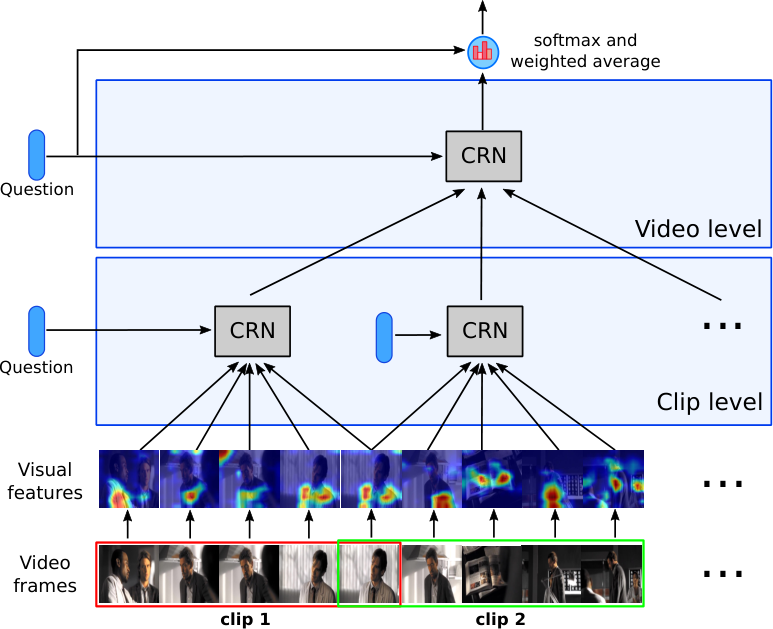
5.3.3 Answer Decoders

Similar to Sec. 4.3.4 in the previous chapter, we follow previous works (Fan et al. 2019; Jang et al. 2017; Song et al. 2018) to adopt different answer decoders depending on the task, as follows:

•

QA pairs with open-ended answers are treated as multi-class classification problems. For these, we employ a classifier which takes as input the combination of the retrieved information from visual stream $\tilde{\mathbf{o}}^{v}$ , the retrieved information from textual stream $\tilde{\mathbf{o}}^{t}$ and the question representation $\mathbf{q}$ , and computes answer probabilities $\mathbf{p}\in\mathbb{R}^{|\mathcal{\bm{A}}|}$ :

$\displaystyle\mathbf{y}$	$\displaystyle=$	$\displaystyle\text{ELU}\left(\mathbf{W}^{o}\left[\tilde{\mathbf{o}}^{v};\tilde{\mathbf{o}}^{t};\mathbf{W}^{q}\mathbf{q}+\mathbf{b}\right]+\mathbf{b}\right),$	(5.19)
$\displaystyle\mathbf{y}^{\prime}$	$\displaystyle=$	$\displaystyle\text{ELU}\left(\mathbf{W}^{y}\mathbf{y}+\mathbf{b}\right),$	(5.20)
$\displaystyle\mathbf{p}$	$\displaystyle=$	$\displaystyle\textrm{softmax}\left(\mathbf{W}^{y^{\prime}}\mathbf{y}^{\prime}+\mathbf{b}\right).$	(5.21)

•

In the case of multi-choice questions where answer choices are available, we iteratively treat each answer choice $\{\mathbf{a}_{i}\}_{i=1,...,A}$ as a query in exactly the way we handle the question. Eq. 5.17 and Eq. 5.18, therefore, take each of the answer choices’ representation $\{\mathbf{a}_{i}\}$ as a conditioning feature along with the question representation. Regarding Eq. 5.19, it is replaced by:

\displaystyle\mathbf{y}

\displaystyle=

\displaystyle\text{ELU}\left(\mathbf{W}^{o}\left[\tilde{\mathbf{o}}^{v_{\text{qa}}};\tilde{\mathbf{o}}^{t_{\text{qa}}};\mathbf{W}^{q}\mathbf{q}+\mathbf{b};\mathbf{W}^{a}\mathbf{a}+\mathbf{b}\right]+\mathbf{b}\right),

(5.22)

where $\tilde{\mathbf{o}}^{v_{\text{qa}}}$ is output of visual stream respect to queries as question and answer choices, whereas $\tilde{\mathbf{o}}^{t_{\text{qa}}}$ is output of the textual stream counterpart.

•

For short-form Video QA, we simply drop the retrieved information from textual stream $\tilde{\mathbf{o}}_{t}$ in Eq. 5.19 and Eq. 5.22. We also use the popular hinge loss as what presents in (Jang et al. 2017) for pairwise comparisons, $\text{max}\left(0,1+s^{n}-s^{p}\right)$ , between scores for incorrect $s^{n}$ and correct answers $s^{p}$ to train the network:

$\displaystyle s$ $\displaystyle=$ $\displaystyle\mathbf{W}^{y^{\prime}}\mathbf{y}^{\prime}+b,$ (5.23)

where $\mathbf{W}^{y^{\prime}}\in\mathbb{R}^{1\times d}$ is a weight matrix. Regarding long-form Video QA, we use the cross entropy as the training loss for fair comparisons with prior works.
•

For repetition count task, we use a linear regression function taking $\mathbf{y^{\prime}}$ in Eq. 5.20 as input, followed by a rounding function for integer count results. The loss for this task is Mean Squared Error (MSE).

5.3.4 Complexity Analysis

We now provide a theoretical analysis of running time for CRN units and HCRN. We will show that adding layers saves computation time, just providing a justification for deep hierarchy.

5.3.4.1 CRN Units

For clarity, let us recall the notations introduced in our CRN units: $k_{\text{max}}$ is maximum subset (also tuple) size considered from a given input array of $n$ objects, subject to $k_{\text{max}}<n$ ; $t$ is number of size- $k$ subsets, ( $k=2,3,...,k_{\text{max}}$ ), randomly sampled from the input set; $g^{k}(.),h^{k}(.,.)$ and $p^{k}(.)$ are sub-networks for relation modelling, conditioning and aggregating, respectively. In our implementation, $g^{k}(.)$ and $p^{k}(.)$ are chosen to be set functions and $h^{k}(.,.)$ is a nonlinear transformation that fuses modalities.

Each input object in CRN is arranged into a matrix of size $K\times F$ , where $K$ is the number of object elements and $F$ is the embedding size for each element. All the operations involving input objects are element-wise, that is, they are linear in time w.r.t. $K$ . Assume that the set function of order $k$ in the CRN’s operation in Alg. 1 has linear time complexity in $k$ . This holds true for most aggregation functions such as mean, max, sum or product. With the relation orders ranging from $k=2,3,...,k_{\text{max}}$ and sampling frequency $t$ , inference cost in time for a CRN is:

\displaystyle\text{cost}_{CRN}\left(t,k_{\text{max}},K,F\right)

\displaystyle=

\displaystyle\text{cost}(g)+\text{cost}(h),

(5.24)

where,

	$\displaystyle\text{cost}(g)$	$\displaystyle=$	$\displaystyle\mathcal{O}\left(\frac{t}{2}k_{\text{max}}(k_{\text{max}}-1)KF\right),$
	$\displaystyle\text{cost}(h)$	$\displaystyle=$	$\displaystyle\mathcal{O}\left((4t+2)(k_{max}-1)KF^{2}\right).$

Here the running time of $\text{cost}(g)$ is quadratic in length because each $g(.)$ that takes $k$ objects as input will cost $k$ time, for $k=2,3,...,k_{\text{max}}$ . The running time of $\text{cost}(g)$ is quadratic in $F$ due to the feature transformation operation that costs $F^{2}$ time. When $k_{\text{max}}\ll F$ , $\text{cost}(h)$ will dominate the time complexity. However, since the function $h(.)$ involves matrix operations only, it is usually fast.

The unit produces an output array of length $k_{max}-1$ , where each output object is of the same size as the input objects.

5.3.4.2 HCRN Models

We adhere to the complexity analysis of visual stream only which increases linearly in complexity with a video length. The overall complexity of HCRN depends on the design choice for each CRN unit and the specific arrangement of CRN units. For clarity, let $t=2$ and $k_{\max}=n-1$ , which are found to work well in experiments. Let $L$ be the video length, organised into $N$ clips of length $T$ each, i.e., $L=NT$ .

2-level HCRN:

Consider, for example, the 2-level architecture HCRN, representing clips and video. Each level is a stack of two CRN layers, one for motion conditioning followed by the other for linguistic conditioning. The clip-level CRNs cost $N\times\text{cost}_{CRN}\left(2,T-1,1,F\right)$ time for motion conditioning and $N\times\text{cost}_{CRN}\left(2,T-3,1,F\right)$ time for question conditioning, where $\text{cost}_{CRN}$ is the cost estimator in Eq. (5.24). This adds to roughly $\mathcal{O}\left(2TLF\right)+\mathcal{O}\left(10LF^{2}\right)$ time.

Now the output array of size $(T-4)\times F$ for the question-conditioned clip-level CRN becomes one in $N$ input objects the video-level CRNs. The CRNs at the video level, therefore, take a cost of $\text{cost}_{CRN}\left(2,N-1,T-4,F\right)$ time for the motion-conditioned one and $\text{cost}_{CRN}\left(2,N-3,T-4,F\right)$ time for the question-conditioned one, respectively, totalling $\mathcal{O}\left(2NLF\right)+\mathcal{O}\left(10LF^{2}\right)$ in order. Here we have made use of the identity $L=NT$ . The total cost is therefore in the order of $\mathcal{O}\left(2(T+N)LF\right)+\mathcal{O}\left(20LF^{2}\right)$ .

3-level HCRN:

Let us now analyse a 3-level architecture HCRN that generalises the 2-level HCRN. The $N$ clips are organised into $P$ sub-videos, each has $Q$ clips, i.e., $N=PQ$ . Since the CRNs at clip level remain the same, the first level costs $2TLF$ time to compute as before. Moving to the next level, each sub-video CRN takes as input an array of length $Q$ , whose elements have size $(T-4)\times F$ . Applying the same logic as before, the set of sub-video-level CRNs cost roughly $P\times\text{cost}_{CRN}\left(2,Q-1,T-4,F\right)$ time or approximately $\mathcal{O}\left(2\frac{N}{P}LF\right)+\mathcal{O}\left(10LF^{2}\right)$ . Here we have used the identities $N=PQ$ and $L=NT$ .

A stack of two sub-video CRNs now produces an output array of size $(Q-4)(T-4)\times F$ , serving as an input object in an array of length $P$ for the video-level CRNs. Thus the video-level CRNs cost roughly

\displaystyle\text{cost}_{CRN}\left(2,P-1,(Q-4)(T-4),F\right)

time or approximately $\mathcal{O}\left(2PLF\right)+\mathcal{O}\left(10LF^{2}\right)$ . Here we again have used the identities $L=NT$ and $N=PQ$ . Thus the total cost is in the order of $\mathcal{O}\left(2(T+\frac{N}{P}+P)LF\right)+\mathcal{O}\left(30LF^{2}\right)$ .

Deeper models might save time for long videos:

Recall that the 2-level HCRN has time cost of

\displaystyle\mathcal{O}\left(2(T+N)LF\right)+\mathcal{O}\left(20LF^{2}\right),

and the 3-level HCRN the cost of

\displaystyle\mathcal{O}\left(2(T+\frac{N}{P}+P)LF\right)+\mathcal{O}\left(30LF^{2}\right).

Here the cost that is linear in $F$ is due to the $g$ functions, and the quadratic cost in $F$ is due to the $h$ functions.

When going from 2-level to 3-level architectures, the cost for the $g$ functions drops by $\mathcal{O}\left(2(N-\frac{N}{P}-P)LF\right)$ , and the cost for the $h$ functions increases by $\mathcal{O}\left(10LF^{2}\right)$ . Now assuming $N\gg\max\left\{P,\frac{N}{P}\right\}$ , for example $P\approx\sqrt{N}$ and the number of clips $N>20$ . Then the linear drop can be approximated further as $\mathcal{O}\left(2NLF\right)$ . As $N=\frac{L}{T}$ , this can be written as $\mathcal{O}\left(2\frac{L^{2}}{T}F\right)$ . In practice the clip size $T$ is often fixed, thus the drop in the $g$ functions scales quadratically with video length $L$ , whereas the increase in the $h$ functions scales linearly with $L$ . This suggests that going deeper in hierarchy could actually save the running time for long videos.

See Subsec. 5.4.4.3 for empirical validation of the saving.

5.4 Experiments

5.4.1 Datasets

We evaluate the effectiveness of the proposed CRN unit and the HCRN architecture on a series of short-form and long-form Video QA datasets. In particular, we use three different datasets as benchmarks for the short-form Video QA, namely TGIF-QA (Jang et al. 2017), MSVD-QA (Xu et al. 2017b) and MSRVTT-QA (Xu et al. 2016). All those three datasets are collected from real-world videos. We also evaluate HCRN on long-form Video QA using one of the largest datasets publicly available, TVQA (Lei et al. 2018). Details of each benchmark are as below.

TGIF-QA:

This is currently the most prominent dataset for Video QA, containing 165K QA pairs and 72K animated GIFs. The dataset covers four tasks addressing the unique properties of video data. Of which, the first three require strong spatio-temporal reasoning abilities: Repetition Count - to retrieve the number of occurrences of an action, Repeating Action - multi-choice task to identify the action that is repeated for a given number of times, State Transition - multi-choice tasks regarding temporal order of events. The last task - Frame QA - is akin to image QA where the answer to a given question can be found from one particular video frame. Please see Sec. 4.4.1 for more details of the TGIF-QA dataset.

MSVD-QA:

This is a small dataset of 50,505 question answer pairs annotated from 1,970 short clips. Questions are of five types, including what, who, how, when and where, of which 61% of questions are used for training whilst 13% and 26% are used as the validation set and test set, respectively.

MSRVTT-QA:

The dataset contains 10K videos and 243K question answer pairs. Similar to MSVD-QA, questions are of five types. Splits for train, validation and test are with the proportions are 65%, 5%, and 30%, respectively. Compared to the other two datasets, videos in MSRVTT-QA contain more complex scenes. They are also much longer, ranging from 10 to 30 seconds long, equivalent to 300 to 900 frames per video.

TVQA:

This is one of the largest long-form Video QA datasets annotated from 6 different TV shows: The Big Bang Theory, How I Met Your Mother, Friends, Grey’s Anatomy, House, Castle. There are total 152.5K question-answer pairs associated with 5 answer choices each from 21,8K long clips of 60/90 secs which comes down to 122K, 15,25K and 15,25K for train, validation and test set, respectively. The dataset also provides start and end timestamps for each question to limit the video portion where one can find corresponding answers.

Regarding the evaluation metric, we mainly use accuracy in all experiments, excluding those for repetition count on TGIF-QA dataset where Mean Square Error (MSE) is used.

5.4.2 Implementation Details

5.4.2.1 Feature Extraction

For short-form Video QA datasets, each video is preprocessed into $N$ short clips of fixed lengths, 16 frames each. In detail, we first locate $N$ equally spaced anchor frames. Each clip is then defined as a sequence of 16 consecutive video frames taking a pre-computed anchor as the middle frame. For the first and the last clip where frame indices may exceed the boundaries, we repeat the first frame or the last frame of the video multiple times until it fills up the clip’s size.

Given segmented clips, we extract motion features for each clip using a pre-trained model of the ResNeXt-101¹¹ 1 https://github.com/kenshohara/video-classification-3d-cnn-pytorch (Xie et al. 2017; Hara et al. 2018). Regarding the appearance feature used in the experiments, we take the pool5 output of ResNet (He et al. 2016) features as a feature representation of each frame. This means we completely ignore the 2D structure of spatial information of video frames which is likely to be beneficial for answering questions particularly interested in object’s appearance, such as those in the Frame QA task in the TGIF-QA dataset. We are aware of this but deliberately opt for light-weighted extracted features, and drive the main focus of this chapter on the significance of temporal relation, motion, and the hierarchy of video data by nature. Note that most of the videos in the datasets in the short-form Video QA category, except those in the MSRVTT-QA dataset, are short. Hence, we intentionally divide each video into 8 clips (8 $\times$ 16 frames) to produce partially overlapping frames between clips to avoid temporal discontinuity. Longer videos in MSRVTT-QA are additionally segmented into 24 clips of 16 frames each, primarily aiming at evaluating the model’s ability to handle very long sequences.

For the TVQA long-form dataset, we did a similar strategy as for short-video where we divide each video into $N$ clips. However, as TVQA videos are longer and only recorded at 3fps, we adapt by choosing $N=6$ , each clip contains 8 frames based on empirical experiences. The pool5 output of ResNet features is also used as the feature representation of each frame.

For the subtitles, the maximum subtitle’s length is set at $256$ . We simply cut off those who are longer than that and do zero paddings for those who are shorter. Subtitles are further divided into 6 segments overlapping at half a segment size.

5.4.2.2 Network Training

HCRN and its variations are implemented in Python 3.6 with Pytorch 1.2.0. Common settings include $d=512$ , $t=2$ for both visual and textual streams. For all experiments, we train the model using Adam optimiser with a batch size of 32 , initially at a learning rate of $10^{-4}$ and decay by half after every 5 epochs for counting task in the TGIF-QA dataset and after every 10 epochs for the others. All experiments are terminated after 25 epochs and reported results are at the epoch giving the best validation accuracy. Depending on the amount of training data and hierarchy depth, it may take around 4-30 hours of training on one single NVIDIA Tesla V100 GPU. Pytorch implementation of the model is publicly available. ²² 2 https://github.com/thaolmk54/hcrn-videoqa.

As for experiments with the large-scale language representation model BERT, we use the latest pre-trained model provided by Hugging Face³³ 3 https://github.com/huggingface/transformers. We fine-tune the BERT model during training with a learning rate of $2\times 10^{-5}$ in all experiments.

5.4.3 Quantitative Results

We compare our proposed model with state-of-the-art methods (SOTAs) on the aforementioned datasets. By default, we use pre-trained GloVe embedding (Pennington et al. 2014) for word embedding following by a BiLSTM for sequential modelling. Experiments using contextual embeddings by a pre-trained BERT network (Devlin et al. 2019) is explicitly specified with “(BERT)”. Detailed experiments for short-form Video QA and long-form Video QA are as the following.

5.4.3.1 Short-form Video QA

For TGIF-QA, we compare with most recent SOTAs, including (Fan et al. 2019; Gao et al. 2018; Jang et al. 2017; Li et al. 2019c), over four tasks. These works, except for (Li et al. 2019c), make use of motion features extracted from either optical flow or 3D CNNs and its variants.

The results are summarised in Table 5.2 for TGIF-QA, and in Fig. 5.8 for MSVD-QA and MSRVTT-QA. Results of the previous works are taken from either the original papers or what reported by Fan et al. 2019. It is clear that our model consistently outperforms or achieves competitive performance with the SOTA models on all tasks across all datasets. The improvements are particularly noticeable when strong temporal reasoning is required, i.e., for the questions involving actions and transitions in TGIF-QA. These results confirm the significance of the modelling of both near-term and far-term temporal relations toward finding correct answers. In addition, results on the TGIF-QA dataset over 10 runs of different random seeds confirm the robustness of the CRN units against the randomness in input subsets selection. More analysis on how relations affect the model’s performance is provided in later ablation studies.

Regarding results with the recent advance in language representation model BERT, it does not have much effect on the results across tasks requiring strong temporal reasoning in the TGIF-QA. This can be explained by the fact that questions in this dataset are relatively short and all questions are created from a limited number of patterns, hence, contextual embeddings do not account much benefit. Whereas the Frame QA task relies on much richer vocabulary, thanks to its free-form questions, hence, contextual embeddings extracted by BERT greatly boost the model’s performance on this task. We also empirically find out that fine-tune only the last two layers of the BERT network gives more favourable performance comparing to fine-tuning all layers.

The MSVD-QA and MSRVTT-QA datasets represent highly challenging benchmarks for machine compared to the TGIF-QA, thanks to their open-ended nature. Our model HCRN outperforms existing methods on both datasets, achieving 36.8% and 35.4% accuracy which are 2.4 points and 0.4 points improvement on MSVD-QA and MSRVTT-QA, respectively. This suggests that the model can handle both small and large datasets better than existing methods. We also fine-tune the contextual embeddings by BERT on these two datasets. Results show that the contextual embeddings bring great benefits on both MSVD-QA and MSRVTT-QA, achieving 39.3% and 38.3% accuracy, respectively. These figures are consistent with the result on the Frame QA task of the TGIF-QA dataset. Please note that we also fine-tune only last two layers of the BERT network in these experiments simply due to favourable empirical results.

Finally, we provide a justification for the competitive performance of our HCRN against existing rivals by comparing model features in Table 5.3. Whilst it is not straightforward to compare head-to-head on internal model designs, it is evident that effective video modelling necessitates handling of motion, temporal relation and hierarchy at the same time. We will back this hypothesis by further detailed studies in Sec. 5.4.4 (for motion, temporal relations, shallow hierarchy) and Subsec. 5.4.4.3 (deep hierarchy).

5.4.3.2 Long-form Video QA

For TVQA, we compare our method to several baselines and recent state-of-the-art methods (See Table 5.4). The dataset is relatively new, and due to the challenges with long-form Video QA, there are only several attempts in benchmarking it. Comparisons of the proposed method with the baselines and other methods are made on the validation set. Results of compared methods are taken as reported in their original publications. Experiments using timestamp information are indicated by w/ ts and those with full-length subtitles are with w/o ts. If not indicated explicitly, “V.”, “S.”, “Q.” short for visual features, subtitle features and question features, respectively. The evaluated settings are as follows:

•

(B) Q. : This is the simplest baseline where we only use question features for predicting the correct answer. Results in this setting will reveal how much our model relies on the linguistic bias to arrive at correct answers.
•

(B) S. + Q. (w/o pre-selection): In this baseline, we use question and subtitle features for prediction. Both question and subtitle features are simply obtained by concatenating the final output hidden states of forward and backward LSTM passes and further pass to a classifier as in Sec. 5.3.3.
•

(B) S. + Q. (w/ pre-selection): This baseline is to show the significance of pre-selection in the textual stream as in Eq. 5.18. Question features and selective output between the question and the subtitles as explained in Eq. 5.18 are fed into a classifier for prediction.
•

(B) V. + Q.: In this baseline, we simply apply average pooling to squeeze the visual features of entire videos into a vector and further combine it with question features for prediction.
•

(B) S. + V. + Q. (w/ pre-selection): We combine two baselines “(B) S. + Q. (w/ pre-selection)” and “(B) V. + Q.” right above. Given that, subtitle features are extracted with pre-selection as in Eq. 5.18 and video features are smashed over space-time before going through a classifier.
•

(HCRN) S. + Q.: This is to evaluate the effect of the textual stream alone in our proposed network architecture as described in Fig. 5.6.
•

(HCRN) V. + Q.: This is to evaluate the effect of the visual stream counterpart alone in Fig. 5.7.
•

(HCRN) S. + V. + Q.: Our full proposed architecture with the presence of both two modalities.

As shown in Table 5.4, using BERT for contextual word embeddings significantly improves performance comparing to GloVe embeddings and BiLSTM counterpart. The results are consistent with what reported by Yang et al. 2020. Although our model only achieves competitive performance with Yang et al. 2020 in the setting of using timestamps (71.3 vs. 72.1), we significantly outperform them by 3.0 absolute points on the more challenging setting when we do not have access to timestamp indicators of where answers located. This clearly shows that our bottom-up approach is promising to solve long-form Video QA in its general setting.

Even though BERT is designed to do contextual embedding which pre-computes some word relations, HCRN still shows additional benefit in modelling relations between segments in the passage. However, this benefit is not as clearly demonstrated as in the case of using GloVe embedding coupled with BiLSTM (Table 5.4 - Exp. 9 vs. Exp. 7 and Exp. 13 vs. Exp. 14). To deeper understanding the behaviour of HCRN, we will concentrate our further analysis using comparison with GloVe + LSTM.

It clearly shows that using output hidden states of BiLSTM to represent subtitle features directly for classification has a very limited effect (See Table 5.4 - Exp. 3 vs Exp. 4). The results could be explained as LSTM fails to handle such long subtitles of hundreds of words. In the meantime, pre-selection plays a critical role to find relevant information in the subtitles to a question which boosts performance from 42.3% to 57.9% when using full subtitles and from 41.8% to 62.1% when using timestamps (See Exp. 5). Our HCRN further improves approximately 1.0 points (without timestamp annotation) and 1.5 points (with timestamp annotation) comparing to the baseline of GloVe embeddings and BiLSTM with pre-selection for the textual stream only setting. As for the effects on visual stream, our HCRN gains around 1.0 points over the baseline of averaging visual features. This leads to an improvement of north of 1.0 points when leveraging both visual and textual stream together (See Exp. 12 vs. Exp. 15) on both settings with timestamp annotation and without timestamp annotation. Even though our results are behind the method developed by Lei et al. 2018, we wish to point out that their context matching model with the bi-directional attention flow (BiDAF) (Seo et al. 2017) significantly contributes to the performance. Whereas, our model only makes use of vanilla BiLSTM to sequence modelling. Therefore, a direct comparison between the two methods is unfair. We instead mainly compare our method with a simple variant of Lei et al. 2018 by dropping off the BiDAF to show the contribution of our CRN unit as well as the HCRN network. This is equivalent to the baseline (B) S. + V. + Q. (w/ pre-selection) in this thesis.

Model	Action	Trans.	Frame	Count
ST-TP (Jang et al. 2017)	62.9	69.4	49.5	4.32
Co-mem (Gao et al. 2018)	68.2	74.3	51.5	4.10
PSAC (Li et al. 2019c)	70.4	76.9	55.7	4.27
HME (Fan et al. 2019)	73.9	77.8	53.8	4.02
HCRN*	75.2 $\pm$ 0.4	81.3 $\pm$ 0.2	55.9 $\pm$ 0.3	3.93 $\pm$ 0.03
HCRN (embeddings with BERT)	69.8	79.8	57.9	3.96

Table 5.2: Comparison with the state-of-the-art methods on TGIF-QA dataset. For count, the lower the better (MSE) and the higher the better for the others (accuracy). *Means with standard deviations over 10 runs.

Figure 5.8: Performance comparison on MSVD-QA and MSRVTT-QA dataset with state-of-the-art methods: Co-mem (Gao et al. 2018), HME (Fan et al. 2019), HRA (Chowdhury et al. 2018), and AMU (Xu et al. 2017b).

Model	Appearance	Motion	Hierarchy	Relation
ST-TP (Jang et al. 2017)	$\checkmark$	$\checkmark$
Co-mem (Gao et al. 2018)	$\checkmark$	$\checkmark$
PSAC (Li et al. 2019c)	$\checkmark$
HME (Fan et al. 2019)	$\checkmark$	$\checkmark$
HCRN	$\checkmark$	$\checkmark$	$\checkmark$	$\checkmark$

Table 5.3: Model design choices and input modalities in comparison. See Table 5.2 for corresponding performance on TGIF-QA dataset.

Exp.	Model	Val. Acc.
Exp.	Model	w/o ts	w/ ts
	State-of-the-art methods
1	TVQA S.+Q.+V. (Lei et al. 2018; Yang et al. 2020)	64.7	67.7
2	VideoQABERT (Yang et al. 2020)	63.1	72.1
	Textual stream only
3	(B) Q.	41.6	41.6
4	(B) S. + Q. (w/o pre-selection)	42.3	41.8
5	(B) S. + Q. (w/ pre-selection)	57.9	62.1
6	(B) Q. (BERT)	44.2	44.2
7	(B) S. + Q. (BERT)	65.1	71.1
8	(HCRN) S. + Q.	59.0	63.6
9	(HCRN) S. + Q. (BERT)	66.0	71.1
	Visual stream only
10	(B) V. + Q.	42.2	42.2
11	(HCRN) V. + Q.	43.1	43.1
	Two streams
12	(B) S. + V. + Q. (w/ pre-selection)	58.5	63.2
13	(B) S. + V. + Q. (BERT)	65.7	71.4
14	(HCRN) S. + V. + Q. (BERT)	66.1	71.3
15	(HCRN) S. + V. + Q.	59.1	64.7

Table 5.4: Comparison with baselines and state-of-the-art methods on TVQA dataset. w/o ts: without using timestamp annotation to limit the search space of where to find answers; w/ ts: making use of the timestamp annotation.

5.4.4 Ablation Studies

Model	Action	Transition	FrameQA	Count
Relations $(k_{max},t)$
$k_{max}=1,t=1$	72.8	80.7	56.3	3.87
$k_{max}=1,t=3$	73.4	81.1	56.0	3.94
$k_{max}=1,t=5$	74.0	80.3	56.4	3.86
$k_{max}=1,t=7$	74.8	80.0	56.5	3.85
$k_{max}=1,t=9$	73.7	81.1	56.4	3.82
$k_{max}=2,t=2$	72.8	80.8	56.3	3.80
$k_{max}=2,t=9$	73.1	81.4	56.0	3.85
$k_{max}=4,t=2$	74.2	81.5	56.8	3.88
$k_{max}=4,t=9$	73.4	81.8	56.5	3.83
$k_{max}=\left\lfloor n/2\right\rfloor,t=2$	74.7	81.1	55.7	3.85
$k_{max}=\left\lfloor n/2\right\rfloor,t=9$	74.7	81.0	55.4	3.94
$k_{max}=n-1,t=1$	74.2	80.8	55.3	3.98
$k_{max}=n-1,t=3$	75.2	81.1	56.2	4.00
$k_{max}=n-1,t=5$	75.0	81.3	55.6	3.95
$k_{max}=n-1,t=7$	75.3	81.9	55.8	4.00
$k_{max}=n-1,t=9$	74.9	81.1	55.6	3.94
Fix $k=k_{max},k_{max}=n-1,t=2$	72.9	80.2	56.5	3.90
Hierarchy
$1$ -level, video CRN only	72.7	81.4	57.2	3.88
$1.5$ -level, clips $\rightarrow$ pool	73.1	81.2	57.2	3.88
Motion conditioning
w/o motion	69.8	78.4	57.9	4.38
w/o short-term motion	74.1	80.9	56.4	3.87
w/o long-term motion	75.8	80.8	56.8	3.97
Linguistic conditioning
w/o linguistic condition	68.7	80.5	56.6	3.92
w/o question at the clip level	75.0	81.0	56.0	3.85
w/o question at the video level	74.2	81.0	55.3	3.90
Multiplicative relation
w/o MUL. in all CRNs	74.0	81.7	55.8	3.86
w/ MUL. for both question and motion	75.4	80.2	55.1	3.98
Subset sampling
Sampled from pre-computed superset	75.2	81.3	55.9	3.90
Directly sampled	75.3	81.8	55.3	3.89

Table 5.5: Ablation studies on TGIF-QA dataset. For count, the lower the better (MSE) and the higher the better for the others (accuracy). When not explicitly specified, we use

k_{max}=n-1,t=2

for relation order and sampling resolution.

Exp.	Model	Val. Acc.
Exp.	Model	w/o ts	w/ ts
	Textual stream only
1	S. + Q. (w/ MUL. + w/ LSTM)	59.0	63.6
2	S. + Q. (w/ MUL. + w/o LSTM)	57.1	63.6
3	S. + Q. (w/o MUL. + w/ LSTM)	59.1	63.9
4	S. + Q. (w/o MUL. + w/o LSTM)	57.4	63.5
	Visual stream only
5	V. + Q. (w/ MUL. + w/ LSTM)	42.7	42.7
6	V. + Q. (w/ MUL. + w/o LSTM)	43.1	43.1
7	V. + Q. (w/o MUL. + w/ LSTM)	42.2	42.2
8	V. + Q. (w/o MUL. + w/o LSTM)	42.1	42.1
	Two streams
9	S. + V. + Q. (S. w/ MUL. + LSTM, V. w/ MUL.)	59.1	64.7

Table 5.6: Ablation studies on TVQA dataset.

To provide more insights about the roles of CRN’s components, we conduct extensive ablation studies on the TGIF-QA and TVQA dataset with a wide range of configurations. The results are reported in Table 5.5 for the short-form Video QA and in Table 5.6 for the long-form Video QA.

5.4.4.1 Short-form Video QA

Overall, we find that our sampling method does not hurt the HCRN performance that much while it is much more effective than the one used by Zhou et al. 2018 in terms of complexity. We also find that ablating any of the design components or CRN units would degrade the performance for temporal reasoning tasks (actions, transition and action counting). The effects are detailed as follows.

Effect of relation order $k_{max}$ and resolution $t$ :

Without relations ( $k_{max}=1,t=1$ ) the performance suffers, specifically on actions and events reasoning whereas counting tends to be better. This is expected since those questions often require putting actions and events in relation with a larger context (e.g., what happens before something else) while motion flow is critical for counting but for far-term relations. In this case, most of the tasks benefit from increasing sampling resolution $t$ $(t>1)$ because of better chance to find a relevant frame as well as the benefits of the far-term temporal relation learned by the aggregating sub-network $p^{k}(.)$ of the CRN unit. However, when taking relations into account ( $k_{max}>1$ ), we find that HCRN is robust against sampling resolution $t$ but depends critically on the maximum relation order $k_{max}$ . The relative independence w.r.t. $t$ can be due to visual redundancy between frames, so that resampling may capture almost the same information. On the other hand, when considering only low-order object relations, the performance is significantly dropped in action and transition tasks while it is slightly better for counting and frame QA. These results confirm that high-order relations are required for temporal reasoning. As the frame QA task requires only reasoning on a single frame, incorporating temporal information might confuse the model. Similarly, when the model only makes use of the high-order relations (Fix $k=k_{max},k_{max}=n-1,t=2$ ), the performance suffers, suggesting combining both low-order object relations and high-order object relations is a lot more efficient.

Effect of hierarchy:

We design two simpler models with only one CRN layer:

•

$1$ -level, $1$ CRN video on key frames only: Using only one CRN at the video-level whose input array consists of key frames of the clips. Note that video-level motion features are still maintained.
•

$1.5$ -level, clip CRNs $\rightarrow$ pooling: Only the clip-level CRNs are used, and their outputs are mean-pooled to represent a given video. The pooling operation represents a simplistic relational operation across clips. The results confirm that a hierarchy is needed for high performance on temporal reasoning tasks.

Effect of motion conditioning:

We evaluate the following settings:

•

w/o short-term motions: Remove all CRN units that condition on the short-term motion features (clip level) in the HCRN.
•

w/o long-term motions: Remove the CRN unit that conditions on the long-term motion features (video level) in the HCRN.
•

w/o motions: Remove motion feature from being used by HCRN. We find that motion, in agreeing with prior arts, is critical to detect actions, hence computing action count. Long-term motion is particularly significant for the counting task, as this task requires maintaining a global temporal context during the entire process. For other tasks, short-term motion is usually sufficient. E.g. in the action task, wherein one action is repeatedly performed during the entire video, long-term context contributes little. Not surprisingly, motion does not play a positive role in answering questions on single frames as only appearance information needed.

Effect of linguistic conditioning and multiplicative relation:

Linguistic cues represent a crucial context for selecting relevant visual artefacts. For that we test the following ablations:

•

w/o question at the clip level: Remove the CRN unit that conditions on question representation at clip level.
•

w/o question at the video level: Remove the CRN unit that conditions on question representation at video level.
•

w/o linguistic condition: Exclude all CRN units conditioning on linguistic cue while the linguistic cue is still in the answer decoder. Likewise, the multiplicative relation form offers a selection mechanism. Thus we study its effect as follows:
•

w/o MUL. in all CRNs: Exclude the use of multiplicative relations in all CRN units.
•

w/ MUL. relation for question and motion: Leverage multiplicative relations in all CRN units.

We find that the conditioning question provides an important context for encoding video. Conditioning features (motion and language), through the multiplicative relation as in Eq. 5.3, offers further performance gain in all tasks rather than Frame QA, possibly by selectively passing question-relevant information up the inference chain.

Effect of subset sampling

We conduct experiments with the full model of Fig. 5.5 (a) with $k_{max}=n-1,t=2$ . The experiment “Sampled from pre-computed superset” refers to our CRN units of using the same sampling trick as what is in (Zhou et al. 2018), where the set $\mathbf{Q}^{k}$ is sampled from a pre-computed collection of all possible size- $k$ subsets. “Directly sampled”, in contrast, refers to our sampling method as described in Alg. 1. The empirical results show that directly sampling size- $k$ subsets from an input set does not degrade much of the performance of the HCRN for short-form Video QA, suggesting it a better choice when dealing with large input sets in size to reduce the complexity of the CRN units.

5.4.4.2 Long-form Video QA

We focus on studying the effect of different options for the conditioning sub-network $h^{k}(.,.)$ in Sec. 5.3.1 which reflects the flexibility of our model when dealing with different forms of input modalities. The options are:

•

S. + Q. (w/ MUL. + w/ LSTM): Only textual stream is used. The conditioning sub-network $h^{k}(.,.)$ is with multiplicative relation between tuples of segments and conditioning feature, and coupled with BiLSTM as formulated in Eqs. (5.4, 5.5 and 5.6).
•

S. + Q. (w/ MUL. + w/o LSTM): Remove the BiLSTM network in the experiment S. + Q. (w/ MUL. + w/ LSTM) to evaluate the effect of sequential modelling in textual stream.
•

S. + Q. (w/o MUL. + w/ LSTM): The multiplicative relation in the experiment S. + Q. (w/ MUL. + w/ LSTM) is now replaced with a simple concatenation of conditioning feature and tuples of segments.
•

S. + Q. (w/o MUL. + w/o LSTM): Remove the BiLSTM network in the right above experiment S. + Q. (w/o MUL. + w/ LSTM) to evaluate the effect of when both selective relation and sequential modelling are missing.
•

V. + Q. (w/ MUL. + w/ LSTM): Only visual stream is under consideration. We use the multiplicative form as in Eq. 5.3 for the conditioning sub-network instead of a simple concatenation operation in Eq. 5.2. We additionally use a BiLSTM network for sequential modelling as same as the way we have done with the textual stream. This is because both visual content and textual content are temporal sequences by nature.
•

V. + Q. (w/ MUL. + w/o LSTM): Similar to the above experiment V. + Q. (w/ MUL. + w/ LSTM) but without the use of the BiLSTM network.
•

V. + Q. (w/o MUL. + w/ LSTM): The conditioning sub-network is simply a tensor concatenation operation. This is to compare against the one using multiplicative form V. + Q. (w/ MUL. + w/ LSTM).
•

V. + Q. (w/o MUL. + w/o LSTM): Similar to V. + Q. (w/o MUL. + w/ LSTM) but without the use of the BiLSTM network for sequential modelling.
•

S. + V. + Q. (S. w/ MUL. + LSTM, V. w/ MUL.): Both two streams are present for prediction. We combine the best option of each network stream, S. + Q. (w/ MUL. + w/ LSTM) for the textual stream and V. + Q. (w/ MUL. + w/o LSTM) for the visual stream for comparison.

It is empirically shown that the simple concatenation as in Eq. 5.2 is insufficient to combine conditioning features and output of relation network in this dataset. In the meantime, the multiplicative relation between the conditioning features and those relations is a better fit as it greatly improves the model’s performance, especially in the visual stream. This shows the consistency in empirical results between long-form Video QA and shot-form Video QA where the relation between visual content and the query is more about multiplicative (selection) rather than simple additive.

On the other side, sequential modelling with BiLSTM is more favourable for textual stream than visual stream even though both streams are sequential by nature. This well aligns with our analysis in Sec. 5.3.1.

Depth of hierarchy	Overall Acc.
Depth of hierarchy	val.	test
$2$ -level, $24$ clips $\rightarrow$ $1$ vid	35.4	35.5
$3$ -level, $24$ clips $\rightarrow$ $4$ sub-vids $\rightarrow$ $1$ vid	35.1	35.4

Table 5.7: Results for going deeper hierarchy on MSRVTT-QA dataset. Run time is reduced by factor of

4

for going from 2-level to 3-level hierarchy.

5.4.4.3 Deepening Model Hierarchy Saves Time

We test the scalability of the HCRN on long videos in the MSRVTT-QA dataset, which are organised into 24 clips (3 times longer than the other two datasets). We consider two settings:

•

$2$ -level hierarchy, $24$ clips $\rightarrow$ $1$ vid: The model is as illustrated in Fig. 5.5, where 24 clip-level CRNs are followed by a video-level CRN.
•

$3$ -level hierarchy, $24$ clips $\rightarrow$ $4$ sub-vids $\rightarrow$ $1$ vid: Starting from the 24 clips as in the $2$ -level hierarchy, we group 24 clips into 4 sub-videos, each is a group of 6 consecutive clips, resulting in a $3$ -level hierarchy. These two models are designed to have a similar number of parameters, approx. 44M.

The results are reported in Table 5.7. Unlike existing methods which usually struggle with handling long videos, our method is scalable for them by offering deeper hierarchy, as analysed theoretically in Sec. 5.3.4. The theory suggests that using a deeper hierarchy can reduce the training time and inference time for HCRN when the video is long. This is validated in our experiments, where we achieve 4 times reduction in training and inference time by going from 2-level HCRN to 3-level counterpart whilst maintaining competitive performance.

5.5 Discussion

HCRN presents a new class of neural architectures for multimodal Video QA, pursuing the ease of model construction through reusable uniform building blocks. Different from temporal attention based approaches, which put effort into selecting objects, HCRN concentrates on modelling relations and hierarchy in different input modalities in Video QA. In the scope of this chapter, we study how to deal with visual content and subtitles where applicable. The visual and text streams share a similar structure in terms of near-term, far-term relations and information hierarchy. The difference in methodology and design choices between ours and the existing works leads to distinctive benefits in different scenarios as empirically proven.

Within the scope of this chapter, we did not consider the audio channel and early fusion between modalities, leaving these open for future work. Since the CRN is generic, we envision a design for the HCRN for the audio stream similar to the visual stream. The modalities can be combined at any hierarchical level, or any step within the same level. For example, as the audio, subtitle and visual content are partly synchronised, we can use a sub-HCRN to represent the three streams per segment. Alternatively, we can fuse the modalities into the same CRN as long as the feature representations are projected onto the same tensor space. Future works will also include object-oriented representation of videos as these are native to our CRN unit, thanks to its generality. As the CRN is a relational model, both cross-object relations and cross-time relations can be modelled. These are likely to improve the interpretability of the model and get closer to how human reasons across multiple modalities. CRN units can be further augmented with attention mechanisms to cover better object selection ability, so that related tasks such as frame QA in the TGIF-QA dataset can be further improved.

5.6 Closing Remarks

We introduced a general-purpose neural unit called Conditional Relation Network (CRN) and a method to construct hierarchical networks for multimodal Video QA using the CRN as a building block. The CRN is a relational transformer that encapsulates and maps an array of tensorial objects into a new array of relations, all conditioned on a contextual feature. In the process, high-order relations among input objects are encoded and modulated by a conditioning feature. This design allows flexible construction of sophisticated structures such as stacking and hierarchy and supports iterative reasoning, making it suitable for QA over multimodal inputs and structured domains like video. The HCRN was evaluated on multiple Video QA datasets, covering both short-form Video QA whose questions are mainly about activities/events happening in a short snippet (TGIF-QA, MSVD-QA, MSRVTT-QA) and long-form Video QA whose questions are related to both long movie scenes and associated movie subtitles (TVQA dataset). HCRN demonstrates its competitive reasoning capability in a wide range of different settings against state-of-the-art methods. The examination of CRN in Video QA highlights the importance of building a generic neural reasoning unit that supports native multimodal interaction in improving robustness of visual reasoning.

Viewing our HCRN under the dual process neural architecture introduced in Chapter 4, it plays the role of System 1 with advanced visual perception by the capability to encode a wider range of information and relations needed for the reasoning process than exisiting methods including our own Clip-based Relational Network in the previous chapter. However, HCRN has not yet considered the explicit relationships between semantic objects (e.g. person, car, cat etc.). The current implementation of HCRN assumed frame features at a time step as abstract objects. The following chapter will address this issue by using the categorical and relational structures of semantic objects to advance reasoning functionalities.

Chapter 6 Relational Visual Reasoning

6.1 Introduction

Human visual reasoning involves analysing linguistic aspects of the query and continuously inter-linking them with visual objects through a series of information aggregation steps (Lake et al. 2017). Artificial reasoning engines mimic this ability by using structured representations (e.g. scene graphs) (Shi et al. 2019) to discover categorical and relational information about visual objects.

In the previous chapters, we studied the importance of reasoning for an intelligent agent by asking it to answer questions about the temporal dynamics in videos. The findings showed that temporal relations, compositionality and the hierarchical design of the models are vital for machine agents to perform visual reasoning. However, we neglect the explicit associations and interactions of cross-modality components in our models. In this chapter, we focus on exploring the significance of structured representations of inputs in visual reasoning. For simplicity, we use Image Question Answering (Image QA) as the testbed for evaluating the benefits of these structures to neural networks in learning and reasoning.

We address two key abstractions in this chapter: How can we extend structured representations of input modalities seamlessly across both visual-lingual borders? Furthermore, how can we extend these structures to be dynamic and responsive to the reasoning process rather than static representations as in prior studies? We explore the dynamic relational structures of visual scenes that are proactively discovered within reasoning context and their adaptive connections to the components of a linguistic query to answer visual questions effectively.

Recent history observes the success of compositional reasoning which iteratively pays attention to a subset of clues in the query and simultaneously looks up a corresponding subset of facts from a static unstructured knowledge source to construct a representation related to the answer (Hudson and Manning 2018). Concurrently, findings in visual relational modelling show that the information in visual scenes is significantly distributed at the interconnections between semantic factors of visual objects and linguistic objects from both the image and query (Baradel et al. 2018). These observations suggest that relational structures can improve compositional reasoning (Xu et al. 2019). However, direct application of attention mechanisms on a static structuralised knowledge source (Veličković et al. 2018) would miss the full advantage of compositionality. Moreover, object relations are naturally rich and multifaceted (Kim et al. 2018c), therefore an a priori defined set of semantic predicates such as visual scene graphs (Hudson and Manning 2019b) and language grounding (Huang et al. 2019) are either incomplete (Xu et al. 2017a), or too complicated and irrelevant to use without further pruning.

We approach this dilemma by dynamically constructing relevant object connections on-demand according to the evolving reasoning states. There are two types of connections: links that relate visual objects and links that bind visual objects in the image to linguistic counterparts in the query (See Fig. 6.1). Conceptually, this dynamic structure constitutes a relational working memory that temporarily links and refines concepts both within and across modalities. These relations are compact and readily support structural inference.

The output model in this chapter, called Language-binding Object Graph Networks (LOGNet) for Image QA, includes an iterative operation of a LOG unit that uses a contextualised co-attention to identify pairs of visual objects that are temporally related. Another co-attention head is concurrently used to provide a cross-domain binding between visual concepts and linguistic clues. A progressive chain of dynamic graphs is inferred by our model (see Fig. 6.1). These dynamic structures enable representation refinement with residual graph convolution iterations. The refined information will be added to an internal working memory progressing toward predicting the answer. The modules are interconnected through co-attention signals making the model end-to-end differentiable.

We evaluate our model on major Image QA datasets. Both qualitative and quantitative results indicate that LOGNet has advantages over state-of-the-art methods in answering long and complex questions. Our results show superior performance even when trained on just 10% of data. These questions require complex high-order reasoning which necessitates our model’s ability to dynamically couple entities to build a predicate, and then chain these predicates in the correct order. The structured representation provides guidance to the reasoning process, improving the learning fitness, particularly with limited training data.

6.2 Background

In Sec. 3.3, we have mentioned general approaches in Image QA. This section provides more background on compositional and relational reasoning, which are our main focuses. Recent compositional reasoning research aims at either structured symbolic program execution using custom-built modules (Hu et al. 2017) or working through recurrent implicit reasoning steps on an unstructured representation (Perez et al. 2018). Relational structures have been demonstrated to be crucial for reasoning (Xu et al. 2019). End-to-end relational modelling considers pair-wise predicates of CNN features (Santoro et al. 2017). With reliable object detection, visual reasoning can use semantic objects as cleaner representations (Anderson et al. 2018; Desta et al. 2018). When semantic or geometrical predicate labels are available, either as provided (Hudson and Manning 2019a) or by learning (Xu et al. 2017a) to form semantic scene graphs, such structures can be leveraged for visual reasoning (Shi et al. 2019; Li et al. 2019a).

In contrast to these methods, our relational graphs presented in this chapter are not limited by the predefined predicates but liberally form them according to the reasoning context. Our model is also different from previous question-conditioned graph construction (Norcliffe-Brown et al. 2018) in the dynamic nature of the multiform graphs where only relations that are relevant emerge. Dynamic graph modelling has been considered by recurrent modelling (Palm et al. 2018), and although their states transform, the graph structures stay fixed. A related idea uses language conditioned message passing to extract context-aware features (Hu et al. 2019). In contrast, LOGNet does not treat linguistic cues as a single conditioning vector, it instead allows them to live as a set of active objects that interact with visual objects through binding and individually contribute to the joint representation. The language binding also differentiates LOGNet from MUREL (Cadene et al. 2019) where the contributions of linguistic cues to visual objects are the same though an expensive bilinear operator.

6.3 Language-binding Object Graph Network

We formulate the Image QA task similar to the formulation of the Video QA tasks in the previous chapters. The goal of the Image QA task is to deduce an answer $\hat{y}$ in an answer space $\mathcal{\bm{A}}$ from an image $\mathcal{\bm{I}}$ in response to a natural question $\mathbf{q}$ . Mathematically, the Image QA task is presented as:

\displaystyle\hat{y}

\displaystyle=

\displaystyle\arg\max_{a\in\mathbb{\bm{\mathcal{A}}}}\mathcal{F}_{\bm{\theta}}\left(a;\mathbf{q},\mathcal{\bm{I}}\right),

(6.1)

where, $\bm{\theta}$ is the model parameters of the scoring function $\mathcal{F}\left(.\right)$ .

This chapter envisions Image QA as a process of relational reasoning over a scene of multiple visual objects conditioned on a set of linguistic cueing objects. Crucially, a pair of co-appearing visual objects may induce multiple relations, whose nature may be unknown a priori, and hence must be inferred dynamically in adaptive interaction with the linguistic cues.

We present a new neural model $\mathcal{F}\left(.\right)$ called LOGNet (See Fig. 6.2) to realise this vision. At the high level, for each image and query pair, LOGNet first normalises them into two individual sets of linguistic and visual objects. Then, it performs iterative multi-step reasoning by iteratively summoning Language-binding Object Graph (LOG) units to achieve a compact multi-modal representation in a recurrent manner. This representation is finally combined with the query representation to reach the answers. We detail these steps in Sec. 6.3.2.

6.3.1 Linguistic and Visual Objects

Similar to what presented in Sec. 3.2 of Chapter 3 in terms of language embedding, we embed words in a given length- $S$ query into 300-D vectors, which are subsequently passed through a biLSTM. The hidden states of LSTM representing the context-dependent word embeddings $\mathbf{w}_{s}$ which are collected into a chain of contextual embeddings $\mathbf{L}=\left\{\mathbf{w}_{s}\right\}_{s=1}^{S}$ $\in\mathbb{R}^{d\times S}$ , where $d$ is the vector length. These contextual embeddings are used as linguistic objects in reasoning. We also retain the overall query semantic as $\mathbf{q}=\left[\overleftarrow{\mathbf{w}_{1}};\overrightarrow{\mathbf{w}_{S}}\right]\in\mathbb{R}^{d}$ joining the final states of forward and backward LSTM passes. Unless otherwise specified, we use $[.\thinspace;.]$ to denote the concatenation operator of two vectors.

The input image $\mathcal{\bm{I}}$ is first processed into a set of appearance/spatial features $\mathbf{O}=\left\{(\mathbf{a}_{i},\mathbf{p}_{i})\right\}_{i=1}^{N}$ of $N$ regions extracted by an off-the-shelf object detection such as Faster R-CNN (Ren et al. 2015b). The appearance component $\mathbf{a}_{i}\in\mathbb{R^{\text{2048}}}$ are ROI pooling features and the spatial $\mathbf{p}_{i}$ are normalised coordinates of the region box (Yu et al. 2017a). In particular, the spatial feature $\mathbf{p}_{i}$ is calculated by:

\displaystyle\mathbf{p}_{i}

\displaystyle=

\displaystyle\left[\frac{x_{i}^{tl}}{W},\frac{y_{i}^{tl}}{H},\frac{x_{i}^{br}}{W},\frac{y_{i}^{br}}{H},\frac{w_{i}}{W},\frac{h_{i}}{H},\frac{w_{i}*h_{i}}{W*H}\right],

(6.2)

where $(x_{i}^{tl},y_{i}^{tl}),\,(x_{i}^{br},y_{i}^{br})$ are coordinates of the top left and bottom right point of the $i^{th}$ bounding box, respectively; $w_{i},h_{i}$ are the width and height of the bounding boxes; and $W,H$ are the width and height of the image $\bm{\mathcal{I}}$ , respectively.

The appearance feature and the spatial feature are further combined and projected by trainable linear embeddings to produce a set of visual objects $\mathbf{V}=\{\mathbf{v}_{i}\}_{i=1}^{N}\in\mathbb{R}^{d\times N}$ . We transform all vectors into a $d$ -dimensional vector space in all network components for ease of implementation. The pair $(\mathbf{L},\mathbf{V})$ are now readily used as input for a chain of LOG reasoning operations.

6.3.2 Language-binding Object Graph Unit

Each Language-binding Object Graph (LOG) is essentially a recurrent unit whose state is kept in a compact working memory $\mathbf{m}_{t}\in\mathbb{R}^{d}$ and a controlling signal $\mathbf{c}_{t}\in\mathbb{R}^{d}$ . Input of each LOG operation includes the visual and linguistic objects $(\mathbf{V},\mathbf{L})$ , and the overall query semantic $\mathbf{q}$ .

Each LOG consists of three submodules: (i) a visual graph constructor to build a context-aware adjacency matrix of visual graph $\mathcal{G}_{t}$ , (ii) a language binding constructor to compute the adaptive linkage between linguistic and visual objects and form a multi-modal graph $\mathcal{G}_{t}^{\prime}$ , and (iii) representation refinement module to update object representation using the graphs. (See Fig. 6.3).

6.3.2.1 Visual Graph Constructor

At each LOG operation, we construct an undirected graph $\mathcal{G}_{t}=\left(\mathit{\mathit{\mathbf{V}}}_{t},\mathbf{A}_{t}\right)$ from $N$ visual objects $\mathbf{V}=\{\mathbf{v}_{i}\}_{i=1}^{N}$ by finding adaptive features $\mathbf{V}_{t}$ and constructing the weighted adjacency matrix $\mathbf{A}_{t}$ . Different from the widely used static semantic graphs (Xu et al. 2017a), our graph $\mathcal{G}_{t}$ is dynamically constructed at each reasoning step $t^{th}$ and is modulated by the recurrent controlling signal $\mathbf{c}_{t}$ and overall linguistic cue $\mathbf{q}$ . This reflects the dynamic relations of objects triggered by both the question and reasoning context. In fact, this design is consistent with how human reasons. For example, to answer different questions about a visual scene, we connect different pairs of objects although their geometrical and appearance similarities were unchanged. Moreover, our mind traverses through multiple types of object relationships in different steps of reasoning, especially when a query contains multiple or nested relations. Let $\mathbf{W}_{t}\in\mathbb{R}^{d\times d}$ denote sub-networks’ weights at step $t^{th}$ , we first augment the nodes’ features $\mathbf{V}_{t}=\left\{\mathbf{v}_{t,i}\right\}_{i=1}^{N}$ as

\displaystyle\mathbf{v}_{t,i}

\displaystyle=

\displaystyle\mathbf{W}_{t}^{v}\left[\mathbf{v}_{i};\mathbf{m}_{t-1}\varodot\mathbf{v}_{i}\right]+\mathbf{b}^{v},\>\text{for}\>i=1,..,N.

(6.3)

The controlling signals $\{\mathbf{c}_{t,k}\}$ is derived from its previous state and a step-specific query semantic $\mathbf{q}_{t}$ through a set of $K$ attention heads $\{\mathbf{\bm{\alpha}}_{t,k}\}_{k=1}^{K}$ on the linguistic objects $\mathbf{L}=\left\{\mathbf{w}_{s}\right\}_{s=1}^{S}$ :

$\displaystyle\mathbf{c}_{1}$	$\displaystyle=$	$\displaystyle\mathbf{q}_{1},\qquad\mathbf{q}_{t}=\mathbf{W}_{t}^{q}\mathbf{q}+\mathbf{b}_{t}^{q},$	(6.4)
$\displaystyle\mathbf{q}_{t}^{\prime}$	$\displaystyle=$	$\displaystyle[\mathbf{q}_{t};\sum_{k=1}^{K}(\gamma_{t,k}*\mathbf{c}_{t-1,k})],\qquad\sum_{k=1}^{K}\gamma_{t,k}=1,$	(6.5)
$\displaystyle\alpha_{s,t,k}$	$\displaystyle=$	$\displaystyle\text{softmax}_{s}\left(\mathbf{W}_{t,k}^{\alpha}(\mathbf{w}_{s}\varodot\mathbf{q}_{t}^{\prime})\right),$	(6.6)
$\displaystyle\mathbf{c}_{t,k}$	$\displaystyle=$	$\displaystyle\sum_{s=1}^{S}\alpha_{s,t,k}*\mathbf{w}_{s},\,\,\,\mathbf{c}_{t}=\{\mathbf{c}_{t,k}\},$	(6.7)

where, $\gamma_{t,k}$ is the weights of the past controlling signals being added to the current query semantic $\mathbf{q}_{t}^{\prime}$ .

While single attention can be used to guide the multi-step reasoning process (Hudson and Manning 2018), we notice that it tends to focus on one object attribute at a time neglecting the inter-aspect relations because of the softmax operation. In Image QA, multiple object attributes are usually necessary - e.g. to answer “what is the colour of the small shiny object having the same shape with the cyan sphere?”, the object aspects “colour” and “shape” both need to be attended to. Our development of using multi-head attention enables such a goal. The controlling signals are then used to build the context modulated node description matrix of $r$ rows, $\tilde{\mathbf{V}}_{t}\in\mathbb{R}^{r\times N}$ :

\displaystyle\tilde{\mathbf{V}}_{t}

\displaystyle=

\displaystyle\textrm{norm}\left(\mathbf{W}_{t}^{\tilde{v}}\sum_{k=1}^{K}(\mathbf{V}\varodot\mathbf{c}_{t,k})\right),

(6.8)

where, $norm$ is a normalisation function for numerical stabilisation which is the softmax function in our implementation.

Finally, we estimate the symmetric adjacency matrix $\mathbf{A}_{t}$ $\in\mathbb{R}^{N\times N}$ by relating node features in $\tilde{\mathbf{V}_{t}}$ . The adjacency matrix $\mathbf{A}_{t}$ is a rank $r$ symmetric matrix representing the first-order proximity in appearance and spatial features of the nodes:

\displaystyle\mathbf{A}_{t}

\displaystyle=

\displaystyle\tilde{\mathbf{V}}_{t}^{\top}\tilde{\mathbf{V}}_{t}.

(6.9)

The motivation behind the estimation of $\mathbf{A}_{t}$ is similar to recent works (Santoro et al. 2017; Cadene et al. 2019) on modelling implicit relations of visual objects, in which they do not reflect any semantic or spatial relations but indicate the probabilities of object-pair co-occurrences given a query.

6.3.2.2 Language Binding Constructor

The visual graph explored by the visual graph constructor is powerful in representing dynamic object relation albeit still lacking the two-way complementary object-level relation between visual and textual data. In one direction, visual features provide grounding to ambiguous linguistic words so that objects of the same category can be differentiated (Nagaraja et al. 2016). Imagine the question “what is the colour of the cat eating the cake” in a scene with many cats visible, then appearance and spatial features will clarify the selection of the cat of interest. In the opposite direction, linguistic cues provide more precise information than visual features of segmented regions. In the previous example, the “eat” relation between “cat” and “cake” is clear from the query words and is useful to connect these two visual objects in the image. These predicative advantages are even more important in the case of higher order relationships.

Drawing inspiration from that observation, we build a multi-modal graph $\mathcal{G}_{t}^{\prime}=(\mathbf{X}_{t},\mathbf{\mathbf{A}}_{t})$ from the constructed graph $\mathcal{G}_{t}=(\mathbf{V}_{t},\mathbf{A}_{t})$ . Each node $\mathbf{x}_{t,i}\in\mathbf{X}_{t}$ of $\mathcal{G}_{t}^{\prime}$ is a binding of the corresponding visual node $\mathbf{v}_{t,i}$ of $\mathcal{G}_{t}$ with its linguistic supplement given by the context-aware function $f_{t}(.)$ :

\displaystyle\mathbf{x}_{t,i}

\displaystyle=

\displaystyle[\mathbf{v}_{t,i};f_{t}(\mathbf{w}_{1},...,\mathbf{w}_{S}\mid\mathbf{v}_{t,i})].

(6.10)

Designing $f_{t}(.)$ is key to make this representation meaningful. In particular, we design this function as the weighted composition of contextual words $\{\mathbf{w}_{s}\}_{s=1}^{S}$ :

\displaystyle f_{t}(\mathbf{w}_{1},...,\mathbf{w}_{S}|\mathbf{v}_{t,i})

\displaystyle=

\displaystyle\sum_{s=1}^{S}\beta_{t,i,s}*\mathbf{w}_{s}.

(6.11)

Here combination weights $\beta_{t,i,s}$ represent the cross-modality partnership between a visual object $\mathbf{v}_{t,i}$ and a linguistic word $\mathbf{w}_{s}$ , essentially forming the contextualised pair-wise bipartite relations between the $\mathbf{V}$ and $\mathbf{L}$ .

To calculate $\beta_{t,i,s}$ , we first preprocess them by modulating $\mathbf{V}$ with the previous memory state $\hat{\mathbf{V}}_{t}=\mathbf{W}_{t}^{\hat{v}}\left[\mathbf{V};\mathbf{m}_{t-1}\varodot\mathbf{V}\right]+\mathbf{b}^{\hat{v}}$ and softly classifying each word $s$ into multiple lexical types using a scalar weight $z_{s}$ similar to (Yang et al. 2019a), $z_{s}=\sigma(\mathbf{W}_{s}^{z1}(\mathbf{W}_{s}^{z0}\mathbf{w}_{s}+b_{s}^{z0})+b_{s}^{z1})$ , where $\mathbf{W}^{z0}\in\mathbb{R}^{d\times d}$ and $\mathbf{W}^{z1}\in\mathbb{R}^{1\times d}$ are the weight matrices. Subsequently, the normalised cross-modality relation weights are calculated as:

\displaystyle\beta_{t,i,s}=

\displaystyle z_{s}

\displaystyle*\textrm{softmax}_{s}(\mathbf{W}_{t,s}^{\beta}(\text{tanh}(\mathbf{W}_{t,s}^{\hat{v}}\hat{\mathbf{v}}_{t,i}+\mathbf{W}_{t,s}^{w}\mathbf{w}_{s}))).

(6.12)

By doing this, we allow per-object communication between the two modalities, differentiating our method from prior works where the linguistic cues is squeezed into a single vector for conditioning or combined with visual signal in a late fusion fashion.

6.3.2.3 Representation Refinement

At the last step of LOG operation, we rely on the newly built multi-modal graph $\mathcal{G}_{t}^{\prime}=(\mathbf{X}_{t},\mathbf{A}_{t})$ as the structure to refine the representation of objects by employing a graph convolutional network (GCN) (Kipf and Welling 2017) of $H$ hidden layers. Generally, vanilla GCNs have a difficulty of stacking deep layers due to the common vanishing gradient and numerical instability. Therefore, a GCN is usually shallow of 2 or 3 layers. We solve this problem by borrowing the residual skip-connection trick from ResNet (He et al. 2016) to create more direct gradient flow. Concretely, the refined node representation is given by:

$\displaystyle\mathbf{R}_{1}$	$\displaystyle=$	$\displaystyle\mathbf{X}_{t},$	(6.13)
$\displaystyle F_{h}\left(\mathbf{R}_{h-1}\right)$	$\displaystyle=$	$\displaystyle\mathbf{W}_{h-1}^{2}\rho\left(\mathbf{W}_{h-1}^{1}\mathbf{R}_{h-1}\mathbf{\mathbf{A}}_{t}+\mathbf{b}_{h-1}\right),$	(6.14)
$\displaystyle\mathbf{R}_{h}$	$\displaystyle=$	$\displaystyle\rho\left(\mathbf{R}_{h-1}+F_{h}\left(\mathbf{R}_{h-1}\right)\right),$	(6.15)

where, $h=1,2..,H$ , and $\rho$ is an activation function which is the ELU operation in our later experiments. The parameters $\left(\mathbf{W}_{h-1}^{1},\mathbf{W}_{h-1}^{2}\right)$ can be optionally tied across $H$ layers.

As we obtain the refined representation $\mathbf{R}_{t,H}=\{\mathbf{r}_{t,i,H}\}_{i=1}^{N}$ after the $H$ refinement layers, we compute the overall final representation by smashing the graph into one single vector:

\displaystyle\tilde{\mathbf{x}_{t}}

\displaystyle=

\displaystyle\sum_{i=0}^{N}\delta_{t,i}*\mathbf{r}_{t,i,H},

(6.16)

where, $\delta_{t,i}=\text{softmax}_{i}(\mathbf{W}_{t}^{\delta}\mathbf{r}_{t,i,H})$ . Finally, we update LOG’s working memory state:

\displaystyle\mathbf{m}_{t}

\displaystyle=

\displaystyle\mathbf{W}_{t}^{m}\left[\mathbf{m}_{t-1};\tilde{\mathbf{x}}_{t}\right]+\mathbf{b}^{m}.

(6.17)

6.3.3 Answer Prediction

After $T$ passes of LOG iterations, LOGNet combines the final memory state $\mathbf{m}_{T}$ with the sequential expression $\mathbf{q}$ of the question by concatenation followed by a linear layer to get the final representation $\mathbf{y}=\mathbf{W}\left[\mathbf{m}_{T};\mathbf{q}\right]+\mathbf{b},\ \mathbf{y}\in\mathbb{R}^{d}$ .

For answer prediction, we adopt a 2-layer multi-layer perceptron (MLP) and a batch normalisation layer in between as a classifier. The network is trained using cross-entropy loss (multi-class classification) or binary cross-entropy loss (multi-label classification) according to types of questions.

6.4 Experiments

6.4.1 Datasets

We evaluate our model on multiple Image QA datasets including:

CLEVR (Johnson et al. 2017a): presents several reasoning tasks such as transitive relations and attribute comparison. Each question is generated using a functional program of 13 pre-defined basic functions. As we aim to challenge the reasoning abilities, each question in this dataset is long and compositional; therefore, one can only compute the correct answer after a complex reasoning chain. We intentionally design experiments to evaluate the generalisation capability of our model on various subsets of CLEVR, where most existing works fail, sampled by the number of images and their corresponding questions.

CLEVR-Human (Johnson et al. 2017b): composes natural language question-answer pairs on images from CLEVR. Due to diverse linguistic variations, this dataset requires stronger visual reasoning ability than CLEVR.

GQA (Hudson and Manning 2019a): is currently the largest VQA dataset. The dataset contains over 22M question-answer pairs and over 113K images covering various reasoning skills and requiring multi-step inference, hence significantly reducing biases as in previous VQA datasets. Each question is generated based on an associated scene graph and pre-defined structural patterns. GQA has served as a standard benchmark for most advanced compositional visual reasoning models (Hudson and Manning 2019a; Hu et al. 2019; Hudson and Manning 2019b; Le et al. 2020a; Shevchenko et al. 2020). We use the balanced splits of the dataset in our experiments. Because LOGNet does not need prior predicates, we ignore these static graphs using only the image and textual query as input.

VQA v2 (Goyal et al. 2017): As a large portion of questions is short and can be answered by looking for facts in images, we design experiments with splits of only long questions (>7 words). In particular, the train split accounts for 21.6% of the original training questions and the validation split accounts for 21.5% of the original validation questions. The splits, hence, assesses the ability to model the relations between objects, e.g.: “What is the white substance on the left side of the plate and on top of the cake?” For the splits of VQA v2, we report performance with accuracies calculated by standard VQA accuracy metric: $\text{min}(\frac{\text{\#humans that provided that answer}}{3},1)$ (Antol et al. 2015).

Figure 6.4: Quantitative performance on CLEVR subsets.

6.4.2 Performance against SOTAs

Method	Val. Acc. (%)
FiLM (Perez et al. 2018)	56.6
MACNet(R) (Hudson and Manning 2018)	57.4
LCGN (Hu et al. 2019)	46.3
BAN (Shrestha et al. 2019)	60.2
RAMEN (Shrestha et al. 2019)	57.9
LOGNet	62.5

Table 6.1: Performance on CLEVR-Human.

Our LOGNet model is generally implemented with feature dimension $d=512$ , reasoning depth $T=8$ , GCN depth $H=8$ and attention-width $K=2$ . The number of regions is $N=14$ for CLEVR and CLEVR-Human, and 100 for GQA and 36 for VQA v2 to match with other related methods. We also match the word embeddings with others by using random vectors of a uniform distribution for CLEVR/CLEVR-Human and pre-trained GloVe vectors for the other datasets. We start training our model at learning rate $10^{-4}$ and decaying by half after every 10 epochs in case of VQA v2. All experiments are terminated after $25$ training epochs, except those using less number of passes terminated after $30$ epochs. Pytorch implementation of our model is available online¹¹ 1 https://github.com/thaolmk54/LOGNet-VQA.

We compare with state-of-the-art methods reporting performance as in their papers or obtained with their public code. For the better judgement of whether the improvement is from the model designs or from the use of better visual embeddings, we reimplement MACNet (Hudson and Manning 2018) with their feature choice of ResNet - MACNet(R), and additionally try it out on our ROI pooling features - MACNet(O).

Training size	Method	Accuracy (%)
Training size	Method	val	test
Full	CNN+LSTM	49.2	46.6
	Bottom-Up	52.2	49.7
	MACNet(O)	57.5	54.1
	LCGN	63.9	56.1
	LOGNet	63.2	55.2
50%	LCGN	60.6	-
50%	LOGNet	61.0	-
20%	LCGN	53.2	-
20%	LOGNet	53.8	-

Table 6.2: Performance on GQA and subsets.

6.4.2.1 CLEVR and CLEVR-Human Dataset

Fig. 6.4 demonstrates the large improvement of LOGNet over SOTAs including MACNet (Hudson and Manning 2018), FiLM (Perez et al. 2018) and LGCN (Hu et al. 2019) particularly with limited training data. With enough data, all models converge in performance. With smaller training data, other methods struggle to generalise, while LOGNet maintains stable performance. With 10% of training data, FiLM quickly drops to 51.9%, and only 48.9% in case of LGCN, which barely surpasses the linguistic bias performance of 42.1% reported by Johnson et al. 2017a. Behind LOGNet (91.2%), MACNet is the runner up in generalisation with around 85.8%.

Our model shows significant improvement over other works, including FiLM, MACNet, LCGN, BAN (Shrestha et al. 2019), RAMEN (Shrestha et al. 2019), on CLEVR-Human dataset (See Table 6.1) where language vocabulary is richer than the original CLEVR. We only report results without fine-tune on CLEVR for better judgement of the generalisation ability of the methods. This suggests that LOGNet can better handle the linguistic variations by its advantage in modelling cross-modality interactions.

Method	Val. Acc. (%)
XNM	43.4
MACNet(R)	40.7
MACNet(O)	45.5
LOGNet	46.8

Table 6.3: Experiments on VQA v2 subset of long questions.

6.4.2.2 GQA

LOGNet outperforms previous works including simple fusion approaches CNN+LSTM and Bottom-Up (Anderson et al. 2018), and the recent advanced multi-step inference MACNet. Although LOGNet achieves competitive performance as compared with LCGN on the full training set, it shows its advantage in generalisation and robustness against overfitting in limited data experiments (20% and 50% splits) - see Table 6.2.

6.4.2.3 VQA v2 - Subset of Long Questions

LOGNet is finally applied to the most complex questions of VQA v2. Empirical results show that our model achieves favourable performance over compared methods, MACNet and XNM (Shi et al. 2019), on this subset even though this dataset is not designed for compositional questions. It is worth to note that visual embedding greatly influences the performance of a model. In particular, MACNet(R) can only achieve 40.7% on validation set while the same model with ROI pooling features (MACNet(O)) can perform approximately 5% better. Due to the rich language vocabulary of human annotated datasets, the improvements are less noticeable as compared with those on synthetic datasets such as CLEVR.

No.	Model	Val. Acc. (%)
1	Default config. (8 LOG units, 8 GCNs)	91.2
2	w/o bounding box features	86.5
3	Graph constructor w/o previous memory	86.5
4	Graph constructor w/o language	56.2
5	Single-head attn. controlling signal	86.3
6	Rep. refinement w/ 1 GCN layers	75.9
7	Rep. refinement w/ 4 GCN layers	89.4
8	Rep. refinement w/ 12 GCN layers	91.1
9	Rep. refinement w/ 16 GCN layers	89.5
10	Language binding w/o previous memory	90.8
11	w/o language binding	89.9
12	1 LOG unit	69.0
13	4 LOG units	76.3
14	12 LOG units	91.6
15	16 LOG units	91.1

Table 6.4: Ablation studies - CLEVR dataset: 10% subset.

6.4.3 Ablation Studies

We conduct ablation studies with our model on CLEVR subset of 10% training data (See Table 6.4). We observe consistent improvements responding to the increase in the number of reasoning steps as well as going deeper with the representation refinement process. We have tried up to $p=16$ LOG units and $H=16$ GCN layers for representation refinement in each time step, establishing a very deep reasoning process over hundreds of layers. The results strongly prove the ability to leverage recurrent cells (row 12-14) and the significance of the deep refinement layers (row 6-9). It is also clear that linguistic cue plays a crucial role in all the components of LOGNet and language binding contributes noticeably to performance (row 1 and 11).

6.4.4 Behaviour Analysis

To understand the behaviour of the dynamic graphs during LOG iterations, we visualise them for complex questions from CLEVR (see Fig. 6.5). As seen, the linguistic objects most selected for binding are from objects of interest or their attributes which give a hint to the model of what aspect of the visual cue to look at. Question types (e.g. yes-no/wh-question, object counting) and other function words (e.g. “the”, “is”, “on”) are also paid much attention to. Note that as linguistic objects are outputs of LSTM passes, those of function words, such as articles and conjunctions connect nearby content words and holds their aggregated information through the LSTM operations.

Progressing through the reasoning steps, LOGNet accumulates multiple aspects of joint domain information in a compositional manner. In earlier steps when most crucial reasonings happen, it is apparent in Fig. 6.5 that language binding concentrates on sharp linguistic-visual relations such as from attribute and predicate words (e.g. “colour”, “shape”, “same”) to their related objects. They constitute the most principal components of the working memory. Later in the reasoning process, when the memory gets close to the convergence, the binding weights flat out as not much critical information is being added anymore. This agrees with the ablation study result in the last four rows of Table 6.4 where the performance raises sharply in the early steps and gradually converges.

6.5 Closing Remarks

In this chapter, we have presented a new neural recurrent model, Language-binding Object Graph Network (LOGNet), for compositional and relational reasoning over a knowledge base with implicit intra- and inter- modality connections. Distinct from existing neural reasoning methods, our method computes dynamic dependencies on-demand as reasoning proceeds. Our focus is on Image QA tasks, where raw visual and linguistic features are given but their relations are unknown. The model facilitates a multi-step reasoning process, in which implicit relations between objects are constructed on-the-fly conditioned on the linguistic cue found for each reasoning step. The experimental results demonstrated the superior performance of LOGNet on multiple datasets. It also showed a strong capability to generalise on unseen data when trained on just 10% of the training data of the CLEVR dataset.

Although the impressive capability to work with limited training data on the CLEVR dataset, LOGNet has limitations in identifying the affiliations between linguistic components and visual objects in real-world data. This is because modelling the relationships between visual objects and the cross-domain associations in natural scenes is much more complex than those in controlled settings as in CLEVR. It is necessary to utilise external knowledge of these associations to guide the learning process to address this problem. Motivated by this observation, our next chapter will explain how to obtain such external knowledge and use it as an extra source of information to improve the reasoning capacity of visual reasoning models.

Chapter 7 Towards Robust Generalisation in Visual Reasoning

7.1 Introduction

In the previous chapters, we showed that visual reasoning models extract facts from visual data and present them into higher-level knowledge in response to a query. In Chapter 6 in particular, our proposed method LOGNet and other state-of-the-art visual reasoning models on static scenes estimate the cross-domain associations between the query and visual entities in the form of attention weights. Such associations direct the knowledge distillation process that results in a joint representation that can be decoded into an answer.

The meaningfulness and appropriateness of these attention scores are pivotal to the performance of Image QA systems (Lu et al. 2016). However, the automatic adjustment of these scores by using only the gradient from the labelled answers is inadequate, as shown by usually meaningless and unintuitive attentions (Das et al. 2017a). The problem also extends to multi-step reasoning models such as those in (Hudson and Manning 2018) and our proposed LOGNet (Le et al. 2020a), wherein unregulated attention errors may accumulate along the reasoning iterations. Regularising attention mechanisms using an external source of supervision is a promising solution for the problem. Early works use human attention as the labels for supervising machine visual attention (Qiao et al. 2018; Selvaraju et al. 2019). This simple and direct attention perceived by humans is not guaranteed to be optimal for machine reasoning. Furthermore, because annotating attentions is a complex labelling task, this process is inherently costly, inconsistent and unreliable (Selvaraju et al. 2019). Finally, these methods only work for visual attention while ignoring linguistic attention channel. Regulating dual-channel attention-based reasoning with an objective, generic external knowledge without further extra labelling remains a desire but missing capability.

To this end, we aim at mining generic knowledge from available external sources and leveraging it in guiding attention-based reasoning models in this chapter. We explore the fact that the linguistic-visual associations exist as common external knowledge in the form of image-caption grounding data. In the scope of this chapter, we limit our study with static visual scenes in images rather than considering dynamic visual scenes as in Chapter 4 and Chapter 5. This is because obtaining grounding knowledge between language expressions and dynamic events and actions in videos is greatly challenging at the moment. With that in mind, we propose to extract these pair-wise association facts and use them as guidelines to regulate the attention mechanisms of Image QA models. The key challenge is that the Image QA queries are expressed in free form natural language and the popular recurrent feature extraction fails to extract the semantic concepts that can match the appropriate image regions.

To address this challenge, we construct a grammatical parse tree of the query and extract the nested phrasal expressions. These expressions are then grounded to the visual objects and regions in the image, providing the visual-language bindings information that can serve as the attention supervision signals for Image QA models. The structured information from the parse tree can help improve the query representation, mitigating the risk of relying on surface statistics of word collocations in common sequential models. This reduces the sensitivity against variations in linguistic expressions such as rephrasing.

Through the extensive experiment, we prove that this methodology is effective in boosting the performance of attention-based Image QA models across representative methods and datasets. These improvements surpass directly labelled supervision that requires extra annotation. Furthermore, the ability to extract and match up linguistic concepts underlying the changing syntactic variations improves the robustness over question rephrasing, solving a key challenge of the field. Our analysis further shows that the interpretable training process successfully captures the cross-modality association inductive bias of the attention model and extends to new and manipulated test data.

Our key contributions in this chapter are:

1. A new framework to distil external grounding knowledge into sets of weakly supervision signals to regulate visual reasoning.

2. Innovative methods to syntactically represent the linguistic query through a constituent parse tree enabling meaningful cross-modality associations.

3. The first generic dual-modality regulation mechanism that can fortify any attention-based Image QA model in performance and robustness to linguistic variations.

7.2 Background

In addition to related background on vision-and-language reasoning presented in Chapter 3, we discuss relevant works that closely related to techniques proposed in this chapter as follows.

Attention regularisation using direct supervision is well studied in many problems such as machine translation (Liu et al. 2016a) and image captioning (Liu et al. 2017; Ma et al. 2020; Zhou et al. 2020). In Image QA, attentions can be self-regulated through internal constraints (Ramakrishnan et al. 2018; Liu et al. 2021). The early external regularisation methods rely on human annotations either as textual explanations (Wu and Mooney 2019) or visual attention (Qiao et al. 2018; Selvaraju et al. 2019). Unlike these approaches, we take an indirect supervision approach using external grounding data. We are also the first to regulate both visual and linguistic attention channels.

Robustness to question variations is approached by simply relying on a more powerful embedding platform (Jolly and Kapoor 2020) and counterfactual data augmentation (Chen et al. 2020). Internal regularisation methods look into attention scores and check for anomalies (Lee et al. 2020). More systematic approaches include constraining the model with an external constraint on model consistency (Shah et al. 2019; Whitehead et al. 2020; Ray et al. 2019) and correlation estimation (Zhu et al. 2020). We approach this problem differently by addressing the root cause of the problem which is the instability of the unstructured linguistic representation.

Visual-Linguistic association includes the tasks of text-image matching (Lee et al. 2018), grounding referring expressions (Yu et al. 2018b) and cross-domain joint representation (Lu et al. 2019; Su et al. 2020). The association has been showed to support tasks such as captioning (Zhou et al. 2020; Karpathy and Fei-Fei 2015). The key challenges of the topic include finding a linguistic representation (Cirik et al. 2018) that can match to visual objects (Kazemzadeh et al. 2014). We approach this problem particularly for Image QA and propose that using a grammatical structure to replace word-based representation is crucial for association.

The content presented in this chapter is also related to Knowledge distillation paradigm (Hinton et al. 2015), including cross-task (Albanie et al. 2018) and cross modality (Gupta et al. 2016; Liu et al. 2018; Wang et al. 2020) tasks. Particularly, we distil visual-linguistic grounding knowledge for training attention of Image QA model.

7.3 Preliminaries

To make the chapter self-contained and easy to follow, we repeat the formulation of Image QA task presented in Chapter 6 here:

\displaystyle\hat{y}

\displaystyle=

\displaystyle\underset{a\in\mathcal{\bm{A}}}{\text{argmax}}\mathcal{F}_{\bm{\theta}}\left(a;\mathbf{q},\mathcal{\bm{I}}\right),

(7.1)

where $\hat{y}$ is a predicted answer, $\mathcal{\bm{I}}$ is an input image, $\mathbf{q}$ is a natural question (also query), and $\bm{\theta}$ is the model parameters of the scoring function $\mathcal{F}\left(.\right)$ . The answer $\hat{y}$ exists in a pre-defined answer space $\bm{\mathcal{A}}$ .

The query $\mathbf{q}$ is first decomposed into a set of $T$ linguistic entities $\mathbf{L}=\left\{\mathbf{l}_{i}\right\}_{i=1}^{T}$ . These entities and the query $\mathbf{q}$ are then embedded into a feature vector space $\mathbf{q}\in\mathbb{R}^{d},\,\mathbf{l}_{i}\in\mathbb{R}^{d}$ . In the case of sequential embedding popularly used for visual question answering including both Image QA and Video QA as in the previous chapters, entities are simply query words. They are usually encoded with GloVe for word-level embedding (Pennington et al. 2014) followed by RNNs such as biLSTM for sentence-level embedding. Likewise the image $\bm{\mathcal{I}}$ is often segmented into a set of $N$ visual regions with features $\mathbf{V}=\left\{\mathbf{v}_{j}\mid\mathbf{v}_{j}\in\mathbb{R}^{d^{\prime}}\right\}_{j=1}^{N}$ by an object detector such as Faster R-CNN (Ren et al. 2015b).

A large family of Image QA systems (Lu et al. 2016; Anderson et al. 2018; Hudson and Manning 2018; Le et al. 2020a) rely on attention mechanisms to distribute conditional computations on linguistic entities $\mathbf{L}$ and visual counterparts $\mathbf{V}$ . In these models, query entities $\left\{\mathbf{l}_{j}\right\}_{j=1}^{T}$ and visual objects $\left\{\mathbf{v}_{j}\right\}_{j=1}^{N}$ are weighted in consideration with each other. The weights are calculated as attention scores for linguistic entities $\bm{\alpha}=\left\{\alpha_{i}\right\}_{i=1}^{T}\in\mathbb{R}^{T}$ and visual entities $\bm{\beta}=\left\{\beta_{j}\right\}_{j=1}^{N}\in\mathbb{R}^{N}$ .

In these models, $\bm{\alpha}$ and $\bm{\beta}$ are calculated based on the instantiation of input data. They can be implemented in different ways such as direct single-shot attention (Anderson et al. 2018), co-attention (Lu et al. 2016) or multi-step attention (Hudson and Manning 2018). We denote $P_{\bm{\theta}}(.)$ as a sub-network that is used to calculate $\bm{\alpha}$ , while $Q_{\bm{\theta}}(.)$ is used to calculate $\bm{\beta}$ . There are two generic attention mechanisms: Parallel (where $\bm{\alpha}$ and $\bm{\beta}$ are calculated concurrently) and Alternating (where one is calculated after and based on the other, for example, $\bm{\beta}$ calculated after $\bm{\alpha}$ as in (Hudson and Manning 2018) and our LOGNet model in Chapter 6 (also (Le et al. 2020a)) and vice versa as in (Lu et al. 2016)). In our experiment, we concentrate on the Alternating mechanism where the visual attention is found based on the linguistic attention counterpart because it is more popular among the successful methods. Here, linguistic attention scores $\bm{\alpha}$ are found using the sub-network $P_{\bm{\theta}}(.)$ :

\displaystyle\alpha_{i}

\displaystyle=

\displaystyle P_{\bm{\theta}}(\mathbf{l}_{i}\mid\mathbf{L},\mathbf{q}),

(7.2)

followed by the attended linguistic feature of the entire query $\mathbf{c}=\sum_{i=1}^{T}\alpha_{i}*\mathbf{l}_{i};\mathbf{c}\in\mathbb{R}^{d}$ . This attended linguistic feature is then used to calculate the visual attention scores $\bm{\beta}$ through the sub-network $Q_{\bm{\theta}}(.)$ :

\displaystyle\beta_{j}

\displaystyle=

\displaystyle Q_{\bm{\theta}}(\mathbf{v}_{j}\mid\mathbf{V},\mathbf{c},\mathbf{q}).

(7.3)

In the case of multi-step reasoning models such as those in (Hudson and Manning 2018; Le et al. 2020a; Hudson and Manning 2019b), a pair of linguistic attention $\bm{\alpha}_{k}=\left\{\alpha_{i,k}\right\}_{i=1}^{T}$ and visual attention $\bm{\beta}_{k}=\left\{\beta_{j,k}\right\}_{j=1}^{N}$ at each reasoning step $k$ is found separately, forming two matrices of attention scores. In the case of single-shot attention, the visual attention $\bm{\beta}$ is calculated directly from the inputs $(\mathbf{V},\mathbf{q})$ .

These attention scores drive the whole reasoning process to produce a joint representation of visual and language which finally gets decoded into a predicted answer $\hat{a}$ :

\displaystyle\hat{a}

\displaystyle=

\displaystyle\text{$\underset{a\in\mathcal{\bm{A}}}{\text{argmax}}$}P(a\mid\mathbf{q},\hat{\mathbf{v}}).

(7.4)

Here, $P(a\mid\mathbf{q},\hat{\mathbf{v}})=\text{softmax}_{a}(\mathcal{F}_{\bm{\theta}}(a;\mathbf{q},\hat{\mathbf{v}}))$ is computed by the answer decoder taking as input the attended visual feature $\hat{\mathbf{v}}=\sum_{j=1}^{N}\beta_{j}*\mathbf{v}_{j}$ and the global representation $\mathbf{q}$ of the query.

The model is trained by minimising the question answering loss:

\displaystyle\mathcal{L}_{\text{vqa}}

\displaystyle=

\displaystyle-\frac{1}{D}\sum_{\ell=1}^{D}\text{log}P\left(\hat{a}^{(\ell)}=y^{(\ell)}\mid\mathbf{q}^{(\ell)},\hat{\mathbf{v}}^{(\ell)}\right),

(7.5)

where $D$ is the number of training samples, $y$ is the groundtruth label.

In this process, the attention mechanism is the key component controlling how effectively the reasoning engine proceeds. In training, these mechanisms are credit assigned by the gradient flowed back from the labelled answers which are sparse and indirect. The following section describes our method to directly supervise the attention calculation using the grounding priors learned from external data.

7.4 Grounding-based Attention Priors

This section presents our approach in this chapter, Grounding-based Attention Priors (GAP), to extract the concept-level association between query and image and use this external knowledge to regulate the cross-modality attentions inside Image QA systems. The approach consists of two main stages. First, we mine the external visual-linguistic grounding data and extract the knowledge related directly to the specific QA pair (Sec. 7.4.1, green boxes in Fig. 7.2). Second, we use such knowledge as priors to regulate the attention mechanism in Image QA (Sec. 7.4.2, Elipses in Fig. 7.2).

7.4.1 Finding Query and Image Associations

Linguistic-visual Grounding aims to find the association between linguistic and vision entities in a shared context. Modern methods match image regions to linguistic phrases that share the common semantic meaning, making them linguistic referring expressions (REs) (Mao et al. 2016). In the context of Image QA problem, such expressions are neither individual query words nor the whole question. Instead, these phrases are embedded in the complex syntactic structure of the question, e.g “the white car” is an RE of the question “who is driving the white car?” For effective and meaningful matching, we propose to explore this structure to extract the referring expressions and link such linguistic structures to the visual structure of the image-query pair. The next subsections detail this process.

7.4.1.1 Grammatical Representation of Query

Attention-based Image QA works on a set of linguistic entities $\mathbf{L}=\left\{\mathbf{l}_{i}\right\}_{i=1}^{T}$ (see Sec. 7.3). In most existing Image QA models (Anderson et al. 2018; Hudson and Manning 2018; Hudson and Manning 2019a; Cadene et al. 2019; Le et al. 2020a), this set is generated by encoding the input query by sequential modelling such as RNNs. This results in the linguistic entities representing contextual words $\mathbf{L}\equiv\mathbf{W}=\left\{\mathbf{w}_{i}\right\}_{i=1}^{S}$ where $S$ is the query length in words. However, as visual regions are matched with phrases instead of words, we instead propose to build the representation $\mathbf{L}$ based on the phrases nested in the syntactic structures of the query. This new representation approach will be beneficial for both core reasoning and the grounding process.

A linguistic query is a full sentence that contains multiple entities and their interactions. We find the linguistic entities in the grammatical structure of the sentence (Cirik et al. 2018) using a constituency parse tree (Chomsky 1956). This syntactic tree $\bm{\mathcal{T}}$ presents the hierarchical grammar structure of the sentence. This structure starts at the leaves representing words ordered as they appear in the query. Traversing up the tree, the lower nodes are joined up into upper nodes representing higher-level phrases formally known as constituents toward the root representing the whole sentence. We gather the nodes of the tree to form a set of $T$ linguistic entities $\mathbf{L}=\left\{\mathbf{l}_{i}\right\}_{i=1}^{T}$ . Each entity in this set corresponds to a grammatical phrase of the question. The feature $\mathbf{l}_{i}$ at each node is calculated based on the structure of the tree $\mathcal{\bm{T}}$ using the process described next.

We start by assigning the usual sequential LSTM output of contextual word embeddings $\mathbf{W}=\left\{\mathbf{w}_{i}\right\}_{i=1}^{S}$ to be the input of the leaves of the parse tree: $\left\{\mathbf{x}_{i}\coloneqq\mathbf{w}_{i}\right\}_{i\in\textrm{Leaves of}\,\mathscr{\bm{\mathcal{T}}}}$ . By doing this, we take advantage of both forms of the query (sequence of words and syntactic structure) in one representation. In traversing up the tree, we utilise TreeLSTM (Tai et al. 2015) to propagate information from children to their parent¹¹ 1 In particular, we use the child-sum TreeLSTM variant that supports varying number of children.:

\displaystyle\mathbf{h}_{i},\mathbf{c}_{i}

\displaystyle=

\displaystyle\textrm{TreeLSTM}\left(\left\{\mathbf{h}_{k},\mathbf{c}_{k},\mathbf{x}_{k}\right\}_{k\in\textrm{children}(i)}\right)

Here, each node takes memory cells $\mathbf{c}_{k}$ and hidden states $\mathbf{h}_{k}$ of its child nodes to compute its own memory $\mathbf{c}_{i}$ and hidden $\mathbf{h_{i}}$ . Leaf nodes have these vectors initialised to zeros. Meanwhile, internal nodes do not use input (See Fig. 7.3 for illustration).

Similar to a standard LSTM unit, each TreeLSTM unit also contains different types of gates to control the information flow. In particular, there are four gates including an input gate $\mathbf{i}_{i}$ , an output gate $\mathbf{o}_{i}$ , a memory cell $\mathbf{c}_{i}$ and hidden state $\mathbf{h}_{i}$ controlling the transition at a TreeLSTM unit in which they play similar roles as in the standard LSTM unit. Mathematically, if $k$ is a child node in the children set $\mathbf{C}(i)$ of node $i$ , $\mathbf{f}_{ik}$ is the forget gate controlling the information being sent from node $k$ to node $i$ , the transition equations for each of the gates at node $i$ are given by

$\displaystyle\mathbf{f}_{ik}$	$\displaystyle=$	$\displaystyle\sigma\left(\mathbf{W}^{(f)}\mathbf{x}_{i}+U^{(f)}\mathbf{h}_{k}+\mathbf{b}^{(f)}\right),$	(7.6)
$\displaystyle\tilde{\mathbf{c}}_{i}$	$\displaystyle=$	$\displaystyle\text{tanh}\left(\mathbf{W}^{(c)}\mathbf{x}_{i}+\sum_{k\in\mathbf{C}(i)}\mathbf{U}^{(c)}\mathbf{h}_{k}+\mathbf{b}^{(c)}\right),$	(7.7)
$\displaystyle\mathbf{i}_{i}$	$\displaystyle=$	$\displaystyle\sigma\left(\mathbf{W}^{(i)}\mathbf{x}_{i}+\sum_{k\in\mathbf{C}(i)}\mathbf{U}^{(i)}\mathbf{h}_{k}^{\text{}}+\mathbf{b}^{(i)}\right),$	(7.8)
$\displaystyle\mathbf{c}_{i}$	$\displaystyle=$	$\displaystyle\mathbf{i}_{i}\varodot\tilde{\mathbf{c}}_{i}+\sum_{k\in\mathbf{C}(i)}\mathbf{f}_{ik}\varodot\mathbf{c}_{k},$	(7.9)
$\displaystyle\mathbf{o}_{i}$	$\displaystyle=$	$\displaystyle\sigma\left(\mathbf{W}^{(o)}\mathbf{x}_{i}+\sum_{k\in\mathbf{C}(i)}\mathbf{U}^{(o)}\mathbf{h}_{k}^{\text{}}+\mathbf{b}^{(o)}\right),$	(7.10)
$\displaystyle\mathbf{h}_{i}^{\text{}}$	$\displaystyle=$	$\displaystyle\mathbf{o}_{i}\varodot\text{tanh}\left(\mathbf{c}_{i}\right),$	(7.11)

where $\mathbf{x}_{i}$ is the input vector at node $i$ ; $\mathbf{W}$ and $\mathbf{U}$ are network parameters.

At the end of the TreeLSTM inference, we assign the hidden states to be the features of the linguistic entities: $\mathbf{l}_{i}\coloneqq\mathbf{h}_{i}$ and the global representation of the query to be the hidden of the root: $\mathbf{q}\coloneqq\mathbf{h}_{\textrm{root}}$ .

This method of linguistic representation allows attention-based Image QA models to attend to linguistic expressions and visual objects where they refer to entities of the compatible semantic level. As a result, it maximises the efficiency of the linguistic-visual attention mechanism and improves the performance (See experimental results in table 7.3). In addition, having phrase-level representation of the query opens up the ability to connect Image QA attentions to external grounding knowledge allowing direct regularisation. This vision is realised in the next section.

7.4.1.2 Grounding Query to Visual Regions

The grounding is defined by the pairwise association between a set of referring expressions $\mathbf{E}=\left\{\mathbf{e}_{r}\right\}_{r=1}^{R}$ extracted from the query and a set of visual regions $\mathbf{V}=\left\{\mathbf{v}_{j}\right\}_{j=1}^{N}$ from the image.

In extracting $\mathbf{E}$ , we revisit the grammatical structure $\bm{\mathcal{T}}$ which provides the ability not only to break down a query into a set of phrases $\mathbf{L}$ but also to associate them with specific grammatical roles such as noun-phrases (NP), verb-phrases (VP) (Bies et al. 1995). E.g. “the white car” is marked as a NP while “driving the white car” is a VP. As visual objects and regions are naturally associated with noun-phrases, we select the set $\mathbf{E}\subset\mathbf{L}$ of all the noun phrases and wh-noun phrases²² 2 noun phrases prefixed by a pronoun, e.g. “which side of the photo”, “whose bag” as the referring expressions. Fig. 7.4 demonstrates the selection of three REs from the question “are the wood cabinets on the right side or on the left side of the image?” We use the Berkeley Neural Parser (Kitaev and Klein 2018) for the constituent tree building operations.

The REs are then grounded to visual objects $\mathbf{V}=\{\mathbf{v}_{j}\}_{j=1}^{N}$ by a pre-trained grounding method such as those are in (Deng et al. 2018; Yu et al. 2018b; Wang et al. 2019b) which learn to attend to critical words in the expressions and identify which visual regions are relevant to them. In our implementation, we use the popular Modular Attention Network (MAttNet) (Yu et al. 2018b) trained on RefCOCO dataset (Kazemzadeh et al. 2014).

For each RE $\mathbf{e}_{r}$ containing its member words $\left\{\mathbf{w}_{ir}\right\}_{i=1}^{M}$ , where $M$ is the number of words in $\mathbf{e}_{r}$ , we get two sets of association scores $\left\{\gamma_{ir}^{*}\right\}_{i=1}^{M}$ for linguistic side and $\left\{\beta_{jr}^{*}\right\}_{j=1}^{N}$ for the visual side. Consequentially, the linguistic association scores $\gamma_{ir}^{*}$ weight the importance of word $\mathbf{w}_{ir}$ in the grounding to $\mathbf{V}$ , and visual scores $\beta_{jr}^{*}$ reflects the association between region $\mathbf{v}_{j}$ and expression $\mathbf{e}_{r}$ :

	$\displaystyle\gamma_{ir}^{*}$	$\displaystyle=$	$\displaystyle P(\mathbf{w}_{ir}\mid\mathbf{e}_{r}),$		(7.12)
	$\displaystyle\beta_{jr}^{*}$	$\displaystyle=$	$\displaystyle P(\mathbf{v}_{j}\mid\hat{\mathbf{c}}_{r},\mathbf{V}),$		(7.13)

where $\hat{\mathbf{c}}_{r}=\sum_{i=1}^{M}\gamma_{ir}^{*}*\mathbf{w}_{ir}$ is the attended linguistic feature.

These scores form the prior association between visual regions and REs. As the REs are nested phrases, one word can appear across REs. Hence, we calculate word-level association scores by probabilistic opinion pooling (Dietrich and List 2014), such as by simple voting among all REs:

\displaystyle\gamma_{i}^{*}

\displaystyle=

\displaystyle\frac{1}{R}\sum_{r=1}^{R}\gamma_{ir}^{*}\>\textrm{for}\>i=1,...,S.

(7.14)

Similarly, we gather visual association scores for each visual object $\mathbf{v}_{j}$ by

\displaystyle\beta_{j}^{*}

\displaystyle=

\displaystyle\frac{1}{R}\sum_{r=1}^{R}\beta_{jr}^{*}\>\textrm{for}\>j=1,...,N.

(7.15)

These association scores $\bm{\gamma}^{*}$ and $\bm{\beta}^{*}$ are the key output of the grounding process. They act as the attention priors to regulate Image QA models’ attention weights in the process detailed in the next section.

7.4.2 Regularising Image QA with Grounding-based Attention Priors

Recall from Sec. 7.3 that a Image QA models generally take a set of linguistic entities $\mathbf{L}=\left\{\mathbf{l}_{i}\right\}_{i=1}^{T}$ and a set of visual regions $\mathbf{V}=\{\mathbf{v}_{j}\}_{j=1}^{N}$ to deduce the answer through an attention mechanism. Although the attention mechanisms have many variations, they can all be generalised into a pair of linguistic attention over query entities $\bm{\alpha}\in\mathbb{R}^{T}$ and visual attention over visual regions $\bm{\beta}\in\mathbb{R}^{N}$ . In case of multi-step reasoning, we consider $\bm{\alpha}$ and $\bm{\beta}$ as the average pooling of step-wise weights $\alpha_{i,k}$ and $\beta_{j,k}$ of all step $k$ .

The regularisation uses the association scores priors $\bm{\gamma}^{*}$ and $\bm{\beta}^{*}$ (Eq. 7.14,7.15) as supervision signals to regulate the computation of attention $\bm{\alpha}$ and $\bm{\beta}$ . This effectively forces the reasoning process to agree with the external common knowledge extracted from the grounding.

While $\bm{\gamma}^{*}$ are defined on words, $\bm{\alpha}$ are generally calculated on linguistic entities such as phrases. To connect these two, we use a learnable mapping function that distributes the linguistic attention from entity-level down to word-level:

\displaystyle\bm{\gamma}

\displaystyle=

\displaystyle f(\bm{\alpha},\mathbf{L},\mathbf{W},\hat{\mathbf{v}}),

(7.16)

where $\hat{\mathbf{v}}=\sum_{j=1}^{N}\beta_{j}*\mathbf{v}_{j}$ .

Standing out from all other attention supervision works, we apply the regularisation on both attention channels. On linguistic attention regularisation, we minimise a loss $\mathcal{L}_{\text{ling\_reg}}$ in the form of the Kullback-Leibler divergence (Kullback and Leibler 1951) between the attention weights and the prior association scores:

\displaystyle\mathcal{L}_{\text{ling\_reg}}

\displaystyle=

\displaystyle KL(\bm{\gamma}^{*}\parallel\bm{\gamma})=\sum_{i}\gamma_{i}^{*}\text{log}\left(\frac{\gamma_{i}^{*}}{\gamma_{i}}\right).

(7.17)

On visual channel, we similarly force the visual attention to resemble the prior visual association scores:

\displaystyle\mathcal{L}_{\text{vis\_reg}}

\displaystyle=

\displaystyle KL(\bm{\beta}^{*}\parallel\bm{\beta})=\sum_{j}\beta_{j}^{*}\text{log}\left(\frac{\beta_{j}^{*}}{\beta_{j}}\right).

(7.18)

7.4.3 Training

As coming from the external source, the grounding-based attention priors are imperfect and may contain noises. We design to effectively use this valuable but noisy guidance signal by only use the regulation in training but not in inference time. The training process aims to use this general knowledge to softly guide the learning process of attention mechanisms while avoiding being directly affected by noises.

In this process, we train the attention-based Image QA models end-to-end with the weighted combined loss between the answering cross-entropy loss (Eq.7.5) and the regulation losses (Eq.7.17 and 7.18):

\displaystyle\mathcal{L}

\displaystyle=

\displaystyle\mathcal{L}_{\text{vqa}}+\lambda_{l}\mathcal{L}_{\text{ling\_reg}}+\lambda_{v}\mathcal{L}_{\text{vis\_reg}},

(7.19)

where $\lambda_{l},\lambda_{v}>0$ are regularisation weights.

7.5 Experiments

7.5.1 Datasets and Image QA Backbones

7.5.1.1 Backbone Networks

We evaluate our approach on three representatives of the major model families of Image QA, namely Bottom-Up Top-Down Attention (UpDn) (Anderson et al. 2018) for single-shot dual-attention, MACNet (Hudson and Manning 2018) for multi-step compositional attention, and LOGNet (Le et al. 2020a) for relational object-centric reasoning.

Bottom-Up Top-Down Attention (UpDn)

UpDn is the first to introduce the use of bottom-up attention mechanisms to Image QA by utilising image region features extracted by Faster R-CNN (Ren et al. 2015b) pre-trained on Visual Genome dataset (Krishna et al. 2017). A top-down attention network driven by the question representation is then used on top of the image region features to find the attended image region for answering the given question. The UpDn model won the VQA Challenge in 2017 and became a standard baseline Image QA model since then.

MACNet

MACNet is a multi-step co-attention based model to perform sequential reasoning where they use Image QA as the testbed. Given a set of contextual word embeddings and a set of visual region features, at each time step, a MAC cell learns the interactions between the two sets with the consideration of their history interaction at previous time steps via a memory state. In particular, a controller first computes a vector of linguistic attention scores. The linguistic attention vector is then coupled with the memory state of the previous reasoning step to compute the visual attention scores. At the end of a reasoning step, the attended visual feature is finally used to update the memory state of the reasoning process. The process is repeated over multiple steps, resembling the way humans reason about the world. In our experiments, we use a Pytorch equivalent implementation³³ 3 https://github.com/tohinz/pytorch-mac-network of MACNet instead of using the original Tensorflow-based implementation.

LOGNet

LOGNet is our relational visual reasoning model that we introduced in Chapter 6. It also falls in the multi-step compositional attention reasoning family. However, different from other approaches, it considers both intra- and inter-modality interactions. For the intra-modality interactions, it uses a dynamic graph to model the pairwise relations between visual objects while the inter-modality interactions are done via a linguistic binding process followed by representation refinement. The graph structure representation of input modalities and the linguistic binding not only benefits in terms of performance but also the interpretability of the model, making the reasoning operation under the hood more transparent.

To reduce the training time and complexity of LOGNet, we conduct experiments with only 6 reasoning steps and 4 GCN layers at each step instead of 8-12 reasoning steps and 8 GCN layers at each step as in the in Chapter 6.

7.5.1.2 Datasets

Experiments are done on three large scale datasets: VQA v2 (Goyal et al. 2017), VQA-Rephrasings (Shah et al. 2019) and GQA (Hudson and Manning 2019a). Among these, the GQA and VQA v2 are popular benchmarks for Image QA models and VQA-Rephrasings is a large-scale benchmark measuring the robustness of Image QA models against linguistic variations. The VQA-Rephrasings includes two parts: original (ORI) split being a subset of the VQA v2 val set and rephrased (REP) split containing questions rephrased by human annotators.

VQA v2

is a large scale VQA dataset entirely based on human annotation and is the most popular benchmark for VQA models. It contains 1.1M questions with more than 11M answers annotated from over 200K MSCOCO images (Lin et al. 2014), of which 443,757 questions, 214,354 questions and 447,793 questions in train, val and test split, respectively.

We choose correct answers in the training set that appear more than 8 times, similar to existing works (Teney et al. 2018; Anderson et al. 2018). We report performance with accuracies calculated by standard VQA accuracy metric: $\text{min}(\frac{\text{\#humans that provided that answer}}{3},1)$ (Antol et al. 2015).

VQA-Rephrasings dataset

Despite the popularity of the VQA v2 dataset, it has limitations in terms of supporting the measurement of the robustness of VQA models against linguistic variations. The VQA-Rephrashings dataset is particularly designed to fill the gap by providing three human-annotated rephrasings for each of 40,054 questions across 40,504 images in the standard VQA v2 validation split. While state-of-the-art VQA models show impressive performance on the standard VQA v2 dataset, they struggle to understand the same question expressed in slightly different ways.

GQA

is currently the largest VQA dataset. Please refer back to Sec. 6.4.1 for more details about this dataset.

Figure 7.5: Experimental results on validation set of GQA dataset and both ORI and REP split of VQA-Rephrasings dataset. GAP is effective in enhancing all of the three representative backbone Image QA models (UpDn, MACNet, and LOGNet).

7.5.2 Implementation Details

7.5.2.1 Initial Language and Visual Embedding

Textual embedding

Given a length- $S$ question query, we first tokenise it into a sequence of words and further embed each word into the vector space of 300 dimensions. We initialise word embeddings by the popular pre-trained vectors representations in GloVe (Pennington et al. 2014).

To model the sequential structure of language, we use bidirectional LSTMs (biLSTMs) taking as input the word embedded vectors. The biLSTMs result in hidden states $\overrightarrow{\mathbf{h}_{i}^{\text{seq}}}$ and $\overleftarrow{\mathbf{h}_{i}^{\text{seq}}}$ at time step $i$ for the forward pass and backward pass, respectively. We further combine every pair $\overrightarrow{\mathbf{h}_{i}^{\text{seq}}}$ and $\overleftarrow{\mathbf{h}_{i}^{\text{seq}}}$ into a single vector $\mathbf{w}_{i}=\left[\overrightarrow{\mathbf{h}_{i}^{\text{seq}}};\overleftarrow{\mathbf{h}_{i}^{\text{seq}}}\right]$ , where $\left[;\right]$ indicates the vector concatenation operator. The contextual words are then obtained by gathering these combined vectors $\mathbf{W}=\left\{\mathbf{w}_{i}\mid\mathbf{w}_{i}\in\mathbb{R}^{d}\right\}_{i=1}^{S}$ . The global representation $\mathbf{q}$ of the query sequential structure is obtained by combining the the ends of the LSTM passes $\mathbf{q}=\left[\overrightarrow{\mathbf{h}_{1}^{\text{seq}}};\overleftarrow{\mathbf{h}_{S}^{\text{seq}}}\right]$ . In the case when we do not use the grammatical representation of the query, $\mathbf{W}$ and $\mathbf{q}$ are used as the linguistic entities and global representation of the query, respectively.

Visual embedding

Visual regions are extracted by the popular object detection Faster R-CNN (Ren et al. 2015b) pre-trained on Visual Genome (Krishna et al. 2017). We use public code⁴⁴ 4 https://github.com/MILVLG/bottom-up-attention.pytorch making use of the Facebook Detectron2 v2.0.1 framework⁵⁵ 5 https://github.com/facebookresearch/detectron2 for this purpose. For each image, we extract a set of $N$ RoI pooling features with bounding boxes $\left\{\left(\mathbf{a}_{j},\mathbf{b}_{j}\right)\right\}_{j=1}^{N}$ , where $\mathbf{a}_{j}\in\mathbb{R}^{2048},\mathbf{b}_{j}\in\mathbb{R}^{4}$ are appearance features of object regions and bounding box’s coordinators, respectively. We follow (Yu et al. 2017a) to encode the bounding box’s coordinators into a spatial vector of 7 dimensions. We further combine the appearance features with the encoded spatial features by using a sub-network of two linear transformations to obtain a set of visual objects $\mathbf{V}=\left\{\mathbf{v}_{j}\mid\mathbf{v}_{j}\in\mathbb{R}^{d^{\prime}}\right\}_{j=1}^{N}$ , where $d^{\prime}$ is the vector length of the joint features between the appearance features and the spatial features. For ease of implementation, we choose the feature size of the linguistic side $d$ and the visual size $d^{\prime}$ to be the same.

7.5.2.2 Pre-training MAttNet

We make use of the public source code⁶⁶ 6 https://github.com/lichengunc/MAttNet of MAttNet to extract linguistic-visual grounding priors. However, we extract visual features using the same Detectron2 framework that we use for visual feature extraction for VQA instead of using the original object detection implemented in the MAttNet’s code. We train the MAttNet ourselves on RefCOCO dataset (Kazemzadeh et al. 2014) with the newly extracted visual features.

We then use the pre-trained MAttNet model by feeding a linguistic expression extracted as in Subsec. 7.4.1.2 and its corresponding visual features to extract linguistic-visual grounding priors.

7.5.2.3 Hyperparameter Selection

We choose the number of visual objects $N=100$ per image following previous works (Hu et al. 2019; Hudson and Manning 2019a). The feature dimensions $d=512$ and $d^{\prime}=512$ for all models in all experiments. For MACNet and LOGNet, we choose the number of reasoning steps to be $6$ in all experiments. As mentioned before, while results in Chapter 6 suggested the best performance of LOGNet with $8$ GCN layers in each reasoning step, we conduct experiments with only 4 GCN layers each step in this chapter to reduce the training and inference time.

Through experiments, we realise that GAP is not sensitive to the loss weights $\lambda_{v}$ and $\lambda_{l}$ in Eq. 7.19. We simply have all losses share the same weights in all experiments.

7.5.3 Experimental Results

7.5.3.1 Enhancing Image QA Performance

We compare GAP against the available VQA attention regularization methods using UpDn model (Anderson et al. 2018) on VQA v2 dataset. Two of these methods use internal regularisation: adversarial regularisation (AdvReg) (Ramakrishnan et al. 2018), attention alignment (Attn. Align) (Selvaraju et al. 2019), the other two use human attention as external supervision: self-critical reasoning (SCR) (Wu and Mooney 2019) and HINT (Selvaraju et al. 2019). UpDn+word-based GAP indicates our method without the grammatical representation (word-level embeddings instead) of the query while UpDn+GAP refers to the full model.

Method	VQA v2 standard val $\uparrow$
Method	All	Yes/ No	Num	Other
UpDn	62.8	80.9	42.8	54.4
UpDn+Attn. Align (Selvaraju et al. 2019)	63.2	81.0	42.6	55.2
UpDn+AdvReg (Ramakrishnan et al. 2018)	62.7	79.8	42.3	55.2
UpDn+SCR (w. ext.) (Wu and Mooney 2019)	62.2	78.8	41.6	54.5
UpDn+SCR (w/o ext.) (Wu and Mooney 2019)	62.3	77.4	40.9	56.5
UpDn+DLR (Jing et al. 2020)	58.0	76.8	39.3	48.5
UpDn+HINT (Selvaraju et al. 2019)	63.4	81.2	43.0	55.5
UpDn+word-based GAP	63.5	79.6	43.2	56.5
UpDn+GAP	63.6	79.7	43.1	56.9

Table 7.1: Performance comparison between GAP and other attention regularisation methods using UpDn on VQA v2. Results of other methods are taken from corresponding papers.

Method	CS(k) $\uparrow$				Accuracy
Method	k=1	k=2	k=3	k=4	REP $\uparrow$	Degrade from ORI $\downarrow$
UpDn (Shah et al. 2019)	60.5	47.0	40.5	34.5	51.2	10.3
UpDn+CC (Shah et al. 2019)	61.7	50.8	44.7	42.5	52.6	9.8
UpDn+BERT (CLS)	50.3	43.3	39.5	36.9	42.7	6.1
UpDn+BERT (Avg)	60.4	52.7	48.3	45.4	52.1	5.1
UpDn+word-based GAP	63.8	55.3	50.1	46.6	55.1	7.6
UpDn+GAP	64.5	56.2	51.3	47.9	55.7	7.1

Table 7.2: Image QA models’s robustness to linguistic variations. CS(k): consensus performance denoting the proportion of at least k rephrasings answered correctly or zero otherwise. BERT(CLS): using output of the CLS-token as the query representation; BERT(Avg): using mean of all output as the query representation.

Results in Table 7.1 shows that our approach (UpDn+GAP) improves around 0.8 percentage points on top of the UpDn baseline and outperforms all other regularisation methods. The favourable performance is consistent across most question types.

Compared directly to UpDn+SCR and UpDn+HINT, the results suggest that our methodology of regulating visual reasoning model using linguistic-visual grounding attention priors is more effective than using human annotation. This is on top of the fact that using available data is cheaper and more feasible in practice than collecting new annotations.

7.5.3.2 Robustness to Question Rephrasing

Besides the overall performance, we evaluate the performance of GAP in robustness against linguistic variations by experimenting on the VQA-Rephrasings dataset. We compare GAP with two regularisation techniques popular for this challenge, namely cycle consistency (Shah et al. 2019) and BERT pre-training (Devlin et al. 2019).

No.	Models	GQA val. $\uparrow$	VQA- Rephrasings
No.	Models	GQA val. $\uparrow$	ORI $\uparrow$	REP $\uparrow$
	UpDn backbone
1	UpDn baseline	61.8	62.4	54.7
2	UpDn+word-based GAP	62.9	62.7	55.1
3	UpDn+TreeLSTM	62.3	62.4	55.1
4	UpDn+vis.GAP	64.9	63.1	55.4
5	UpDn+ling.GAP	62.4	62.3	54.6
6	UpDn+GAP	64.6	62.8	55.7
	MACNet backbone
1	MACNet baseline	64.8	63.5	56.0
2	MACNet+word-based GAP	66.1	63.8	56.2
3	MACNet+TreeLSTM	65.3	63.5	56.0
4	MACNet+vis.GAP	66.4	63.9	56.5
5	MACNet+ling.GAP	65.7	63.7	55.8
6	MACNet+GAP	66.4	64.1	56.7
	LOGNet backbone
1	LOGNet baseline	62.1	63.6	56.0
2	LOGNet+word-based GAP	65.8	63.8	56.1
3	LOGNet+TreeLSTM	62.3	63.1	56.2
4	LOGNet+vis.GAP	66.1	63.6	56.6
5	LOGNet+ ling.GAP	65.4	62.2	55.7
6	LOGNet+GAP	66.3	64.0	56.6

Table 7.3: Ablation studies on GQA and VQA-Rephrasing dataset. vis.GAP and ling.GAP refer to models having only visual attention and only linguistic attention regulated, respectively.

Results in table 7.2 show that comparing to cycle consistency (CC) (Shah et al. 2019), GAP has better performance in large margins in both consensus performance and accuracy. In particular, GAP significantly reduces language bias by gaining over 3.0 percentage points on the VQA-Rephrashings REP split and reduces 2.7 points in performance degradation.

Comparing to two variants of the BERT pre-training (either using CLS-token output or mean of outputs as the query representation), GAP also shows clear advantages over BERT which has much lower performance on both ORI and REP splits.

Looking deeper into the consensus performance of our method with and without TreeLSTM, it shows that exploiting the grammatical structure helps produce more consistent answers across rephrased questions when $k$ increases.

7.5.3.3 Universality across Image QA Models

Our regularisation method is theoretically applicable to any attention-based VQA models. We evaluate the effectiveness of GAP on a wider range of backbone models and datasets. Figure 7.5 summarises the improvements from applying GAP on UpDn, MACNet and LOGNet on GQA and VQA-Rephrasings datasets.

It can be clearly seen that GAP consistently improves all baselines over all datasets. In particular, our method achieves the greatest improvement on GQA and the REP split of VQA-Rephrasings. These two sets contain more diverse variations of questions on which it is clearest to see the effects of the grounding attention priors and the structured representation of linguistic introduced in GAP.

Among the baselines, GAP brings more effect with LOGNet than the others. We speculate that the cross-modality grounding priors in GAP are well aligned with the linguistic binding mechanism in LOGNet. Therefore, GAP helps bring out LOGNet’s advantage in better joint representation towards correct answers.

7.5.4 Model Analysis

7.5.4.1 Ablation Studies

To provide more insights into our method, we conduct an extensive set of ablation studies on the GQA and VQA-Rephrasings datasets (see Table 7.3). Throughout this experiment, we witness the roles of every component toward the optimal performance of the full model.

The grammatical structure of questions (Baselines+TreeLSTM in Table 7.3) provides a more robust linguistic representation across all baselines used across datasets. The role of this component is particularly significant in robustness to question rephrased question (last column) with large improvement (row 2 vs row 6). This can be explained by the fact that although rephrased questions very different in sequential content, they share a consistent grammatical structure which GAP exploits.

Visual attention regularisation (vis.GAP) seems to have more significant effects than the linguistic counterpart (ling.GAP). This is reasonable because visual attention itself is calculated based on linguistic attention hence singularly regularising it has effect on both channels.

The last column of Table 7.3 also witnesses the new state-of-the-art performance on the VQA-Rephrasings REP split by the enhanced MACNet+GAP.

7.5.4.2 Qualitative Results

We analyse the internal operation of GAP by visualising the tree structure and grounding results. Fig. 7.6.a shows the parse tree structure built from a question and the linguistic-visual grounding on visual regions. This structure is well built and the groundings are more interpretable.

We also visualise the effect of GAP on VQA models by drawing their visual attentions before and after applying GAP. Fig. 7.6.b shows visual attention of the UpDn model before and after applying GAP. The visualisation clearly demonstrates that GAP helps shift the attention towards appropriate visual regions while the attention produced by the original UpDn baseline is less intuitive.

More examples of these analyses are provided in the supplementary materials.

7.6 Closing Remarks

We have presented a generic methodology to regulate Image QA models’ attention with Grounding-based Attention Prior (GAP) obtained by matching concepts lying in visual and linguistic modalities. Through extensive experiments across a variety of Image QA datasets, we demonstrated the effectiveness of our approach in boosting attention-based Image QA models’ performance and improving their robustness against linguistic variations. We also showed qualitative analysis to prove the benefits of leveraging grounding-based attention priors in improving the interpretability and trustworthiness of attention-based Image QA models.

GAP clearly offers a less expensive framework to extract external knowledge from available sources to regulate the computational process in Image QA models compared with the standard approaches of relying on human attention annotation, making it more feasible and scalable in real-world applications. In a broader view, representing the associations between components across input modalities in the form of common knowledge is essential towards systematic generalisation when dealing with a multimodal problem such as visual and language reasoning.

Chapter 8 Conclusions

8.1 Summary

The capacity to perceive, understand and reason jointly over visual scenes and natural language is essential for an intelligent computer agent. This thesis presented neural network architectures and frameworks to solve vision-and-language reasoning tasks, particularly Image Question Answering (Image QA) and Video Question Answering (Video QA). We exploited different pivotal aspects of vision and language interactions to provide proper inductive biases for the reasoning process. Our contributions in this thesis are four-fold. First, we introduced a highly effective neural framework that simulated the dual process in the human cognitive system for Video QA (Chapter 4). We later argued that high-order temporal relations between entities and events across temporal dynamics and video hierarchy modelling are critical for video understanding and reasoning (Chapter 5). We also exploited the significance of structured representations of input modalities and modelling the explicit inter- and intra-modality relations of input modality’s components on the fly as reasoning proceeds (Chapter 6). Finally, we addressed a fundamental drawback of most existing attention-based visual reasoning models regarding their unregulated attention mechanisms by using visual-linguistic grounded priors obtained from visual grounding (Chapter 7).

In Chapter 4, we argued that a complex reasoning task over space-time such as Video QA necessitates a two-phase reasoning system: one phase is an associative video cognition (System 1), and the other one is deliberative multi-step reasoning (System 2). Both phases are conditioned on the linguistic query. In particular, we designed a module called Clip-based Relational Network (ClipRN) for video representation and further integrated it with a generic neural reasoning module to predict an answer to a question. Tested and analysed on both synthetic and real Video QA datasets, the proposed framework demonstrated its strong empirical performance. The results provided strong evidence for the necessity of the two-phase reasoning system for visual reasoning.

We explored the significance of relation network in video representation in response to a linguistic query, leaving the entire reasoning process for a generic reasoning module to later stages. This leads to ambiguity of how the temporal relations help the reasoning process; hence, there is a need for better perception capabilities of System 1 to facilitate the reasoning process. These missing aspects were the focus of Chapter 5. We introduced a general-purpose neural unit called Conditional Relational Network (CRN) as a building block for learning to reason in a multimodal setting. CRN is a domain-independent relational transformer that maps a set of tensorial objects to a new set of relation-encoded objects. The flexibility and genericity of the CRN unit allowed us to construct complex network architectures by simply stacking the units along the hierarchical structure of videos. We easily adapted the resultant network architecture, termed Hierarchical Conditional Relational Networks (HCRN), which is built from a unique building block for solving different settings of Video QA: short-form Video QA where an agent is solely asked to respond to questions related to the visual content in a given short video, and long-form Video QA where the agent has to deal with longer and more complex movie scenes, and information needed for question answering is located in both the visual content and associated subtitles of movie scenes. We extensively evaluated our proposed method on major short-term Video QA datasets (TGIF-QA, MSVD-QA and MSRVTT-QA) and the current largest long-term Video QA dataset (TVQA). Results showed the powerful reasoning capabilities of HCRN against state-of-the-art methods.

Much of the questions in visual question answering are fine-grained. Hence, it requires a strong inference structure to reason about the relationships between objects within a visual scene as well as their relationships with the linguistic components. However, most of the existing works in visual reasoning represent visual scenes with holistic local appearance features. In Chapter 6, we built a recurrent neural model for compositional and relational visual reasoning over a contextualised structured representation of visual objects in consideration of linguistic binding. The intra- and inter-modality dependencies are found on-demand as reasoning proceeds. When tested on Image QA task, our proposed method demonstrated superior performance on a wide range of datasets against state-of-the-art methods even when trained on just 10% of training data.

The structured representation of a visual scene studied in Chapter 6 demonstrated its advantages in allowing machines to exploit the inductive biases given by the dynamic associations between vision and language for reasoning. However, these vision-and-language associations are unregulated and often meaningless. In Chapter 7, we utilised external linguistic-vision grounded data to improve the cross-modal binding by regularising the internal attention mechanism within Image QA models. In order to ground the linguistic query to visual parts, we leveraged its grammatical structure to obtain linguistic referring expressions in which each referring expression specifies a relevant region on the visual scene. We then introduced a generic dual-modality regulation mechanism that fortified attention-based visual reasoning models in performance and robustness to linguistic variations. The effectiveness of the proposed framework is justified through rigorous experiments with various existing attention-based visual reasoning models across major Image QA datasets.

8.2 Future Directions

Future work includes possible extensions of the proposed models in the thesis. In Chapter 4, although we have shown the effectiveness of the dual process design in visual reasoning with a seamless feed-forward integration of System 1 and System 2, how the two systems interact is still open. It is ideal to have a mechanism to softly decide whether performing inference at System 1 suffices for a particular task without going through System 2. This will significantly reduce the computational cost of the system as a whole.

In Chapter 5, we have successfully demonstrated the significance of modelling near-term and far-term temporal relationships within a video. However, the system still relies on simple local appearance features of video frames. As pointed out in Chapter 6, structured representations of input modalities greatly benefit visual reasoning systems in learning and generalisation. We have partly addressed this in our recent studies with an object-centric approach (Dang et al. 2021). However, it remains a challenge how to perform temporal localisation of actions and events over temporal dynamics and their complex spatio-temporal interactions in the way humans reason about real-world surroundings.

In Chapter 6, all parameters regarding the length of the recurrent computation and the depth of refinement layers are chosen based on empirical evidence. Future work includes the development of an adaptive algorithm to flexibly adjust these parameters depending on the complexity of the given query. Modelling the complexity of the query prior to reasoning also offers a promising approach for the interaction between System 1 and System 2 in the dual process system discussed above. If the query only requires the perception of visual facts or simple relationships between objects to arrive at an answer, visual reasoning models can perform inference immediately at System 1 without going through a deliberative reasoning process. By contrast, if the query if complex and requires a multi-step reasoning process, System 1 will trigger the involvement of System 2.

Finally, in Chapter 7, the linguistic-visual grounding priors are simply used as a regularisation term during training, however are ignored during inference. This may not be ideal for out-of-distribution problems. As we pursue future investigations, we are interested in how to leverage the linguistic-visual grounding priors as extra input for inference.

The questions raised in this thesis, and the solutions provided, open up new directions for future work in improving the generalisation and extensibility of vision and language reasoning models towards systematic generalisation. Findings in Chapters (5, 6 and 7) suggest that compositionality, multi-step reasoning and linguistic-to-vision grounding are key for strong generalisation of visual reasoning systems. Exploiting the compositionality of data, in particular, offers a potential solution to understand novel concepts during inference, breaking out of the assumption of classical supervised learning that training data and test data share similar distributions. For example, even when there is no sample of “a red banana” present in training, a machine agent is still able to understand it during test time by combining their understanding of “red” and “banana” as individual concepts. Our results in Chapter 5 also suggest more investigation is needed to represent long and untrimmed videos. Although hierarchical modelling is useful, processing a video as a whole at all times is costly and not ideal. We believe a top-down approach to “zoom in” only in parts that are relevant to the query is a promising direction. Finally, proper model structures and architectures as in Chapter 6 could help minimise the level of supervision and enhance the learning efficiency on simple data, such as those in the CLEVR dataset, however the performance significantly drops when tested on natural data. This poses a quest for future work to learn to reason in an unsupervised manner.

Appendix A Supplementary

A.1 Dual Process in Visual Reasoning

A.1.1 Error Analysis and Extended Examples

For a better understanding of the model, we analyse failure modes on the SVQA and TGIF-QA datasets. Fig. A.1 provides several examples of feature maps matching with the visualisation of the video in the SVQA dataset, which is represented as a still image with object motions. We notice that incorrect attention results in most of the failures. In addition, for counting task, early iterations of reasoning seem to produce more reasonable attention maps. This suggests that it may require an external working memory to store intermediate counting results rather than make predictions entirely based on the memory state at the last reasoning step.

For the TGIF-QA dataset, there are many cases where questions require the understanding of visual information that is not presented in ImageNet dataset. Hence, the pre-trained ResNet model likely fails to capture these features. These include questions about the movement of the tiny parts of human body such as mouth, lips, arms, etc. For example: “what does the boy in jacket do before bite lip?”, “what does the boy in jacket do after close mouth?”, “what does the man do after lick lips?” However, due to the severe linguistic bias of the TGIF-QA, the model can still give correct answers in some cases since the correct answers share the closest semantic meaning to the given question. This also suggests the use of either a richer visual features extractor or additional features from a particular human action dataset. Findings in chapter 5 have partly solved this problem.

A.2 Towards Robust Generalisation in Visual Reasoning

A.2.1 Qualitative Analysis

Fig. 7.6 provides only one case of visualisation on the internal operation of our proposed method GAP and its effect on the performance of Image QA models. We provide more examples here for UpDn backbone (Fig. A.2) and LOGNet backbone (Fig. A.3) with the same convention and legends.

In each figure, left subfigures present the tree structures built from respective questions and the linguistic-visual grounding priors produced by the pre-trained MAttNet model. Right subfigures compare the visual attentions before and after applying GAP. In all cases across two different backbones (UpDn and LOGNet), GAP clearly helps direct the models to pay attention to more appropriate visual regions, partly explaining their answer predictions.

References

Abdel-Hamid et al. [2014] Ossama Abdel-Hamid, Abdel-rahman Mohamed, Hui Jiang, Li Deng, Gerald Penn, and Dong Yu. Convolutional neural networks for speech recognition. IEEE/ACM Transactions on audio, speech, and language processing, 22(10):1533–1545, 2014.
Agrawal et al. [2018] Aishwarya Agrawal, Dhruv Batra, Devi Parikh, and Aniruddha Kembhavi. Don’t just assume; look and answer: Overcoming priors for visual question answering. In Proceedings of the IEEE Conference on Computer Vision and Pattern Recognition, pages 4971–4980, 2018.
Albanie et al. [2018] Samuel Albanie, Arsha Nagrani, Andrea Vedaldi, and Andrew Zisserman. Emotion recognition in speech using cross-modal transfer in the wild. In Proceedings of the 26th ACM international conference on Multimedia, pages 292–301, 2018.
Anderson et al. [2018] Peter Anderson, Xiaodong He, Chris Buehler, Damien Teney, Mark Johnson, Stephen Gould, and Lei Zhang. Bottom-up and top-down attention for image captioning and visual question answering. In Proceedings of the IEEE Conference on Computer Vision and Pattern Recognition, pages 6077–6086, 2018.
Andreas et al. [2016] Jacob Andreas, Marcus Rohrbach, Trevor Darrell, and Dan Klein. Neural module networks. In Proceedings of the IEEE Conference on Computer Vision and Pattern Recognition, pages 39–48, 2016.
Antol et al. [2015] Stanislaw Antol, Aishwarya Agrawal, Jiasen Lu, Margaret Mitchell, Dhruv Batra, C Lawrence Zitnick, and Devi Parikh. Vqa: Visual question answering. In Proceedings of the IEEE international conference on computer vision, pages 2425–2433, 2015.
Bahdanau et al. [2015] Dzmitry Bahdanau, Kyunghyun Cho, and Yoshua Bengio. Neural machine translation by jointly learning to align and translate. International Conference on Learning Representations, 2015.
Baradel et al. [2018] Fabien Baradel, Natalia Neverova, Christian Wolf, Julien Mille, and Greg Mori. Object level visual reasoning in videos. In Proceedings of the European Conference on Computer Vision (ECCV), pages 105–121, 2018.
Baraldi et al. [2017] Lorenzo Baraldi, Costantino Grana, and Rita Cucchiara. Hierarchical boundary-aware neural encoder for video captioning. In Proceedings of the IEEE Conference on Computer Vision and Pattern Recognition, pages 1657–1666, 2017.
Bengio et al. [2003] Y. Bengio, R. Ducharme, P. Vincent, and C. Janvin. A neural probabilistic language model. The Journal of Machine Learning Research, 3:1137–1155, 2003.
Bengio [2017] Yoshua Bengio. The consciousness prior. arXiv preprint arXiv:1709.08568, 2017.
Bengio et al. [1994] Yoshua Bengio, Patrice Simard, and Paolo Frasconi. Learning long-term dependencies with gradient descent is difficult. IEEE transactions on neural networks, 5(2):157–166, 1994.
Bies et al. [1995] Ann Bies, Mark Ferguson, Karen Katz, Robert MacIntyre, Victoria Tredinnick, Grace Kim, Mary Ann Marcinkiewicz, and Britta Schasberger. Bracketing guidelines for treebank ii style penn treebank project. University of Pennsylvania, 97:100, 1995.
Bigham et al. [2010] Jeffrey P Bigham, Chandrika Jayant, Hanjie Ji, Greg Little, Andrew Miller, Robert C Miller, Robin Miller, Aubrey Tatarowicz, Brandyn White, Samual White, et al. Vizwiz: nearly real-time answers to visual questions. In Proceedings of the 23nd annual ACM symposium on User interface software and technology, pages 333–342, 2010.
Bottou [2014] Léon Bottou. From machine learning to machine reasoning. Machine Learning, 94(2):133–149, 2014.
Cadene et al. [2019] Remi Cadene, Hedi Ben-Younes, Matthieu Cord, and Nicolas Thome. Murel: Multimodal relational reasoning for visual question answering. In Proceedings of the IEEE Conference on Computer Vision and Pattern Recognition, pages 1989–1998, 2019.
Charikar et al. [2002] Moses Charikar, Kevin Chen, and Martin Farach-Colton. Finding frequent items in data streams. In International Colloquium on Automata, Languages, and Programming, pages 693–703. Springer, 2002.
Chen et al. [2016] Danqi Chen, Jason Bolton, and Christopher D Manning. A thorough examination of the cnn/daily mail reading comprehension task. In Proceedings of the Association for Computational Linguistics (Volume 1: Long Papers), pages 2358–2367, 2016.
Chen et al. [2020] Long Chen, Xin Yan, Jun Xiao, Hanwang Zhang, Shiliang Pu, and Yueting Zhuang. Counterfactual samples synthesizing for robust visual question answering. In Proceedings of the IEEE/CVF Conference on Computer Vision and Pattern Recognition, pages 10800–10809, 2020.
Chen et al. [2015] Xinlei Chen, Hao Fang, Tsung-Yi Lin, Ramakrishna Vedantam, Saurabh Gupta, Piotr Dollar, and C Lawrence Zitnick. Microsoft coco captions: Data collection and evaluation server. arXiv preprint arXiv:1504.00325, 2015.
Chen et al. [2018] Xinlei Chen, Li-Jia Li, Li Fei-Fei, and Abhinav Gupta. Iterative visual reasoning beyond convolutions. In Proceedings of the IEEE Conference on Computer Vision and Pattern Recognition, pages 7239–7248, 2018.
Cho et al. [2014] Kyunghyun Cho, Bart Van Merriënboer, Caglar Gulcehre, Dzmitry Bahdanau, Fethi Bougares, Holger Schwenk, and Yoshua Bengio. Learning phrase representations using rnn encoder-decoder for statistical machine translation. In Proceedings of the 2014 Conference on Empirical Methods in Natural Language Processing (EMNLP), page 1724–1734, 2014.
Chomsky [1956] Noam Chomsky. Three models for the description of language. IRE Transactions on information theory, 2(3):113–124, 1956.
Chorowski et al. [2015] Jan Chorowski, Dzmitry Bahdanau, Dmitriy Serdyuk, Kyunghyun Cho, and Yoshua Bengio. Attention-based models for speech recognition. Advances in neural information processing systems, 2015.
Chowdhury et al. [2018] Muhammad Iqbal Hasan Chowdhury, Kien Nguyen, Sridha Sridharan, and Clinton Fookes. Hierarchical relational attention for video question answering. In 2018 25th IEEE International Conference on Image Processing (ICIP), pages 599–603. IEEE, 2018.
Chung [1997] Fan RK Chung. Spectral graph theory, volume 92. American Mathematical Soc., 1997. ISBN 0821803158.
Chung et al. [2014] Junyoung Chung, Caglar Gulcehre, KyungHyun Cho, and Yoshua Bengio. Empirical evaluation of gated recurrent neural networks on sequence modeling. NIPS 2014 Workshop on Deep Learning, 2014.
Cirik et al. [2018] Volkan Cirik, Taylor Berg-Kirkpatrick, and Louis-Philippe Morency. Using syntax to ground referring expressions in natural images. In Proceedings of the AAAI Conference on Artificial Intelligence, volume 32, 2018.
Clevert et al. [2015] Djork-Arné Clevert, Thomas Unterthiner, and Sepp Hochreiter. Fast and Accurate Deep Network Learning by Exponential Linear Units (ELUs). International Conference on Learning Representations, 2015.
Collobert and Weston [2008] R. Collobert and J. Weston. A unified architecture for natural language processing: Deep neural networks with multitask learning. In Proceedings of the 25th international conference on Machine learning, pages 160–167. ACM, 2008.
Dalal and Triggs [2005] Navneet Dalal and Bill Triggs. Histograms of oriented gradients for human detection. In 2005 IEEE computer society conference on computer vision and pattern recognition (CVPR’05), volume 1, pages 886–893. IEEE, 2005.
Dang et al. [2021] Long Hoang Dang, Thao Minh Le, Vuong Le, and Truyen Tran. Hierarchical object-oriented spatio-temporal reasoning for video question answering. International Joint Conference on Artificial Intelligence (IJCAI), 2021.
Das et al. [2017a] Abhishek Das, Harsh Agrawal, Larry Zitnick, Devi Parikh, and Dhruv Batra. Human attention in visual question answering: Do humans and deep networks look at the same regions? Computer Vision and Image Understanding, 163:90–100, 2017a.
Das et al. [2017b] Abhishek Das, Satwik Kottur, Khushi Gupta, Avi Singh, Deshraj Yadav, José MF Moura, Devi Parikh, and Dhruv Batra. Visual dialog. In Proceedings of the IEEE Conference on Computer Vision and Pattern Recognition, pages 326–335, 2017b.
Defferrard et al. [2016] Michaël Defferrard, Xavier Bresson, and Pierre Vandergheynst. Convolutional neural networks on graphs with fast localized spectral filtering. Advances in neural information processing systems (NIPS), 2016.
Deng et al. [2018] Chaorui Deng, Qi Wu, Qingyao Wu, Fuyuan Hu, Fan Lyu, and Mingkui Tan. Visual grounding via accumulated attention. In Proceedings of the IEEE conference on computer vision and pattern recognition, pages 7746–7755, 2018.
Deng et al. [2009] Jia Deng, Wei Dong, Richard Socher, Li-Jia Li, Kai Li, and Li Fei-Fei. Imagenet: A large-scale hierarchical image database. In 2009 IEEE conference on computer vision and pattern recognition, pages 248–255. Ieee, 2009.
Desta et al. [2018] Mikyas T Desta, Larry Chen, and Tomasz Kornuta. Object-based reasoning in VQA. In 2018 IEEE Winter Conference on Applications of Computer Vision (WACV), pages 1814–1823. IEEE, 2018.
Devlin et al. [2019] Jacob Devlin, Ming-Wei Chang, Kenton Lee, and Kristina Toutanova. Bert: Pre-training of deep bidirectional transformers for language understanding. In Proceedings of the 2019 Conference of the North American Chapter of the Association for Computational Linguistics: Human Language Technologies, Volume 1 (Long and Short Papers), pages 4171–4186, 2019. doi: 10.18653/v1/N19-1423. URL https://www.aclweb.org/anthology/N19-1423.
Dhingra et al. [2017] Bhuwan Dhingra, Hanxiao Liu, Ruslan Salakhutdinov, and William W Cohen. A comparative study of word embeddings for reading comprehension. arXiv preprint arXiv:1703.00993, 2017.
Dietrich and List [2014] Franz Dietrich and Christian List. Probabilistic opinion pooling. 2014.
Do et al. [2018] Kien Do, Truyen Tran, and Svetha Venkatesh. Learning deep matrix representations. arXiv preprint arXiv:1703.01454, 2018.
Evans [2003] Jonathan St BT Evans. In two minds: dual-process accounts of reasoning. Trends in cognitive sciences, 7(10):454–459, 2003.
Evans [2008] Jonathan St BT Evans. Dual-processing accounts of reasoning, judgment, and social cognition. Annu. Rev. Psychol., 59:255–278, 2008.
Fan et al. [2019] Chenyou Fan, Xiaofan Zhang, Shu Zhang, Wensheng Wang, Chi Zhang, and Heng Huang. Heterogeneous memory enhanced multimodal attention model for video question answering. In Proceedings of the IEEE Conference on Computer Vision and Pattern Recognition, pages 1999–2007, 2019.
fdeloche [2017] fdeloche. Recurrent neural network unfold. 2017. URL https://commons.wikimedia.org/wiki/File:Recurrent_neural_network_unfold.svg.
Firth [1957] John R Firth. A synopsis of linguistic theory, 1930-1955. Studies in linguistic analysis, 1957.
Fodor [1983] Jerry A Fodor. The modularity of mind. MIT press, 1983.
Fukui et al. [2016] Akira Fukui, Dong Huk Park, Daylen Yang, Anna Rohrbach, Trevor Darrell, and Marcus Rohrbach. Multimodal compact bilinear pooling for visual question answering and visual grounding. EMNLP, 2016.
Gamboa [2017] John Cristian Borges Gamboa. Deep learning for time-series analysis. University of Kaiserslautern, Kaiserslautern, Germany, 2017.
Gao et al. [2018] Jiyang Gao, Runzhou Ge, Kan Chen, and Ram Nevatia. Motion-appearance co-memory networks for video question answering. In Proceedings of the IEEE Conference on Computer Vision and Pattern Recognition, pages 6576–6585, 2018.
Garcez et al. [2019] Artur d’Avila Garcez, Marco Gori, Luis C Lamb, Luciano Serafini, Michael Spranger, and Son N Tran. Neural-symbolic computing: An effective methodology for principled integration of machine learning and reasoning. Journal of Applied Logics, 6(4):611–631, 2019.
Garcia et al. [2020] Noa Garcia, Mayu Otani, Chenhui Chu, and Yuta Nakashima. Knowit vqa: Answering knowledge-based questions about videos. In Proceedings of the AAAI Conference on Artificial Intelligence, volume 34, pages 10826–10834, 2020.
Geman et al. [2015] Donald Geman, Stuart Geman, Neil Hallonquist, and Laurent Younes. Visual turing test for computer vision systems. Proceedings of the National Academy of Sciences, 112(12):3618–3623, 2015.
Gilmer et al. [2017] Justin Gilmer, Samuel S Schoenholz, Patrick F Riley, Oriol Vinyals, and George E Dahl. Neural message passing for quantum chemistry. In Proceedings of the 34th International Conference on Machine Learning-Volume 70, pages 1263–1272. JMLR. org, 2017.
Goodfellow et al. [2016] Ian Goodfellow, Yoshua Bengio, Aaron Courville, and Yoshua Bengio. Deep learning, volume 1. MIT press Cambridge, 2016.
Goyal et al. [2017] Yash Goyal, Tejas Khot, Douglas Summers-Stay, Dhruv Batra, and Devi Parikh. Making the v in vqa matter: Elevating the role of image understanding in visual question answering. In Proceedings of the IEEE Conference on Computer Vision and Pattern Recognition, pages 6904–6913, 2017.
Graves and Schmidhuber [2005] Alex Graves and Jürgen Schmidhuber. Framewise phoneme classification with bidirectional lstm and other neural network architectures. Neural networks, 18(5-6):602–610, 2005.
Graves et al. [2013] Alex Graves, Abdel-rahman Mohamed, and Geoffrey Hinton. Speech recognition with deep recurrent neural networks. In 2013 IEEE international conference on acoustics, speech and signal processing, pages 6645–6649. Ieee, 2013.
Green [1970] Claude Cordell Green. The application of theorem proving to question-answering systems. Number 96. Management Information Services, 1970.
Gupta et al. [2016] Saurabh Gupta, Judy Hoffman, and Jitendra Malik. Cross modal distillation for supervision transfer. In Proceedings of the IEEE conference on computer vision and pattern recognition, pages 2827–2836, 2016.
Hammond et al. [2011] David K Hammond, Pierre Vandergheynst, and Rémi Gribonval. Wavelets on graphs via spectral graph theory. Applied and Computational Harmonic Analysis, 30(2):129–150, 2011.
Hara et al. [2018] Kensho Hara, Hirokatsu Kataoka, and Yutaka Satoh. Can spatiotemporal 3d cnns retrace the history of 2d cnns and imagenet? In Proceedings of the IEEE conference on Computer Vision and Pattern Recognition, pages 6546–6555, 2018.
Harnad [1990] Stevan Harnad. The symbol grounding problem. Physica D: Nonlinear Phenomena, 42(1-3):335–346, 1990.
He et al. [2016] Kaiming He, Xiangyu Zhang, Shaoqing Ren, and Jian Sun. Deep residual learning for image recognition. In Proceedings of the IEEE conference on computer vision and pattern recognition, pages 770–778, 2016.
Hermann et al. [2015] Karl Moritz Hermann, Tomáš Kočiskỳ, Edward Grefenstette, Lasse Espeholt, Will Kay, Mustafa Suleyman, and Phil Blunsom. Teaching machines to read and comprehend. Advances in neural information processing systems, 2015.
Hinton et al. [2015] Geoffrey Hinton, Oriol Vinyals, and Jeff Dean. Distilling the knowledge in a neural network. NIPS Deep Learning and Representation Learning Workshop, 2015.
Hochreiter and Schmidhuber [1997] Sepp Hochreiter and Jürgen Schmidhuber. Long short-term memory. Neural computation, 9(8):1735–1780, 1997.
Hu et al. [2018a] Han Hu, Jiayuan Gu, Zheng Zhang, Jifeng Dai, and Yichen Wei. Relation networks for object detection. In Proceedings of the IEEE Conference on Computer Vision and Pattern Recognition, pages 3588–3597, 2018a.
Hu et al. [2016] Ronghang Hu, Huazhe Xu, Marcus Rohrbach, Jiashi Feng, Kate Saenko, and Trevor Darrell. Natural language object retrieval. In Proceedings of the IEEE Conference on Computer Vision and Pattern Recognition, pages 4555–4564, 2016.
Hu et al. [2017] Ronghang Hu, Jacob Andreas, Marcus Rohrbach, Trevor Darrell, and Kate Saenko. Learning to reason: End-to-end module networks for visual question answering. In Proceedings of the IEEE International Conference on Computer Vision, pages 804–813, 2017.
Hu et al. [2018b] Ronghang Hu, Jacob Andreas, Trevor Darrell, and Kate Saenko. Explainable neural computation via stack neural module networks. In Proceedings of the European conference on computer vision (ECCV), pages 53–69, 2018b.
Hu et al. [2019] Ronghang Hu, Anna Rohrbach, Trevor Darrell, and Kate Saenko. Language-conditioned graph networks for relational reasoning. In Proceedings of the IEEE/CVF International Conference on Computer Vision, pages 10294–10303, 2019.
Huang et al. [2019] Pingping Huang, Jianhui Huang, Yuqing Guo, Min Qiao, and Yong Zhu. Multi-grained attention with object-level grounding for visual question answering. In Proceedings of the 57th Annual Meeting of the Association for Computational Linguistics, pages 3595–3600, 2019.
Hudson and Manning [2018] Drew A Hudson and Christopher D Manning. Compositional attention networks for machine reasoning. International Conference on Learning Representations, 2018. URL https://openreview.net/forum?id=S1Euwz-Rb.
Hudson and Manning [2019a] Drew A Hudson and Christopher D Manning. Gqa: A new dataset for real-world visual reasoning and compositional question answering. In Proceedings of the IEEE Conference on Computer Vision and Pattern Recognition, pages 6700–6709, 2019a.
Hudson and Manning [2019b] Drew A Hudson and Christopher D Manning. Learning by abstraction: The neural state machine. Advances in Neural Information Processing Systems (NeurIPS), 2019b.
Ilievski and Feng [2017] Ilija Ilievski and Jiashi Feng. Generative attention model with adversarial self-learning for visual question answering. In Proceedings of the on Thematic Workshops of ACM Multimedia 2017, pages 415–423. ACM, 2017.
Jang et al. [2017] Yunseok Jang, Yale Song, Youngjae Yu, Youngjin Kim, and Gunhee Kim. Tgif-qa: Toward spatio-temporal reasoning in visual question answering. In Proceedings of the IEEE Conference on Computer Vision and Pattern Recognition, pages 2758–2766, 2017.
Jin et al. [2019] Weike Jin, Zhou Zhao, Mao Gu, Jun Yu, Jun Xiao, and Yueting Zhuang. Multi-interaction network with object relation for video question answering. In Proceedings of the 27th ACM International Conference on Multimedia, pages 1193–1201. ACM, 2019.
Jing et al. [2020] Chenchen Jing, Yuwei Wu, Xiaoxun Zhang, Yunde Jia, and Qi Wu. Overcoming language priors in vqa via decomposed linguistic representations. In Proceedings of the AAAI Conference on Artificial Intelligence, volume 34, pages 11181–11188, 2020.
Johnson et al. [2017a] Justin Johnson, Bharath Hariharan, Laurens van der Maaten, Li Fei-Fei, C Lawrence Zitnick, and Ross Girshick. Clevr: A diagnostic dataset for compositional language and elementary visual reasoning. In Proceedings of the IEEE Conference on Computer Vision and Pattern Recognition, pages 2901–2910, 2017a.
Johnson et al. [2017b] Justin Johnson, Bharath Hariharan, Laurens van der Maaten, Judy Hoffman, Li Fei-Fei, C Lawrence Zitnick, and Ross Girshick. Inferring and executing programs for visual reasoning. In Proceedings of the IEEE International Conference on Computer Vision, pages 2989–2998, 2017b.
Jolly and Kapoor [2020] Shailza Jolly and Shubham Kapoor. Can pre-training help vqa with lexical variations? In Proceedings of the 2020 Conference on Empirical Methods in Natural Language Processing: Findings, pages 2863–2868, 2020.
Kafle and Kanan [2016] Kushal Kafle and Christopher Kanan. Answer-type prediction for visual question answering. In Proceedings of the IEEE Conference on Computer Vision and Pattern Recognition, pages 4976–4984, 2016.
Kahneman [2011] Daniel Kahneman. Thinking, fast and slow. Farrar, Straus and Giroux New York, 2011.
Karpathy and Fei-Fei [2015] Andrej Karpathy and Li Fei-Fei. Deep visual-semantic alignments for generating image descriptions. In Proceedings of the IEEE conference on computer vision and pattern recognition, pages 3128–3137, 2015.
Kazemzadeh et al. [2014] Sahar Kazemzadeh, Vicente Ordonez, Mark Matten, and Tamara Berg. Referitgame: Referring to objects in photographs of natural scenes. In Proceedings of the 2014 conference on empirical methods in natural language processing (EMNLP), pages 787–798, 2014.
Khardon and Roth [1997] Roni Khardon and Dan Roth. Learning to reason. Journal of the ACM (JACM), 44(5):697–725, 1997.
Kim et al. [2016] Jin-Hwa Kim, Kyoung-Woon On, Woosang Lim, Jeonghee Kim, Jung-Woo Ha, and Byoung-Tak Zhang. Hadamard product for low-rank bilinear pooling. International Conference on Learning Representations, 2016. URL https://openreview.net/forum?id=r1rhWnZkg.
Kim et al. [2018a] Jin-Hwa Kim, Jaehyun Jun, and Byoung-Tak Zhang. Bilinear attention networks. In Advances in Neural Information Processing Systems, pages 1564–1574, 2018a.
Kim et al. [2019] Junyeong Kim, Minuk Ma, Kyungsu Kim, Sungjin Kim, and Chang D Yoo. Progressive attention memory network for movie story question answering. In Proceedings of the IEEE Conference on Computer Vision and Pattern Recognition, pages 8337–8346, 2019.
Kim et al. [2017] Kyung-Min Kim, Min-Oh Heo, Seong-Ho Choi, and Byoung-Tak Zhang. DeepStory: video story QA by deep embedded memory networks. In Proceedings of the 26th International Joint Conference on Artificial Intelligence, pages 2016–2022. AAAI Press, 2017.
Kim et al. [2018b] Kyung-Min Kim, Seong-Ho Choi, Jin-Hwa Kim, and Byoung-Tak Zhang. Multimodal dual attention memory for video story question answering. In Proceedings of the European Conference on Computer Vision (ECCV), pages 673–688, 2018b.
Kim et al. [2018c] Seung Wook Kim, Makarand Tapaswi, and Sanja Fidler. Visual reasoning by progressive module networks. International Conference on Learning Representations, 2018c. URL https://openreview.net/forum?id=B1fpDsAqt7.
Kipf and Welling [2017] Thomas N Kipf and Max Welling. Semi-supervised classification with graph convolutional networks. International Conference on Learning Representations, 2017. URL https://openreview.net/forum?id=SJU4ayYgl.
Kitaev and Klein [2018] Nikita Kitaev and Dan Klein. Constituency parsing with a self-attentive encoder. In Proceedings of the 56th Annual Meeting of the Association for Computational Linguistics (Volume 1: Long Papers), pages 2676–2686, 2018.
Klein and Manning [2003] Dan Klein and Christopher D Manning. Accurate unlexicalized parsing. In Proceedings of the 41st Annual Meeting on Association for Computational Linguistics-Volume 1, pages 423–430. Association for Computational Linguistics, 2003.
Krishna et al. [2017] Ranjay Krishna, Yuke Zhu, Oliver Groth, Justin Johnson, Kenji Hata, Joshua Kravitz, Stephanie Chen, Yannis Kalantidis, Li-Jia Li, David A Shamma, et al. Visual genome: Connecting language and vision using crowdsourced dense image annotations. International Journal of Computer Vision, 123(1):32–73, 2017.
Krizhevsky et al. [2012] Alex Krizhevsky, Ilya Sutskever, and Geoff Hinton. Imagenet classification with deep convolutional neural networks. In Advances in Neural Information Processing Systems 25, pages 1106–1114, 2012.
Kullback and Leibler [1951] Solomon Kullback and Richard A Leibler. On information and sufficiency. The annals of mathematical statistics, 22(1):79–86, 1951.
Lai et al. [2015] Siwei Lai, Liheng Xu, Kang Liu, and Jun Zhao. Recurrent convolutional neural networks for text classification. In Twenty-ninth AAAI conference on artificial intelligence, 2015.
Lake et al. [2017] Brenden M Lake, Tomer D Ullman, Joshua B Tenenbaum, and Samuel J Gershman. Building machines that learn and think like people. Behavioral and brain sciences, 40, 2017.
Le et al. [2020a] Thao Minh Le, Vuong Le, Svetha Venkatesh, and Truyen Tran. Dynamic language binding in relational visual reasoning. In Proceedings of the Twenty-Ninth International Joint Conference on Artificial Intelligence, IJCAI-20, pages 818–824, 2020a.
Le et al. [2020b] Thao Minh Le, Vuong Le, Svetha Venkatesh, and Truyen Tran. Hierarchical conditional relation networks for video question answering. In Proceedings of the IEEE/CVF Conference on Computer Vision and Pattern Recognition, pages 9972–9981, 2020b.
Le et al. [2020c] Thao Minh Le, Vuong Le, Svetha Venkatesh, and Truyen Tran. Neural reasoning, fast and slow, for video question answering. International Joint Conference on Neural Networks, 2020c.
LeCun et al. [1998] Yann LeCun, Léon Bottou, Yoshua Bengio, and Patrick Haffner. Gradient-based learning applied to document recognition. Proceedings of the IEEE, 86(11):2278–2324, 1998.
Lee et al. [2020] Doyup Lee, Yeongjae Cheon, and Wook-Shin Han. Regularizing attention networks for anomaly detection in visual question answering. arXiv preprint arXiv:2009.10054, 2020.
Lee et al. [2019] Juho Lee, Yoonho Lee, Jungtaek Kim, Adam Kosiorek, Seungjin Choi, and Yee Whye Teh. Set transformer: A framework for attention-based permutation-invariant neural networks. In International Conference on Machine Learning, pages 3744–3753. PMLR, 2019.
Lee et al. [2018] Kuang-Huei Lee, Xi Chen, Gang Hua, Houdong Hu, and Xiaodong He. Stacked cross attention for image-text matching. In Proceedings of the European Conference on Computer Vision (ECCV), pages 201–216, 2018.
Lei et al. [2018] Jie Lei, Licheng Yu, Mohit Bansal, and Tamara L Berg. Tvqa: Localized, compositional video question answering. Conference on Empirical Methods in Natural Language Processing, 2018.
Levy and Wolf [2015] Ofir Levy and Lior Wolf. Live repetition counting. In Proceedings of the IEEE International Conference on Computer Vision, pages 3020–3028, 2015.
Li et al. [2017] Fu Li, Chuang Gan, Xiao Liu, Yunlong Bian, Xiang Long, Yandong Li, Zhichao Li, Jie Zhou, and Shilei Wen. Temporal modeling approaches for large-scale youtube-8m video understanding. CVPR workshop, 2017.
Li et al. [2019a] Linjie Li, Zhe Gan, Yu Cheng, and Jingjing Liu. Relation-aware graph attention network for visual question answering. In Proceedings of the IEEE/CVF International Conference on Computer Vision, pages 10313–10322, 2019a.
Li et al. [2019b] Xiangpeng Li, Lianli Gao, Xuanhan Wang, Wu Liu, Xing Xu, Heng Tao Shen, and Jingkuan Song. Learnable aggregating net with diversity learning for video question answering. In Proceedings of the 27th ACM International Conference on Multimedia, pages 1166–1174. ACM, 2019b.
Li et al. [2019c] Xiangpeng Li, Jingkuan Song, Lianli Gao, Xianglong Liu, Wenbing Huang, Xiangnan He, and Chuang Gan. Beyond rnns: Positional self-attention with co-attention for video question answering. In Proceedings of the AAAI Conference on Artificial Intelligence, volume 33, pages 8658–8665, 2019c.
Liang et al. [2018] Junwei Liang, Lu Jiang, Liangliang Cao, Li-Jia Li, and Alexander G Hauptmann. Focal visual-text attention for visual question answering. In Proceedings of the IEEE Conference on Computer Vision and Pattern Recognition, pages 6135–6143, 2018.
Lienhart [1999] Rainer Lienhart. Abstracting home video automatically. In Proceedings of the seventh ACM international conference on Multimedia (Part 2), pages 37–40. ACM, 1999.
Lin et al. [2014] Tsung-Yi Lin, Michael Maire, Serge Belongie, James Hays, Pietro Perona, Deva Ramanan, Piotr Dollár, and C Lawrence Zitnick. Microsoft coco: Common objects in context. In European conference on computer vision, pages 740–755. Springer, 2014.
Liu et al. [2017] Chenxi Liu, Junhua Mao, Fei Sha, and Alan Yuille. Attention correctness in neural image captioning. In Proceedings of the AAAI Conference on Artificial Intelligence, volume 31, 2017.
Liu et al. [2016a] Lemao Liu, Masao Utiyama, Andrew Finch, and Eiichiro Sumita. Neural machine translation with supervised attention. In Proceedings of COLING 2016, the 26th International Conference on Computational Linguistics: Technical Papers, Osaka, Japan, December 2016a.
Liu et al. [2016b] Pengfei Liu, Xipeng Qiu, and Xuanjing Huang. Recurrent neural network for text classification with multi-task learning. International Joint Conferenceon Artificial Intelligence (IJCAI), 2016b.
Liu et al. [2021] Yibing Liu, Yangyang Guo, Jianhua Yin, Xuemeng Song, Weifeng Liu, and Liqiang Nie. Answer questions with right image regions: A visual attention regularization approach. arXiv preprint arXiv:2102.01916, 2021.
Liu et al. [2018] Yongcheng Liu, Lu Sheng, Jing Shao, Junjie Yan, Shiming Xiang, and Chunhong Pan. Multi-label image classification via knowledge distillation from weakly-supervised detection. In Proceedings of the 26th ACM international conference on Multimedia, pages 700–708, 2018.
Lopez-Paz et al. [2017] David Lopez-Paz, Robert Nishihara, Soumith Chintala, Bernhard Scholkopf, and Léon Bottou. Discovering causal signals in images. In Proceedings of the IEEE Conference on Computer Vision and Pattern Recognition, pages 6979–6987, 2017.
Lowe [2004] David G Lowe. Distinctive image features from scale-invariant keypoints. International journal of computer vision, 60(2):91–110, 2004.
Lu et al. [2016] Jiasen Lu, Jianwei Yang, Dhruv Batra, and Devi Parikh. Hierarchical question-image co-attention for visual question answering. In Advances in neural information processing systems, pages 289–297, 2016.
Lu et al. [2019] Jiasen Lu, Dhruv Batra, Devi Parikh, and Stefan Lee. Vilbert: Pretraining task-agnostic visiolinguistic representations for vision-and-language tasks. Advances in Neural Information Processing Systems (NeurIPS), 2019.
Ma et al. [2018] Chao Ma, Chunhua Shen, Anthony Dick, Qi Wu, Peng Wang, Anton van den Hengel, and Ian Reid. Visual question answering with memory-augmented networks. In Proceedings of the IEEE Conference on Computer Vision and Pattern Recognition, pages 6975–6984, 2018.
Ma et al. [2020] Chih-Yao Ma, Yannis Kalantidis, Ghassan AlRegib, Peter Vajda, Marcus Rohrbach, and Zsolt Kira. Learning to generate grounded visual captions without localization supervision. In Proceedings of the European Conference on Computer Vision (ECCV), volume 2. Springer, 2020.
Mahapatra et al. [2008] Dwarikanath Mahapatra, Stefan Winkler, and Shih-Cheng Yen. Motion saliency outweighs other low-level features while watching videos. In Human Vision and Electronic Imaging XIII, volume 6806, page 68060P. International Society for Optics and Photonics, 2008.
Mao et al. [2018] Feng Mao, Xiang Wu, Hui Xue, and Rong Zhang. Hierarchical video frame sequence representation with deep convolutional graph network. In Proceedings of the European Conference on Computer Vision (ECCV), pages 0–0, 2018.
Mao et al. [2016] Junhua Mao, Jonathan Huang, Alexander Toshev, Oana Camburu, Alan L Yuille, and Kevin Murphy. Generation and comprehension of unambiguous object descriptions. In Proceedings of the IEEE conference on computer vision and pattern recognition, pages 11–20, 2016.
McCann et al. [2018] Bryan McCann, Nitish Shirish Keskar, Caiming Xiong, and Richard Socher. The natural language decathlon: Multitask learning as question answering. arXiv preprint arXiv:1806.08730, 2018.
Mikolov et al. [2013a] Tomas Mikolov, Quoc V Le, and Ilya Sutskever. Exploiting similarities among languages for machine translation. Technical report, arXiv:1309.4168, 2013a.
Mikolov et al. [2013b] Tomas Mikolov, Ilya Sutskever, Kai Chen, Greg S Corrado, and Jeff Dean. Distributed representations of words and phrases and their compositionality. In Advances in Neural Information Processing Systems, pages 3111–3119, 2013b.
Mnih and Hinton [2007] Andriy Mnih and Geoffrey Hinton. Three new graphical models for statistical language modelling. In Proceedings of the 24th international conference on Machine learning, pages 641–648, 2007.
Mnih and Hinton [2008] Andriy Mnih and Geoffrey E Hinton. A scalable hierarchical distributed language model. Advances in neural information processing systems, 21:1081–1088, 2008.
Mnih and Kavukcuoglu [2013] Andriy Mnih and Koray Kavukcuoglu. Learning word embeddings efficiently with noise-contrastive estimation. In Advances in neural information processing systems, pages 2265–2273, 2013.
Na et al. [2017] Seil Na, Sangho Lee, Jisung Kim, and Gunhee Kim. A read-write memory network for movie story understanding. In International Conference on Computer Vision (ICCV 2017). Venice, Italy, 2017.
Nagaraja et al. [2016] Varun K Nagaraja, Vlad I Morariu, and Larry S Davis. Modeling context between objects for referring expression understanding. In European Conference on Computer Vision, pages 792–807. Springer, 2016.
Norcliffe-Brown et al. [2018] Will Norcliffe-Brown, Stathis Vafeias, and Sarah Parisot. Learning conditioned graph structures for interpretable visual question answering. In Advances in Neural Information Processing Systems, pages 8334–8343, 2018.
Olah [2015] Christopher Olah. Understanding lstm networks. 2015. URL https://colah.github.io/posts/2015-08-Understanding-LSTMs/.
Palm et al. [2018] Rasmus Palm, Ulrich Paquet, and Ole Winther. Recurrent relational networks. In Advances in neural information processing systems, pages 3368–3378, 2018.
Pan et al. [2016] Pingbo Pan, Zhongwen Xu, Yi Yang, Fei Wu, and Yueting Zhuang. Hierarchical recurrent neural encoder for video representation with application to captioning. In Proceedings of the IEEE Conference on Computer Vision and Pattern Recognition, pages 1029–1038, 2016.
Pennington et al. [2014] Jeffrey Pennington, Richard Socher, and Christopher D Manning. Glove: Global vectors for word representation. In Conference on Empirical Methods in Natural Language Processing, volume 14, pages 1532–1543, 2014.
Perez et al. [2018] Ethan Perez, Florian Strub, Harm De Vries, Vincent Dumoulin, and Aaron Courville. Film: Visual reasoning with a general conditioning layer. In Proceedings of the AAAI Conference on Artificial Intelligence, volume 32, 2018.
Peters et al. [2018] Matthew E Peters, Mark Neumann, Mohit Iyyer, Matt Gardner, Christopher Clark, Kenton Lee, and Luke Zettlemoyer. Deep contextualized word representations. NAACL, 2018.
Qiao et al. [2018] Tingting Qiao, Jianfeng Dong, and Duanqing Xu. Exploring human-like attention supervision in visual question answering. In Proceedings of the AAAI Conference on Artificial Intelligence, volume 32, 2018.
Qiu et al. [2017] Zhaofan Qiu, Ting Yao, and Tao Mei. Learning spatio-temporal representation with pseudo-3d residual networks. In Proceedings of the IEEE International Conference on Computer Vision, pages 5533–5541, 2017.
Radford et al. [2018] Alec Radford, Karthik Narasimhan, Tim Salimans, and Ilya Sutskever. Improving language understanding by generative pre-training (2018). URL https://s3-us-west-2. amazonaws. com/openai-assets/research-covers/language-unsupervised/language_ understanding_paper. pdf, 2018.
Ramakrishnan et al. [2018] Sainandan Ramakrishnan, Aishwarya Agrawal, and Stefan Lee. Overcoming language priors in visual question answering with adversarial regularization. Advances in Neural Information Processing Systems (NeurIPS), 2018.
Ranzato et al. [2007] Marc’Aurelio Ranzato, Y-Lan Boureau, Yann LeCun, et al. Sparse feature learning for deep belief networks. Advances in neural information processing systems, 20:1185–1192, 2007.
Raposo et al. [2017] David Raposo, Adam Santoro, David Barrett, Razvan Pascanu, Timothy Lillicrap, and Peter Battaglia. Discovering objects and their relations from entangled scene representations. International Conference on Learning Representations Workshop, 2017.
Ray et al. [2019] Arijit Ray, Karan Sikka, Ajay Divakaran, Stefan Lee, and Giedrius Burachas. Sunny and dark outside?! improving answer consistency in vqa through entailed question generation. Conference on Empirical Methods in Natural Language Processing, 2019.
Ren et al. [2015a] Mengye Ren, Ryan Kiros, and Richard Zemel. Exploring models and data for image question answering. In Advances in neural information processing systems, pages 2953–2961, 2015a.
Ren et al. [2015b] Shaoqing Ren, Kaiming He, Ross Girshick, and Jian Sun. Faster r-cnn: Towards real-time object detection with region proposal networks. In Advances in neural information processing systems, pages 91–99, 2015b.
Rumelhart et al. [1986] David E Rumelhart, Geoffrey E Hinton, and Ronald J Williams. Learning representations by back-propagating errors. nature, 323(6088):533–536, 1986.
Sang and Xu [2010] Jitao Sang and Changsheng Xu. Character-based movie summarization. In Proceedings of the 18th ACM international conference on Multimedia, pages 855–858, 2010.
Santoro et al. [2017] Adam Santoro, David Raposo, David G Barrett, Mateusz Malinowski, Razvan Pascanu, Peter Battaglia, and Timothy Lillicrap. A simple neural network module for relational reasoning. In Advances in neural information processing systems, pages 4967–4976, 2017.
Scarselli et al. [2008] Franco Scarselli, Marco Gori, Ah Chung Tsoi, Markus Hagenbuchner, and Gabriele Monfardini. The graph neural network model. IEEE transactions on neural networks, 20(1):61–80, 2008.
Schmidhuber et al. [2005] Jürgen Schmidhuber, Daan Wierstra, and Faustino J Gomez. Evolino: Hybrid neuroevolution/optimal linear search for sequence prediction. In Proceedings of the 19th International Joint Conference on Artificial Intelligence (IJCAI), 2005.
Selvaraju et al. [2019] Ramprasaath R Selvaraju, Stefan Lee, Yilin Shen, Hongxia Jin, Shalini Ghosh, Larry Heck, Dhruv Batra, and Devi Parikh. Taking a hint: Leveraging explanations to make vision and language models more grounded. In Proceedings of the IEEE/CVF International Conference on Computer Vision, pages 2591–2600, 2019.
Seo et al. [2017] Minjoon Seo, Aniruddha Kembhavi, Ali Farhadi, and Hannaneh Hajishirzi. Bidirectional attention flow for machine comprehension. International Conference on Learning Representations, 2017. URL https://openreview.net/forum?id=HJ0UKP9ge.
Shah et al. [2019] Meet Shah, Xinlei Chen, Marcus Rohrbach, and Devi Parikh. Cycle-consistency for robust visual question answering. In Proceedings of the IEEE/CVF Conference on Computer Vision and Pattern Recognition, pages 6649–6658, 2019.
Shevchenko et al. [2020] Violetta Shevchenko, Damien Teney, Anthony Dick, and Anton van den Hengel. Visual question answering with prior class semantics. arXiv preprint arXiv:2005.01239, 2020.
Shi et al. [2019] Jiaxin Shi, Hanwang Zhang, and Juanzi Li. Explainable and explicit visual reasoning over scene graphs. In Proceedings of the IEEE Conference on Computer Vision and Pattern Recognition, pages 8376–8384, 2019.
Shrestha et al. [2019] Robik Shrestha, Kushal Kafle, and Christopher Kanan. Answer them all! toward universal visual question answering models. In Proceedings of the IEEE Conference on Computer Vision and Pattern Recognition, pages 10472–10481, 2019.
Simonyan and Zisserman [2015] Karen Simonyan and Andrew Zisserman. Very deep convolutional networks for large-scale image recognition. International Conference on Learning Representations, 2015. URL https://arxiv.org/pdf/1409.1556.pdf.
Singh et al. [2019] Gursimran Singh, Leonid Sigal, and James J Little. Spatio-temporal relational reasoning for video question answering. In British Machine Vision Conference, 2019.
Song et al. [2018] Xiaomeng Song, Yucheng Shi, Xin Chen, and Yahong Han. Explore multi-step reasoning in video question answering. In 2018 ACM Multimedia Conference on Multimedia Conference, pages 239–247. ACM, 2018.
Stanovich and West [2000] Keith E Stanovich and Richard F West. Individual differences in reasoning: Implications for the rationality debate? Behavioral and brain sciences, 23(5):645–665, 2000.
Su et al. [2015] Hang Su, Subhransu Maji, Evangelos Kalogerakis, and Erik Learned-Miller. Multi-view convolutional neural networks for 3d shape recognition. In Proceedings of the IEEE international conference on computer vision, pages 945–953, 2015.
Su et al. [2020] Weijie Su, Xizhou Zhu, Yue Cao, Bin Li, Lewei Lu, Furu Wei, and Jifeng Dai. Vl-bert: Pre-training of generic visual-linguistic representations. International Conference on Learning Representations, 2020. URL https://openreview.net/forum?id=SygXPaEYvH.
Sutskever et al. [2014] Ilya Sutskever, Oriol Vinyals, and Quoc VV Le. Sequence to sequence learning with neural networks. In Advances in Neural Information Processing Systems, pages 3104–3112, 2014.
Szegedy et al. [2015] Christian Szegedy, Wei Liu, Yangqing Jia, Pierre Sermanet, Scott Reed, Dragomir Anguelov, Dumitru Erhan, Vincent Vanhoucke, and Andrew Rabinovich. Going deeper with convolutions. In Proceedings of the IEEE conference on computer vision and pattern recognition, pages 1–9, 2015.
Tai et al. [2015] Kai Sheng Tai, Richard Socher, and Christopher D Manning. Improved semantic representations from tree-structured long short-term memory networks. In Proceedings of the 53rd Annual Meeting of the Association for Computational Linguistics and the 7th International Joint Conference on Natural Language Processing (Volume 1: Long Papers), pages 1556–1566, 2015.
Tang et al. [2018] Yongyi Tang, Xing Zhang, Lin Ma, Jingwen Wang, Shaoxiang Chen, and Yu-Gang Jiang. Non-local netvlad encoding for video classification. In Proceedings of the European Conference on Computer Vision (ECCV), pages 0–0, 2018.
Tapaswi et al. [2016] Makarand Tapaswi, Yukun Zhu, Rainer Stiefelhagen, Antonio Torralba, Raquel Urtasun, and Sanja Fidler. Movieqa: Understanding stories in movies through question-answering. In Proceedings of the IEEE conference on computer vision and pattern recognition, pages 4631–4640, 2016.
Teney et al. [2018] Damien Teney, Peter Anderson, Xiaodong He, and Anton Van Den Hengel. Tips and tricks for visual question answering: Learnings from the 2017 challenge. In Proceedings of the IEEE conference on computer vision and pattern recognition, pages 4223–4232, 2018.
Tran et al. [2015] Du Tran, Lubomir Bourdev, Rob Fergus, Lorenzo Torresani, and Manohar Paluri. Learning spatiotemporal features with 3d convolutional networks. In Proceedings of the IEEE international conference on computer vision, pages 4489–4497, 2015.
Tran et al. [2018] Du Tran, Heng Wang, Lorenzo Torresani, Jamie Ray, Yann LeCun, and Manohar Paluri. A closer look at spatiotemporal convolutions for action recognition. In Proceedings of the IEEE conference on Computer Vision and Pattern Recognition, pages 6450–6459, 2018.
Trott et al. [2018] Alexander Trott, Caiming Xiong, and Richard Socher. Interpretable counting for visual question answering. International Conference on Learning Representations, 2018. URL https://openreview.net/forum?id=S1J2ZyZ0Z.
Vaswani et al. [2017] Ashish Vaswani, Noam Shazeer, Niki Parmar, Jakob Uszkoreit, Llion Jones, Aidan N Gomez, Łukasz Kaiser, and Illia Polosukhin. Attention is all you need. In Advances in neural information processing systems, pages 5998–6008, 2017.
Vedantam et al. [2018] Ramakrishna Vedantam, Karan Desai, Stefan Lee, Marcus Rohrbach, Dhruv Batra, and Devi Parikh. Probabilistic neural-symbolic models for interpretable visual question answering. International Conference on Machine Learning, 2018.
Veličković et al. [2018] Petar Veličković, Guillem Cucurull, Arantxa Casanova, Adriana Romero, Pietro Liò, and Yoshua Bengio. Graph attention networks. International Conference on Learning Representations, 2018. URL https://openreview.net/forum?id=rJXMpikCZ.
Wang et al. [2019a] Anran Wang, Anh Tuan Luu, Chuan-Sheng Foo, Hongyuan Zhu, Yi Tay, and Vijay Chandrasekhar. Holistic multi-modal memory network for movie question answering. IEEE Transactions on Image Processing, 29:489–499, 2019a.
Wang et al. [2018] Bo Wang, Youjiang Xu, Yahong Han, and Richang Hong. Movie question answering: Remembering the textual cues for layered visual contents. In Proceedings of the AAAI Conference on Artificial Intelligence, volume 32, 2018.
Wang et al. [2020] Liwei Wang, Jing Huang, Yin Li, Kun Xu, Zhengyuan Yang, and Dong Yu. Improving weakly supervised visual grounding by contrastive knowledge distillation. arXiv preprint arXiv:2007.01951, 2020.
Wang et al. [2019b] Peng Wang, Qi Wu, Jiewei Cao, Chunhua Shen, Lianli Gao, and Anton van den Hengel. Neighbourhood watch: Referring expression comprehension via language-guided graph attention networks. In Proceedings of the IEEE/CVF Conference on Computer Vision and Pattern Recognition, pages 1960–1968, 2019b.
Wang and Jiang [2017] Shuohang Wang and Jing Jiang. Machine comprehension using match-lstm and answer pointer. International Conference on Learning Representations, 2017. URL https://openreview.net/forum?id=B1-q5Pqxl.
Wang and Gupta [2018] Xiaolong Wang and Abhinav Gupta. Videos as space-time region graphs. In Proceedings of the European conference on computer vision (ECCV), pages 399–417, 2018.
Wang et al. [2015] Xin Wang, Yuanchao Liu, Cheng-Jie Sun, Baoxun Wang, and Xiaolong Wang. Predicting polarities of tweets by composing word embeddings with long short-term memory. In Proceedings of the 53rd Annual Meeting of the Association for Computational Linguistics and the 7th International Joint Conference on Natural Language Processing (Volume 1: Long Papers), pages 1343–1353, 2015.
Werbos [1990] Paul J Werbos. Backpropagation through time: what it does and how to do it. Proceedings of the IEEE, 78(10):1550–1560, 1990.
Whitehead et al. [2020] Spencer Whitehead, Hui Wu, Yi Ren Fung, Heng Ji, Rogerio Feris, and Kate Saenko. Learning from lexical perturbations for consistent visual question answering. arXiv preprint arXiv:2011.13406, 2020.
Wu et al. [2019] Chao-Yuan Wu, Christoph Feichtenhofer, Haoqi Fan, Kaiming He, Philipp Krahenbuhl, and Ross Girshick. Long-term feature banks for detailed video understanding. In Proceedings of the IEEE Conference on Computer Vision and Pattern Recognition, pages 284–293, 2019.
Wu and Mooney [2019] Jialin Wu and Raymond J Mooney. Self-critical reasoning for robust visual question answering. Advances in Neural Information Processing Systems (NeurIPS), 2019.
Xie et al. [2017] Saining Xie, Ross Girshick, Piotr Dollár, Zhuowen Tu, and Kaiming He. Aggregated residual transformations for deep neural networks. In Proceedings of the IEEE conference on computer vision and pattern recognition, pages 1492–1500, 2017.
Xiong et al. [2017] Caiming Xiong, Victor Zhong, and Richard Socher. Dynamic coattention networks for question answering. International Conference on Learning Representations, 2017. URL https://openreview.net/forum?id=rJeKjwvclx.
Xu et al. [2017a] Danfei Xu, Yuke Zhu, Christopher B Choy, and Li Fei-Fei. Scene graph generation by iterative message passing. In CVPR, 2017a.
Xu et al. [2017b] Dejing Xu, Zhou Zhao, Jun Xiao, Fei Wu, Hanwang Zhang, Xiangnan He, and Yueting Zhuang. Video question answering via gradually refined attention over appearance and motion. In Proceedings of the 25th ACM international conference on Multimedia, pages 1645–1653. ACM, 2017b.
Xu and Saenko [2016] Huijuan Xu and Kate Saenko. Ask, attend and answer: Exploring question-guided spatial attention for visual question answering. In European Conference on Computer Vision, pages 451–466. Springer, 2016.
Xu et al. [2016] Jun Xu, Tao Mei, Ting Yao, and Yong Rui. Msr-vtt: A large video description dataset for bridging video and language. In Proceedings of the IEEE conference on computer vision and pattern recognition, pages 5288–5296, 2016.
Xu et al. [2015] Kelvin Xu, Jimmy Ba, Ryan Kiros, Kyunghyun Cho, Aaron Courville, Ruslan Salakhudinov, Rich Zemel, and Yoshua Bengio. Show, attend and tell: Neural image caption generation with visual attention. In International conference on machine learning, pages 2048–2057, 2015.
Xu et al. [2019] Keyulu Xu, Jingling Li, Mozhi Zhang, Simon S Du, Ken-ichi Kawarabayashi, and Stefanie Jegelka. What can neural networks reason about? arXiv preprint arXiv:1905.13211, 2019.
Yan et al. [2018] Sijie Yan, Yuanjun Xiong, and Dahua Lin. Spatial temporal graph convolutional networks for skeleton-based action recognition. In Proceedings of the AAAI conference on artificial intelligence, volume 32, 2018.
Yang et al. [2019a] Sibei Yang, Guanbin Li, and Yizhou Yu. Dynamic graph attention for referring expression comprehension. In Proceedings of the IEEE International Conference on Computer Vision, pages 4644–4653, 2019a.
Yang et al. [2019b] Tianhao Yang, Zheng-Jun Zha, Hongtao Xie, Meng Wang, and Hanwang Zhang. Question-aware tube-switch network for video question answering. In ACM International Conference on Multimedia, pages 1184–1192. ACM, 2019b.
Yang et al. [2020] Zekun Yang, Noa Garcia, Chenhui Chu, Mayu Otani, Yuta Nakashima, and Haruo Takemura. Bert representations for video question answering. In The IEEE Winter Conference on Applications of Computer Vision, pages 1556–1565, 2020.
Yang et al. [2016] Zichao Yang, Xiaodong He, Jianfeng Gao, Li Deng, and Alex Smola. Stacked attention networks for image question answering. In Proceedings of the IEEE conference on computer vision and pattern recognition, pages 21–29, 2016.
Ye et al. [2017] Yunan Ye, Zhou Zhao, Yimeng Li, Long Chen, Jun Xiao, and Yueting Zhuang. Video question answering via attribute-augmented attention network learning. In Proceedings of the 40th International ACM SIGIR Conference on Research and Development in Information Retrieval, pages 829–832. ACM, 2017.
Yi et al. [2018] Kexin Yi, Jiajun Wu, Chuang Gan, Antonio Torralba, Pushmeet Kohli, and Josh Tenenbaum. Neural-symbolic vqa: Disentangling reasoning from vision and language understanding. In Advances in Neural Information Processing Systems, pages 1031–1042, 2018.
Ying et al. [2018] Rex Ying, Ruining He, Kaifeng Chen, Pong Eksombatchai, William L Hamilton, and Jure Leskovec. Graph convolutional neural networks for web-scale recommender systems. In Proceedings of the 24th ACM SIGKDD International Conference on Knowledge Discovery & Data Mining, pages 974–983, 2018.
Yu et al. [2018a] Adams Wei Yu, David Dohan, Minh-Thang Luong, Rui Zhao, Kai Chen, Mohammad Norouzi, and Quoc V Le. Qanet: Combining local convolution with global self-attention for reading comprehension. International Conference on Learning Representations, 2018a. URL https://openreview.net/forum?id=B14TlG-RW.
Yu et al. [2017a] Licheng Yu, Hao Tan, Mohit Bansal, and Tamara L Berg. A joint speaker-listener-reinforcer model for referring expressions. In Proceedings of the IEEE Conference on Computer Vision and Pattern Recognition, pages 7282–7290, 2017a.
Yu et al. [2018b] Licheng Yu, Zhe Lin, Xiaohui Shen, Jimei Yang, Xin Lu, Mohit Bansal, and Tamara L Berg. Mattnet: Modular attention network for referring expression comprehension. In Proceedings of the IEEE Conference on Computer Vision and Pattern Recognition, pages 1307–1315, 2018b.
Yu et al. [2017b] Youngjae Yu, Hyungjin Ko, Jongwook Choi, and Gunhee Kim. End-to-end concept word detection for video captioning, retrieval, and question answering. In Proceedings of the IEEE Conference on Computer Vision and Pattern Recognition, pages 3165–3173, 2017b.
Yu et al. [2018c] Youngjae Yu, Jongseok Kim, and Gunhee Kim. A joint sequence fusion model for video question answering and retrieval. In Proceedings of the European Conference on Computer Vision (ECCV), pages 471–487, 2018c.
Yu et al. [2017c] Zhou Yu, Jun Yu, Jianping Fan, and Dacheng Tao. Multi-modal factorized bilinear pooling with co-attention learning for visual question answering. In Proceedings of the IEEE international conference on computer vision, pages 1821–1830, 2017c.
Zaheer et al. [2017] Manzil Zaheer, Satwik Kottur, Siamak Ravanbakhsh, Barnabas Poczos, Ruslan Salakhutdinov, and Alexander Smola. Deep sets. Advances in neural information processing systems, 2017.
Zeng et al. [2017] Kuo-Hao Zeng, Tseng-Hung Chen, Ching-Yao Chuang, Yuan-Hong Liao, Juan Carlos Niebles, and Min Sun. Leveraging video descriptions to learn video question answering. In Proceedings of the AAAI Conference on Artificial Intelligence, volume 31, 2017.
Zhang et al. [2019] Chi Zhang, Feng Gao, Baoxiong Jia, Yixin Zhu, and Song-Chun Zhu. Raven: A dataset for relational and analogical visual reasoning. In Proceedings of the IEEE Conference on Computer Vision and Pattern Recognition, pages 5317–5327, 2019.
Zhao et al. [2017] Zhou Zhao, Qifan Yang, Deng Cai, Xiaofei He, and Yueting Zhuang. Video question answering via hierarchical spatio-temporal attention networks. In International Joint Conference on Artificial Intelligence (IJCAI), pages 3518–3524, 2017.
Zhao et al. [2018] Zhou Zhao, Xinghua Jiang, Deng Cai, Jun Xiao, Xiaofei He, and Shiliang Pu. Multi-turn video question answering via multi-stream hierarchical attention context network. In Proceedings of the International Joint Conferenceon Artificial Intelligence (IJCAI), pages 3690–3696, 2018.
Zhao et al. [2019] Zhou Zhao, Zhu Zhang, Shuwen Xiao, Zhenxin Xiao, Xiaohui Yan, Jun Yu, Deng Cai, and Fei Wu. Long-form video question answering via dynamic hierarchical reinforced networks. IEEE Transactions on Image Processing, 28(12):5939–5952, 2019.
Zhou et al. [2015] Bolei Zhou, Yuandong Tian, Sainbayar Sukhbaatar, Arthur Szlam, and Rob Fergus. Simple baseline for visual question answering. Technical report, arXiv:1512.02167, 2015.
Zhou et al. [2018] Bolei Zhou, Alex Andonian, Aude Oliva, and Antonio Torralba. Temporal relational reasoning in videos. In Proceedings of the European Conference on Computer Vision (ECCV), pages 803–818, 2018.
Zhou et al. [2020] Yuanen Zhou, Meng Wang, Daqing Liu, Zhenzhen Hu, and Hanwang Zhang. More grounded image captioning by distilling image-text matching model. In Proceedings of the IEEE/CVF Conference on Computer Vision and Pattern Recognition, pages 4777–4786, 2020.
Zhu et al. [2018] Jiagang Zhu, Zheng Zhu, and Wei Zou. End-to-end video-level representation learning for action recognition. In 2018 24th International Conference on Pattern Recognition (ICPR), pages 645–650. IEEE, 2018.
Zhu et al. [2017] Linchao Zhu, Zhongwen Xu, Yi Yang, and Alexander G Hauptmann. Uncovering the temporal context for video question answering. International Journal of Computer Vision, 124(3):409–421, 2017.
Zhu et al. [2020] Xi Zhu, Zhendong Mao, Chunxiao Liu, Peng Zhang, Bin Wang, and Yongdong Zhang. Overcoming language priors with self-supervised learning for visual question answering. International Joint Conferenceon Artificial Intelligence (IJCAI), 2020.
Zhu et al. [2015] Yukun Zhu, Ryan Kiros, Rich Zemel, Ruslan Salakhutdinov, Raquel Urtasun, Antonio Torralba, and Sanja Fidler. Aligning books and movies: Towards story-like visual explanations by watching movies and reading books. In Proceedings of the IEEE international conference on computer vision, pages 19–27, 2015.

——————————————————————————–——————————

Every reasonable effort has been made to acknowledge the owners of copyright material. I would be pleased to hear from any copyright owner who has been omitted or incorrectly acknowledged.

Abstract