Robust Hyperspectral Image Fusion with Simultaneous Guide Image Denoising via Constrained Convex Optimization

Saori Takeyama and Shunsuke Ono Thanks: S. Takeyama is with the Department of Information and Communications Engineering, School of Engineering, Tokyo Institute of Technology, Kanagawa, 226-8503, Japan, e-mail: takeyama.s.aa@m.titech.ac.jp (see https://sites.google.com/view/saori-takeyama/home). Thanks: S. Ono is with the Department of Computer Science, School of Computing, Tokyo Institute of technology, Kanagawa, 226-8503, Japan. Thanks: Manuscript received xxx xx, 2021; revised xxxx xx, 2021.

Abstract

The paper proposes a new high spatial resolution hyperspectral (HR-HS) image estimation method based on convex optimization. The method assumes a low spatial resolution HS (LR-HS) image and a guide image as observations, where both observations are contaminated by noise. Our method simultaneously estimates an HR-HS image and a noiseless guide image, so the method can utilize spatial information in a guide image even if it is contaminated by heavy noise. The proposed estimation problem adopts hybrid spatio-spectral total variation as regularization and evaluates the edge similarity between HR-HS and guide images to effectively use apriori knowledge on an HR-HS image and spatial detail information in a guide image. To efficiently solve the problem, we apply a primal-dual splitting method. Experiments demonstrate the performance of our method and the advantage over several existing methods.

Index Terms:

hyperspectral image fusion, pansharpening, multispectral image, total variation, primal-dual splitting method.

I Introduction

High-resolution spectral information helps reveal the intrinsic characteristics of objects and environment lighting. Hyperspectral (HS) imaging can capture spectral information from 400nm to 2500nm in the 5-10nm interval and is expected to resolve many problems in a wide range of fields, e.g., remote sensing, biomedical, industrial, and food safety [1, 2, 3]. Owing to high-resolution spectral information, HS imaging is limited to the amount of incident energy in each band, so it has critical tradeoffs between the spatial resolution, the spectral resolution, and the signal-to-noise ratio. Many applications require high spatial and spectral resolution HS (HR-HS) images without noise, so it is an essential task to resolve the problem.

In general, observed HS images have a high spectral resolution but a low spatial resolution (called LR-HS images) because the spatial detail information is lost through an imaging process. Therefore, fusion techniques have been widely studied to estimate HR-HS images [4, 5]. This technique fuses two observations of an LR-HS image and a guide image that has high spatial resolution but low spectral one. Here, the guide image is assumed a panchromatic (PAN) image or a multispectral (MS) image, and the fusion technique with a PAN image is especially called HS pansharpening. This fusion technique has been known to effectively estimate HR-HS images because it can utilize both the high spatial resolution information of the guide image and the high spectral resolution information of the LR-HS image.

Many fusion methods have been proposed, which can be roughly classified into three groups: component analysis-based methods, optimization-based methods, and deep learning-based methods. Component analysis-based methods [6, 7, 8, 9, 10, 11, 12] separate spatial details from a guide image using a linear transformation, replace the spatial information of an LR-HS image with the extracted spatial details, and then apply the inverse transformation to the fused image. They are easy implementation and have low computational cost but the performance is limited in especially noisy cases because they cannot directly handle apriori knowledge on HR-HS images.

In contrast, optimization-based approaches can evaluate apriori knowledge on HR-HS images using a regularization function. Many methods [13, 14, 15, 16, 17, 18, 19, 20] assume the low rankness of HR-HS images and model an HR-HS image as the product of endmember spectra and abundance maps. Here, endmember and abundance have spectral and spatial information of an HR-HS image, respectively. Then, the methods estimate the endmember and the abundance by independently evaluating spatial and spectral apriori knowledge. The methods achieve an estimation preserving spectral information but produce spatial artifacts especially when noisy cases. This is because they do not directly evaluate spatial edge information in a guide image even though a guide image has high-resolution spatial detailed information. Besides, the performance relies on the rank number of the endmember that cannot be known, and the setting error sufficiently affects their estimation performance. In other words, it is an essential and a difficult tasks for the methods to decide the suitable rank number.

Some optimization-based methods [21, 22] evaluate spatial detail information to estimate an HR-MS image, so they can estimate a spatial detail-preserving HR-MS image. In [21, 22], they can estimate a spatial detail-preserving HR-MS image from an MS image with less than 10 bands. The two methods assume a noiseless guide image, so the performance would be degraded for a noisy one. Moreover, they use a nonconvex function or do not directly evaluate spectral information, so they require improvement to achieve the estimation unaffected by the initial value and preserving spectral information if they are used for HR-HS image estimation.

Deep learning has been recently known as a powerful approach to image processing, so some deep learning-based fusion methods have been proposed [23, 24, 25, 26, 27]. The methods train the intrinsic characteristics of HR-HS images and use the characteristics for HR-HS image estimation. For the training process, they extract latent properties from a large number of HR-HS images, thus they achieve high estimation performance. However, capturing a large number of HR-HS images is very difficult, and in fact, the number of HS datasets is limited. Moreover, the training HR-HS images are required to have the same number of bands as an observed LR-HS image, so they need re-training when the methods are used on another LR-HS image with a different number of bands. To solve the dilemma, CNN-Fus [28] applies a convolution neural network (CNN) pre-trained with grayscale images. CNN-Fus can evaluate a spatial underlying characteristics of an HR-HS image and achieves high performance. However, the performance depends on the iteration number as in Fig. 1, so the setting is an essential task. In [28], the authors manually determine the iteration number at which the quality measure is stable, but one cannot know the suitable iteration number in a real estimation. Hence, CNN-Fus faces the problem of how determining the iteration number in real observations.

Refer to caption — Fig. 1: PSNR and the error of the results by CNN-Fus at each iteration on HS pansharpening experiments (Salinas)

In this paper, we propose a new HR-HS image estimation method from LR-HS and guide images based on optimization, which preserves spatial edge and is robust to noise included in observations. Our proposed method estimates both an HR-HS image and a noiseless guide image, so it is rarely affected by noise in a guide image. Then, our method evaluates the edge similarity between HR-HS and guide images to take over the spatial edge in a guide image to an HR-HS image. To effectively evaluate apriori knowledge on an HR-HS image, the method adopts hybrid spatio-spectral total variation (HSSTV) [29] as a regularization function. The optimization problem is convex, and it can be efficiently solved by a primal-dual splitting method. In experiments, we verified the performance of our proposed method and confirm the advantage over several existing fusion methods.

Our paper makes the following contributions:

•

The method simultaneously estimates an HR-HS image and a noiseless guide image to achieve robust HR-HS image estimation to noise included in an LR-HS image and an observed guide image. The experiments illustrate that our method can estimate an HR-HS image without spatial artifacts when observations are contaminated by noise.
•

To effectively utilize the spatial detailed information in a guide image, our method evaluates the edge similarity between an HR-HS image and a guide image. Thanks to the setting, the method achieves high performance for HS pansharpening and HS and MS image fusion.

The rest of this article is organized as follows. Section refsec:RW reviews several existing optimization-based fusion methods in detail. In Section III, we introduce mathematical ingredients. Our proposed method is described in Section IV. Experimental results and comparisons on HS pansharpening and HS and MS image fusion are presented in Section V. Section VI concludes this article.

II Related Works

TABLE I: The features of existing HR-HS image estimation methods based on optimization

HR-HS image estimation methods

method

guide image

noise

spatial evaluation

spectral evaluation

CNMF [17]

MS image

both images

low-rankness

HySure [13]

MS or PAN image

both images

piecewise smoothness

low-rankness

NED [16]

MS image

both images

\ell_{2}

sparsity

low-rankness

Yang’s [15]

MS image

both images

the similarity of non-local patches

low-rankness

FUMI [18]

MS image

both images

\ell_{1}

sparsity

low-rankness

NCTRF [20]

MS image

both images

low-rankness

Lanaras’s [19]

MS or PAN image

both images

\ell_{1}

sparsity

low-rankness

LTMR [14]

MS image

both images

non-local similarity

low-rankness

proposed

MS or PAN image

both images

piecewise smoothness

edge similarity

piecewise smoothness

HR-MS image estimation methods

PSSGDNSP [21]

PAN image

only MS image

edge similarity

VPECT [22]

PAN image

only MS image

piecewise smoothness of cartoon

low-rankness of texture patches

We explain several optimization-based existing HR-HS image estimation methods. Tab. I shows the features of several existing methods.

Many optimization-based fusion methods assume that an HS image has low-rank properties and can be decomposed into some bases and coefficients. In HS unmixing, one of the low-rank modeling (LRM)-based approaches, the bases and the coefficients are handled as endmember spectra and abundance maps, respectively. Here, the endmember and the abundance represent the intrinsic spectral response of materials and the existing ratio of each material. From the characteristics, the abundance and the endmember are considered to have spatial and spectral information of an HS image, respectively. Based on the assumption, the methods estimate them from a pair of LR-HS and guide images.

All methods in Tab. I consider that a guide image is an MS image and HySure and Lanaras’s also consider an HS pansharpening case. The methods [16, 15, 18, 20, 14] only consider an MS guide image, but they only use a guide image to evaluate the data fidelity in abundance estimation. Therefore, by setting the suitable spectral response operator, they can estimate an HR-HS image in the HS pansharpening case. Coupled NMF (CNMF) [17] decomposes an MS image into an LR-endmember and an HR-abundance using nonnegative matrix factorization, and use an HR-abundance to generate an HR-HS image. PAN images do not have spectral information, so estimating an LR-endmember is difficult. However, according to [30], the method can be adopted for HS pansharpening by only estimating HR abundance from a PAN image using an estimated HR-endmember and a spectral response operator of a PAN image.

All methods consider that both observations are contaminated by additive Gaussian noises. Here, in some papers [19, 16, 14, 20], the authors do not clearly model the noise, but all methods evaluate the data fidelity between observations and an HR-HS image. Therefore, we regard them as methods considering noisy observations.

Some methods [13, 14, 16, 15] separately estimate the endmember and the abundance. The methods first decompose an LR-HS image into HR-endmember and LR-abundance and use HR-endmember. Then, they estimate abundance from the estimated endmember and observations. Since an LR-HS image is generally contaminated by noise, the endmember estimation is required to be robust. To reduce the influence of noise, the methods [13, 14, 15] use singular value decomposition for pre-denoising and/or endmember estimation, and the method [16] estimates the endmember by solving a nonnegative matrix factorization (NMF)-based problem considering noise. For the abundance estimation step, they formulate an optimization problem including regularization and data fidelity and effectively solve it by an iterative algorithm. They adopt different regularization functions, i.e., they utilize the different spatial characteristics on an HR-HS image (See Tab. I).

The methods [17, 18, 19] simultaneously estimate the endmember and the abundance. CNMF decomposes LR-HS and guide images into the endmembers and the abundances by NMF and generates an HR-HS image from the endmember of the LR-HS image and the abundance of the guide one. This is because LR-HS and guide images have full spectral and spatial information, respectively. CNMF uses the relationship between the observations for the decomposition and alternatively and iteratively estimates the endmember and the abundance. The two methods [18, 19] formulate and solve optimization problems to simultaneously estimate the endmember and the abundance. They evaluate the sparsity of the abundance by sum-to-one and nonnegative constraints. The method [20] also assumes the low-rankness of HS images and considers three low-rank factors. It simultaneously estimates the factors from observations by solving an optimization problem that evaluates the data fidelity and spectral correlation.

The LRM-based methods achieve an HR-HS image estimation preserving spectral information, but they have problems. Although a guide image has spatial edge information, they do not directly evaluate it. Specifically, the methods use spatial information in a guide image when they estimate abundance or low-rank factors, but they only evaluate the data fidelity. Therefore, the methods produce spatial artifacts or oversmoothing. Besides, they require to set the number of the endmember, and the setting is affected by the estimation performance. However, since the suitable number is unknown and different by objects, it is an essential and difficult task to search for it.

In [21, 22], the authors propose an HR-MS image estimation based on other approaches. Pansharpening with spatial and spectral gradient difference-induced nonconvex sparsity priors (PSSGDNSP) [21] uses $\ell_{1/2}$ norm to evaluate the spatial gradient similarity between a guide image and an HR-MS image and the spectral gradient similarity between an LR-HS image and an HR-MS image. This is because the authors experimentally confirm that the similarities are close to hyper-Laplacian. Since the spatial gradient is almost the same as the spatial edge information, PSSGDNSP can take over the spatial information in a guide image to an HR-MS image. However, the method assumes that a guide image is not contaminated by noise, so the performance would significantly decrease when real observations. Moreover, the $\ell_{1/2}$ norm can measure more sparsity than the $\ell_{1}$ norm but is non-convex. Therefore, the convergence is not guaranteed, and the performance of PSSGDNSP would depend on the initial value. Tian et al. propose a cartoon-texture-based method for MS pansharpening in [22], named a variational pansharpening method by exploiting cartoon-texture similarities (VPECT). VPECT decomposes a PAN image into the cartoon and the texture components, and then VPECT estimates an HR-MS image using the components. From the design, the method can estimate an HR-MS image with spatial detail, but it cannot directly evaluate spectral information. Therefore, the performance would be limited for HR-HS image estimation. Moreover, VPECT assumes a noiseless PAN image to effectively extract the spatial texture component from a PAN image, but the situation is not realistic.

III Preliminaries

III-A Notations and Definitions

Let ${\mathbb{R}}$ be the set of real numbers. We shall use boldface lowercase and capital to represent vectors and matrices, respectively, and $:=$ to define something. We denote the transpose of a vector/matrix by $(\cdot)^{\top}$ and the Euclidean norm (the $\ell_{2}$ norm) of a vector by $\|\cdot\|$ .

For notational convenience, we treat an HS image ${\mathbf{U}}\in{\mathbb{R}}^{N_{v}\times N_{h}\times B}$ as a vector ${\mathbf{u}}\in{\mathbb{R}}^{NB}$ ( $N:=N_{v}N_{h}$ is the number of the pixels of each band, and $B$ is the number of the bands) by stacking its columns on top of one another, i.e., the index of the component of the $i$ th pixel in $k$ th band is $i+(k-1)N$ (for $i=1,\ldots,N$ and $k=1,\ldots,B$ ).

III-B Proximal Tools

A function $f:{\mathbb{R}}^{N}\rightarrow(-\infty,\infty]$ is called proper lower semicontinuous convex if $\mbox{dom}(f):=\{{\mathbf{x}}\in{\mathbb{R}}^{N}|\;f({\mathbf{x}})<\infty\}\neq\emptyset$ , $\mbox{lev}_{\leq\alpha}(f):=\{{\mathbf{x}}\in{\mathbb{R}}^{N}|\;f({\mathbf{x}})\leq\alpha\}$ is closed for every $\alpha\in{\mathbb{R}}$ , and $f(\lambda{\mathbf{x}}+(1-\lambda){\mathbf{y}})\leq\lambda f({\mathbf{x}})+(1-\lambda)f({\mathbf{y}})$ for every ${\mathbf{x}},{\mathbf{y}}\in{\mathbb{R}}^{N}$ and $\lambda\in(0,1)$ , respectively. Let $\Gamma_{0}({\mathbb{R}}^{N})$ be the set of all proper lower semicontinuous convex functions on ${\mathbb{R}}^{N}$ .

The proximity operator[31] plays a central role in convex optimization based on proximal splitting. The proximity operator of $f\in\Gamma_{0}({\mathbb{R}}^{N})$ with a index $\gamma>0$ is then defined by

\prox_{\gamma f}({\mathbf{x}}):=\mathop{\rm argmin}\limits_{{\mathbf{y}}}f({\mathbf{y}})+\frac{1}{2\gamma}\|{\mathbf{y}}-{\mathbf{x}}\|^{2},

(1)

where the existence and uniqueness of the minimizer are guaranteed respectively by the coercivity¹¹ 1 A function $f\in\Gamma_{0}({\mathbb{R}}^{N})$ is called coercive if $\|{\mathbf{x}}\|\rightarrow\infty\Rightarrow f({\mathbf{x}})\rightarrow\infty$ . In this case, the existence of a minimizer of $f$ is guaranteed, that is, there exists ${\mathbf{x}}^{\star}\in\mbox{dom}(f)$ such that $f({\mathbf{x}}^{\star})=\inf_{{\mathbf{x}}\in{\mathcal{H}}}f({\mathbf{x}})$ (see, e.g., [32]). and the strict convexity of $f(\cdot)+\frac{1}{2\gamma}\|\cdot-{\mathbf{x}}\|^{2}$ .

We introduce the indicator function of a nonempty closed convex set $C\subset{\mathbb{R}}^{N}$ , which is defined as follows:

\displaystyle\iota_{C}({\mathbf{x}}):=\left\{\begin{array}[]{l l}0,&\mbox{if}~{\mathbf{x}}\in C,\\ \infty,&\mbox{otherwise}.\\ \end{array}\right.

Then, for any $\gamma>0$ , the proximity operator is defined by

\prox_{\gamma\iota_{C}}({\mathbf{x}})=P_{C}({\mathbf{x}}):=\mathop{\rm argmin}\limits_{{\mathbf{y}}\in C}\|{\mathbf{x}}-{\mathbf{y}}\|,

(4)

where $P_{C}({\mathbf{x}})$ is a metric projection onto $C$ , and this proximity operator is reduced to the metric projection onto $C$ .

III-C Primal-Dual Splitting Method

The primal-dual splitting method [33] is based on proximal splitting, and it is an algorithm that can solve convex optimization problems of the form:

\min_{{\mathbf{x}}}g({\mathbf{x}})+h({\mathbf{L}}{\mathbf{x}}),

(5)

where $g\in\Gamma_{0}({\mathbb{R}}^{a})$ , $h\in\Gamma_{0}({\mathbb{R}}^{b})$ , and ${\mathbf{L}}$ is a linear operator. Here, we assume that $g$ and $h$ are proximable, i.e., the proximity operators of $g$ and $h$ are computable. For arbitrarily chosen ${\mathbf{y}}^{(0)}$ and $\gamma_{1},\gamma_{2}>0$ satisfying $\gamma_{1}\gamma_{2}\|{\mathbf{L}}\|_{op}\leq 1$ ( $\|\cdot\|_{op}$ is the operator norm), the primal-dual splitting method iterates the following steps:

\displaystyle\left\lfloor\begin{array}[]{l}{\mathbf{x}}^{(n+1)}=\prox_{\gamma_{1}g}({\mathbf{x}}^{(n)}-\gamma_{1}{\mathbf{L}}^{\top}{\mathbf{y}}{(n)}),\\ {\mathbf{y}}^{(n+1)}=\prox_{\gamma_{2}h^{*}}({\mathbf{y}}^{(n)}+\gamma_{2}{\mathbf{L}}(2{\mathbf{x}}^{(n+1)}-{\mathbf{x}}^{(n)})).\end{array}\right.

The function $h^{*}$ is the convex conjugate of $h$ , and the proximity operator $h^{*}$ is available via that of $h$ [32, Theorem 14.3 (ii)] as follows:

\prox_{\gamma h^{*}}({\mathbf{x}})={\mathbf{x}}-\gamma\prox_{\frac{1}{\gamma}h}\left(\frac{1}{\gamma}{\mathbf{x}}\right).

(8)

IV Proposed Method

We propose a new HR-HS image estimation method from a pair of an LR-HS image and a guide image. Let $\bar{{\mathbf{u}}}\in{\mathbb{R}}^{NB}$ be an HR-HS image, and a LR-HS image ${\mathbf{v}}$ and a guide image ${\mathbf{g}}$ are given by

		$\displaystyle{\mathbf{v}}={\mathbf{S}}{\mathbf{B}}\bar{{\mathbf{u}}}+{\mathbf{n}}_{{\mathbf{v}}}\in{\mathbb{R}}^{\frac{NB}{r^{2}}},$		(9)
		$\displaystyle{\mathbf{g}}={\mathbf{R}}\bar{{\mathbf{u}}}+{\mathbf{n}}_{{\mathbf{g}}}\in{\mathbb{R}}^{Nb},$		(10)

where ${\mathbf{S}}$ is a down-sampling matrix with the ratio of $r^{2}$ , ${\mathbf{B}}$ is a blur matrix, ${\mathbf{n}}_{{\mathbf{v}}}$ and ${\mathbf{n}}_{{\mathbf{g}}}$ are additive white Gaussian noises, and $b$ is the band number of a guide image. We assume that $NB$ is divisible by $r^{2}$ because the number of pixels in ${\mathbf{v}}$ must be a positive integer. In the paper, the guide image is supposed to be an MS image or a PAN image, where the PAN image is a single-channel image and is equal to a grayscale image. The matrix ${\mathbf{R}}$ represents the spectral response of the guide image and depends on the imaging system. This model considers both observations contaminated by noise, which is a natural situation. In general, since HS images are more affected by noise than MS and PAN images, the noise intensity $\sigma_{{\mathbf{v}}}$ and $\sigma_{{\mathbf{g}}}$ of ${\mathbf{n}}_{{\mathbf{v}}}$ and ${\mathbf{n}}_{{\mathbf{g}}}$ satisfy $\sigma_{{\mathbf{v}}}>\sigma_{{\mathbf{g}}}$ . This model is based on Wald’s protocol [34], and existing methods are also based on the same or very similar model.

IV-A HR-HS Image Estimation

Our proposed method estimates an HR-HS image by solving a convex optimization problem. For robust estimation, the problem simultaneously estimates an HR-HS image ${\mathbf{u}}\in{\mathbb{R}}^{NB}$ and a noiseless guide image ${\mathbf{q}}\in{\mathbb{R}}^{Nb}$ . Our method evaluates apriori knowledge on ${\mathbf{u}}$ and ${\mathbf{q}}$ and the edge similarity between the two images, so it can effectively use spatial and spectral information in observations. We formulate the HR-HS image estimation problem as follows:

		$\displaystyle\min_{{\mathbf{u}},{\mathbf{q}}}\HSSTV({\mathbf{u}})+\lambda\\|{\mathbf{D}}{\mathbf{M}}_{u}{\mathbf{u}}-{\mathbf{D}}{\mathbf{M}}{\mathbf{q}}\\|_{1,2}+\rho\\|{\mathbf{D}}{\mathbf{q}}\\|_{1,2}$
		$\displaystyle\mbox{s.t. }\left[\begin{array}[]{l}{\mathbf{S}}{\mathbf{B}}{\mathbf{u}}\in{\mathcal{B}}_{2,\varepsilon}^{{\mathbf{v}}}:=\{{\mathbf{x}}\in{\mathbb{R}}^{\frac{NB}{r}}\|\\|{\mathbf{x}}-{\mathbf{v}}\\|\leq\varepsilon\},\\ {\mathbf{q}}\in{\mathcal{B}}_{2,\eta}^{{\mathbf{g}}}:=\{{\mathbf{x}}\in{\mathbb{R}}^{M}\|\\|{\mathbf{x}}-{\mathbf{g}}\\|\leq\eta\},\\ {\mathbf{u}}\in[\underline{\mu_{{\mathbf{u}}}},\overline{\mu_{{\mathbf{u}}}}]^{NB},\\ {\mathbf{q}}\in[\underline{\mu_{{\mathbf{q}}}},\underline{\mu_{{\mathbf{q}}}}]^{Nb},\\ \end{array}\right.$

where ${\mathbf{D}}=({\mathbf{D}}_{v}^{\top}{\mathbf{D}}_{h}^{\top})^{\top}$ is a spatial difference operator with ${\mathbf{D}}_{v}$ and ${\mathbf{D}}_{h}$ being vertical and horizontal difference operators, respectively. A linear operator ${\mathbf{M}}_{u}\in{\mathbb{R}}^{NB\times NB^{\prime}}$ extracts the same spectral range information as a guide image. Specifically, when a guide image captures information with spectral range $[\lambda_{{\mathbf{g}},\mathrm{st}},\lambda_{{\mathbf{g}},\mathrm{en}}]$ ( $\lambda_{{\mathbf{g}},\mathrm{st}}<\lambda_{{\mathbf{g}},\mathrm{en}}$ ), and from $B_{\lambda_{{\mathbf{g}},\mathrm{st}}}$ th to $B_{\lambda_{{\mathbf{g}},\mathrm{en}}}$ th bands of ${\mathbf{v}}$ have the spectral range information, ${\mathbf{M}}_{u}$ only maintains the information in $[B_{\lambda_{{\mathbf{g}},\mathrm{st}}},B_{\lambda_{{\mathbf{g}},\mathrm{en}}}]$ and removes the other information. Moreover, ${\mathbf{M}}\in{\mathbb{R}}^{NB^{\prime}\times Nb}$ is a normalized transpose matrix of $\mathbf{R}$ in the spectral range included in a guide image. The matrix is calculated by transposing $\mathbf{R}$ , normalizing it in the row direction, and extracting a part of the spectral range. This is because the evaluation of the edge similarity in other than the spectral range is not essential and would produce spatial over-smoothing. Since the method assumes a noisy guide image, it estimates both the HR-HS image and the desirable guide image for a noise-robust estimation.

input :

{\mathbf{u}}^{(0)}

{\mathbf{q}}^{(0)}

{\mathbf{y}}_{1}^{(0)}

{\mathbf{y}}_{2}^{(0)}

{\mathbf{y}}_{3}^{(0)}

{\mathbf{y}}_{4}^{(0)}

{\mathbf{y}}_{5}^{(0)}

while A stopping criterion is not satisfied do 1

{\mathbf{u}}^{(n+1)}=\prox_{\gamma_{1}\iota_{[\underline{\mu_{{\mathbf{u}}}},\overline{\mu_{{\mathbf{u}}}}]^{NB}}}({\mathbf{u}}^{(n)}-\gamma_{1}({\mathbf{A}}_{\omega}^{\top}{\mathbf{y}}_{1}^{(n)}+{\mathbf{M}}_{u}^{\top}{\mathbf{D}}^{\top}{\mathbf{y}}_{2}^{(n)}+{\mathbf{B}}^{\top}{\mathbf{S}}^{\top}{\mathbf{y}}_{4}^{(n)}))

; 2

{\mathbf{q}}^{(n+1)}=\prox_{\gamma_{1}\iota_{[\underline{\mu_{{\mathbf{q}}}},\overline{\mu_{{\mathbf{q}}}}]^{Nb}}}({\mathbf{q}}^{(n)}-\gamma_{1}({\mathbf{M}}^{\top}{\mathbf{D}}^{\top}{\mathbf{y}}_{2}^{(n)}+{\mathbf{D}}^{\top}{\mathbf{y}}_{3}^{(n)}+{\mathbf{y}}_{5}^{(n)}))

; 3

{\mathbf{y}}_{1}^{(n+1)}\leftarrow{\mathbf{y}}_{1}+\gamma_{2}{\mathbf{A}}_{\omega}(2{\mathbf{u}}^{(n+1)}-{\mathbf{u}}^{(n)})

; 4

{\mathbf{y}}_{2}^{(n+1)}\leftarrow{\mathbf{y}}_{2}+\gamma_{2}({\mathbf{D}}{\mathbf{M}}_{u}(2{\mathbf{u}}^{(n+1)}-{\mathbf{u}}^{(n)})-{\mathbf{D}}{\mathbf{M}}(2{\mathbf{q}}^{(n+1)}-{\mathbf{q}}^{(n)}))

; 5

{\mathbf{y}}_{3}^{(n+1)}\leftarrow{\mathbf{y}}_{3}+\gamma_{2}{\mathbf{D}}(2{\mathbf{q}}^{(n+1)}-{\mathbf{q}}^{(n)})

; 6

{\mathbf{y}}_{4}^{(n+1)}\leftarrow{\mathbf{y}}_{4}+\gamma_{2}{\mathbf{S}}{\mathbf{B}}(2{\mathbf{u}}^{(n+1)}-{\mathbf{u}}^{(n)})

; 7

{\mathbf{y}}_{5}^{(n+1)}\leftarrow{\mathbf{y}}_{5}+\gamma_{2}(2{\mathbf{q}}^{(n+1)}-{\mathbf{q}}^{(n)})

; 8

{\mathbf{y}}_{1}^{(n+1)}={\mathbf{y}}_{1}^{(n)}-\gamma_{2}\prox_{\frac{1}{\gamma_{2}}\|\cdot\|_{1,p}}\left(\frac{{\mathbf{y}}_{1}^{(n)}}{\gamma_{2}}\right)

; 9

{\mathbf{y}}_{2}^{(n+1)}={\mathbf{y}}_{2}^{(n)}-\gamma_{2}\prox_{\frac{\lambda}{\gamma_{2}}\|\cdot\|_{1,2}}\left(\frac{{\mathbf{y}}_{2}^{(n)}}{\gamma_{2}}\right)

; 10

{\mathbf{y}}_{3}^{(n+1)}={\mathbf{y}}_{3}^{(n)}-\gamma_{2}\prox_{\frac{\rho}{\gamma_{2}}\|\cdot\|_{1,2}}\left(\frac{{\mathbf{y}}_{3}^{(n)}}{\gamma_{2}}\right)

; 11

{\mathbf{y}}_{4}^{(n+1)}={\mathbf{y}}_{4}^{(n)}-\gamma_{2}\prox_{\frac{1}{\gamma_{2}}\iota_{{\mathcal{B}}_{2,\varepsilon}^{{\mathbf{v}}}}}\left(\frac{{\mathbf{y}}_{4}^{(n)}}{\gamma_{2}}\right)

; 12

{\mathbf{y}}_{5}^{(n+1)}={\mathbf{y}}_{5}^{(n)}-\gamma_{2}\prox_{\frac{1}{\gamma_{2}}\iota_{{\mathcal{B}}_{2,\eta}^{{\mathbf{g}}}}}\left(\frac{{\mathbf{y}}_{5}^{(n)}}{\gamma_{2}}\right)

; 13

n\leftarrow n+1

; 14

Algorithm 1 Primal-dual splitting algorithm
for solving Prob. (IV-A)

The first term in Prob. (IV-A) is a hybrid regularization technique for HS image restoration, named HSSTV [29]. HSSTV can effectively utilize a-prior knowledge of HS images, and according to [29, 35, 36, 37], it has achieved high performance for several HS image restorations. HSSTV is defined by

\HSSTV({\mathbf{u}}):=\|{\mathbf{A}}_{\omega}{\mathbf{u}}\|_{1,p}\mbox{ s.t. }{\mathbf{A}}_{\omega}:=\left[\begin{array}[]{c}{\mathbf{D}}{\mathbf{D}}_{b}\\ \omega{\mathbf{D}}\end{array}\right],

(15)

where $\|\cdot\|_{1,p}$ is a mixed $\ell_{1,p}$ norm, and ${\mathbf{D}}_{b}$ is a spectral difference operator. In [38, 39], $p$ is assumed to be $1$ or $2$ . Since $\omega>0$ adjusts the relative importance of ${\mathbf{D}}$ to ${\mathbf{D}}{\mathbf{D}}_{b}$ , HSSTV effectively utilizes a-prior knowledge on HS images by a suitable $\omega$ .

The second term in Prob. (IV-A) evaluates the edge similarity between the HR-HS image and the guide image, which compares the edges in the range of the common spectral range of the two images. The technique is based on [40] and assumes that the non-zero differences of the HR-HS and guide images are sparse and correspond to edges and that their edge positions are similar. Therefore, minimizing the mixed $\ell_{1,2}$ norm of the difference between the edge images of ${\mathbf{M}}_{u}{\mathbf{u}}$ and ${\mathbf{M}}{\mathbf{q}}$ helps to exploit spatial information on the guide image. The third term in Prob. (IV-A) is a TV for the guide image. The parameter $\lambda$ and $\rho$ balance the three terms.

The first and second constraints serve as data-fidelity of ${\mathbf{u}}$ and ${\mathbf{q}}$ , respectively. The sets ${\mathcal{B}}_{2,\varepsilon}^{{\mathbf{v}}}$ and ${\mathcal{B}}_{2,\eta}^{{\mathbf{g}}}$ are defined as the ${\mathbf{v}}$ -centered $\ell_{2}$ -norm ball with radius $\varepsilon>0$ and the ${\mathbf{g}}$ -centered $\ell_{2}$ -norm ball with radius $\eta>0$ , respectively. As mentioned in [41, 42, 43, 38, 39, 44, 35, 36, 37], such hard constraints facilitate the parameter settings because $\varepsilon$ and $\eta$ can decide from the observation information. The third and fourth constraints in Prob. (IV-A) are the dynamic range of ${\mathbf{u}}$ and ${\mathbf{q}}$ with $\underline{\mu}<\overline{\mu}$ , respectively.

IV-B Optimization

TABLE II: Parameter settings for experiments (top: HS pansharpening experiments, bottom: HS and MS image fusion experiments)

HS pansharpening
method		$(2,0)$	$(2,0.02)$	$(2,0.04)$	$(4,0)$	$(4,0.02)$	$(4,0.04)$	$(8,0.02)$	$(16,0.02)$
HySure	$(\lambda_{m},\lambda_{\varphi})$	$(10,0.11)$	$(10,0.11)$	$(6,0.15)$	$(7,0.11)$	$(5,0.11)$	$(4,0.11)$	$(10,0.12)$	$(4,0.12)$
Lanaras’s	$p$	4	4	4	5	5	5	4	3
LTMR	$(L,\lambda)$	$(2,5\times 10^{-5})$	$(3,5\times 10^{-5})$	$(3,5\times 10^{-5})$	$(2,1\times 10^{-4})$	$(2,5\times 10^{-4})$	$(2,1\times 10^{-3})$	$(2,5\times 10^{-4})$	$(2,1\times 10^{-3})$
CNN-Fus	$(L,\lambda,T)$	$(5,0.1,85)$	$(3,0.01,25)$	$(3,0.01,25)$	$(3,0.01,25)$	$(3,0.01,25)$	$(3,0.01,25)$	$(2,0.01,60)$	$(2,0.001,10)$
proposed ( $p=1$ )	$\omega$	0.01	0.01	0.01	0.01	0.01	0.01	0.02	0.02
proposed ( $p=1$ )	$(\lambda,\rho)$	$(0.07,1)$	$(0.04,1)$	$(0.04,1)$	$(0.05,1)$	$(0.07,1)$	$(0.08,1)$	$(0.05,1)$	$(0.06,1)$
proposed ( $p=2$ )	$\omega$	0.01	0.01	0.01	0.01	0.02	0.02	0.02	0.03
proposed ( $p=2$ )	$(\lambda,\rho)$	$(0.07,1)$	$(0.04,1)$	$(0.04,1)$	$(0.07,1)$	$(0.04,1)$	$(0.04,1)$	$(0.05,1)$	$(0.1,1)$
HS and MS image fusion
method		$(2,0)$	$(2,0.05)$	$(2,0.1)$	$(4,0)$	$(4,0.05)$	$(4,0.1)$	$(8,0.05)$	$(16,0.05)$
HySure	$(\lambda_{m},\lambda_{\varphi})$	$(10,0.24)$	$(7,0.3)$	$(3,0.34)$	$(10,0.17)$	$(6,0.32)$	$(3,0.3)$	$(10,0.4)$	$(3,0.19)$
Lanaras’s	$p$	4	3	3	4	3	2	3	3
LTMR	$(L,\lambda)$	$(2,5\times 10^{-5})$	$(2,5\times 10^{-5})$	$(2,5\times 10^{-5})$	$(2,5\times 10^{-5})$	$(2,5\times 10^{-5})$	$(2,5\times 10^{-5})$	$(2,5\times 10^{-5})$	$(2,5\times 10^{-5})$
CNN-Fus	$(L,\lambda,T)$	$(3,0.1,50)$	$(3,0.1,25)$	$(3,0.1,25)$	$(2,0.01,10)$	$(2,0.01,10)$	$(2,0.01,10)$	$(3,0.01,15)$	$(4,0.01,15)$
proposed ( $p=1$ )	$\omega$	0	0	0	0.02	0	0	0	0.01
proposed ( $p=1$ )	$(\lambda,\rho)$	$(0.07,1)$	$(0.03,1)$	$(0.02,1)$	$(0.1,1)$	$(0.08,1)$	$(0.05,1)$	$(0.08,1)$	$(0.1,1)$
proposed ( $p=2$ )	$\omega$	0.02	0	0	0.02	0	0	0	0.03
proposed ( $p=2$ )	$(\lambda,\rho)$	$(0.07,1)$	$(0.03,1)$	$(0.02,1)$	$(0.08,1)$	$(0.07,1)$	$(0.05,1)$	$(0.07,1)$	$(0.09,1)$

Prob. (IV-A) is a non-smooth constrained convex optimization, and so a suitable iterative algorithm is required to solve it. In this paper, we adopt the primal-dual splitting method, which is introduced in Sec. III-C. By the definition of the primal-dual splitting method, we reformulate Prob. (IV-A) into Prob. (5).

Since Prob. (IV-A) has four constraints, we put them into the objective function using the indicator function. The problem is rewritten as follows:

		$\displaystyle\min_{{\mathbf{u}},{\mathbf{q}}}\HSSTV({\mathbf{u}})+\lambda\\|{\mathbf{D}}{\mathbf{M}}_{u}{\mathbf{u}}-{\mathbf{D}}{\mathbf{M}}{\mathbf{q}}\\|_{1,2}+\rho\\|{\mathbf{D}}{\mathbf{q}}\\|_{1,2}$
		$\displaystyle+\iota_{{\mathcal{B}}_{2,\varepsilon}^{{\mathbf{v}}}}({\mathbf{S}}{\mathbf{B}}{\mathbf{u}})+\iota_{{\mathcal{B}}_{2,\eta}^{{\mathbf{g}}}}({\mathbf{q}})+\iota_{[\underline{\mu_{{\mathbf{u}}}},\overline{\mu_{{\mathbf{u}}}}]^{NB}}({\mathbf{u}})+\iota_{[\underline{\mu_{{\mathbf{q}}}},\overline{\mu_{{\mathbf{q}}}}]^{Nb}}({\mathbf{q}}).$		(16)

Note that Prob. (IV-B) exactly equals Prob. (IV-A) because of the definition of the indicator function (see (III-B)).

By letting

		$\displaystyle g:{\mathbb{R}}^{N(B+b)}\rightarrow{\mathbb{R}}^{2}:({\mathbf{u}},{\mathbf{q}})\mapsto(\iota_{[\underline{\mu_{{\mathbf{u}}}},\overline{\mu_{{\mathbf{u}}}}]^{NB}}({\mathbf{u}}),\iota_{[\underline{\mu_{{\mathbf{q}}}},\overline{\mu_{{\mathbf{q}}}}]^{Nb}}({\mathbf{q}}))$		(17)
		$\displaystyle h:{\mathbb{R}}^{\left(6+\frac{1}{r^{2}}\right)NB+2NB^{\prime}+Nb}\rightarrow{\mathbb{R}}\cup\{\infty\}:({\mathbf{y}}_{1},{\mathbf{y}}_{2},{\mathbf{y}}_{3},{\mathbf{y}}_{4},{\mathbf{y}}_{5})$
		$\displaystyle\mapsto\\|{\mathbf{y}}_{1}\\|_{1,p}+\\|{\mathbf{y}}_{2}\\|_{1,2}+\\|{\mathbf{y}}_{3}\\|_{1,2}+\iota_{{\mathcal{B}}^{{\mathbf{v}}}_{2,\varepsilon}}({\mathbf{y}}_{4})+\iota_{{\mathcal{B}}^{{\mathbf{g}}}_{2,\eta}},$		(18)
		$\displaystyle{\mathbf{L}}:{\mathbb{R}}^{N(B+b)}\rightarrow{\mathbb{R}}^{\left(6+\frac{1}{r^{2}}\right)NB+2NB^{\prime}+Nb}:$
		$\displaystyle({\mathbf{u}},{\mathbf{q}})\mapsto({\mathbf{A}}_{\omega}{\mathbf{u}},{\mathbf{D}}{\mathbf{M}}_{u}{\mathbf{u}}-{\mathbf{D}}{\mathbf{M}}{\mathbf{q}},{\mathbf{D}}{\mathbf{q}},{\mathbf{S}}{\mathbf{B}}{\mathbf{u}},{\mathbf{q}}),$		(19)

Prob. (IV-A) is reduced to Prob. (5). The resulting algorithm based on the primal-dual splitting method is summarized in Alg. 1 with (8).

We explain how to calculate the proximity operator of some functions. First, in step 2 and 3, the proximity operator of the indicator function of box constraint is required and defined as follows: for $i=1,\ldots,NB$

[P_{[\underline{\mu},\overline{\mu}]^{NB}}({\mathbf{x}})]_{i}=\min\{\max\{x_{i},\underline{\mu}\},\overline{\mu}\}.

Second, step 9, 10, and 11 require the proximity operators of $\ell_{1}$ and the mixed $\ell_{1,2}$ norm, which are reduced to a simple softthresholding type operation: for $\gamma>0$ and for $i=1,\ldots,4NB$ , (i) in the case of the $\ell_{1}$ norm,

[\prox_{\gamma\|\cdot\|_{1}}({\mathbf{x}})]_{i}=\sgn(x_{i})\max\left\{|x_{i}|-\gamma,0\right\},

where $\sgn$ is the sign function, and (ii) in the case of the $\ell_{1,2}$ norm,

[\prox_{\gamma\|\cdot\|_{1,2}}({\mathbf{x}})]_{i}=\max\left\{1-\gamma\left(\textstyle\sum_{j=0}^{3}x_{\tilde{i}+jNB}^{2}\right)^{-\frac{1}{2}},0\right\}x_{i},

where $\tilde{i}:=((i-1)\mod NB)+1$ . Finally, we introduce the proximity operators of $\iota_{{\mathcal{B}}_{2,\varepsilon}^{{\mathbf{v}}}}$ and $\iota_{{\mathcal{B}}_{2,\eta}^{{\mathbf{g}}}}$ . Since the two sets ${\mathcal{B}}_{2,\varepsilon}^{{\mathbf{v}}}$ and ${\mathcal{B}}_{2,\eta}^{{\mathbf{g}}}$ are $\ell_{2}$ -norm ball, the above proximity operators can be calculated by following forms replacing the center and the radius:

P_{\mathcal{B}_{2,\varepsilon}^{{\mathbf{v}}}}({\mathbf{x}})=\left\{\begin{array}[]{l l}{\mathbf{x}},&\mbox{if }{\mathbf{x}}\in\mathcal{B}_{2,\varepsilon}^{{\mathbf{v}}},\\ {\mathbf{v}}+\frac{\varepsilon({\mathbf{x}}-{\mathbf{v}})}{\|{\mathbf{x}}-{\mathbf{v}}\|},&\mbox{otherwise}.\end{array}\right.

The algorithm requires fast Fourier transform and sort function to calculate the blur operator and the $\ell_{1}$ -ball projection. Therefore, the computational complexity is $O(NB\log NB)$ .

V Experiments

TABLE III: The quality measures of the results on HS pansharpening experiments with

r=2

(boldface: the highest performance, underline: the second performance).

image	method	$\sigma_{{\mathbf{g}}}=0$				$\sigma_{{\mathbf{g}}}=0.02$				$\sigma_{{\mathbf{g}}}=0.04$
image	method	PSNR[dB]	SAM	ERGAS	$Q2^{n}$	PSNR[dB]	SAM	ERGAS	$Q2^{n}$	PSNR[dB]	SAM	ERGAS	$Q2^{n}$
Reno	GSA [8]	35.22	4.588	5.573	0.8363	34.09	4.595	6.109	0.8095	32.95	4.624	6.752	0.7674
	MTF-GLP [9]	34.26	4.666	6.007	0.7767	33.61	4.664	6.345	0.7659	33.05	4.667	6.661	0.7513
	GFPCA [12]	31.25	6.348	8.656	0.6420	30.87	6.352	8.933	0.6434	30.42	6.386	9.255	0.6395
	CNMF [17]	33.87	5.409	6.318	0.7781	31.70	5.841	7.643	0.7256	28.31	7.141	10.83	0.6849
	HySure [13]	33.24	4.707	6.687	0.7389	32.54	4.870	7.181	0.7380	30.94	4.894	8.321	0.6862
	Lanaras’s [19]	34.73	5.772	5.756	0.8528	32.21	6.127	7.186	0.7866	28.55	7.180	10.49	0.7245
	LTMR [14]	32.36	6.382	7.629	0.7643	30.12	8.614	9.272	0.7096	28.12	9.841	11.00	0.5090
	CNN-Fus [28]	33.58	4.008	6.115	0.9531	31.48	5.332	7.770	0.9143	31.46	5.344	7.786	0.9141
	proposed ( $p=1$ )	34.52	5.664	6.863	0.9403	32.99	5.939	7.885	0.9209	32.19	6.033	8.345	0.9086
	proposed ( $p=2$ )	34.67	5.601	6.714	0.9420	33.09	5.883	7.777	0.9220	32.26	5.983	8.257	0.9095
PaviaU	GSA [8]	31.44	5.409	7.347	0.4752	30.84	5.521	8.045	0.4809	30.15	5.674	8.912	0.4537
	MTF-GLP [9]	30.95	5.700	8.037	0.4636	30.57	5.719	8.461	0.4574	30.24	5.716	8.847	0.4434
	GFPCA [12]	26.89	7.950	11.31	0.3203	26.75	7.958	11.61	0.3200	26.55	7.884	12.00	0.3185
	CNMF [17]	23.94	14.78	15.65	0.3905	23.25	16.02	17.23	0.3202	22.31	17.08	20.17	0.2752
	HySure [13]	29.21	6.052	8.912	0.4627	28.87	6.238	9.434	0.4718	27.97	6.734	10.92	0.4277
	Lanaras’s [19]	30.60	7.204	7.982	0.5664	28.76	7.898	10.28	0.5275	25.56	10.27	15.36	0.4695
	LTMR [14]	29.06	7.965	10.79	0.5339	28.47	9.405	11.69	0.5650	26.54	11.25	15.18	0.5461
	CNN-Fus [28]	30.63	5.526	8.913	0.9151	29.02	6.531	10.48	0.8726	29.05	6.388	10.53	0.8710
	proposed ( $p=1$ )	31.66	5.861	7.222	0.9413	31.06	5.826	7.966	0.9239	30.52	5.870	8.650	0.9121
	proposed ( $p=2$ )	31.80	5.818	7.154	0.9427	31.13	5.782	7.921	0.9247	30.58	5.830	8.608	0.9129
Salinas	GSA [8]	34.57	2.751	3.504	0.4749	34.25	2.843	3.699	0.4735	34.03	2.898	3.840	0.4707
	MTF-GLP [9]	33.27	3.074	3.990	0.4527	33.28	3.069	4.068	0.4665	33.23	3.064	4.122	0.4583
	GFPCA [12]	32.43	2.730	4.083	0.4865	32.22	2.810	4.234	0.4702	32.02	2.882	4.384	0.4616
	CNMF [17]	33.65	3.009	4.202	0.4302	32.08	3.469	5.146	0.4156	28.77	4.517	7.569	0.3470
	HySure [13]	32.93	2.383	3.853	0.4820	32.73	2.372	3.957	0.4798	32.31	2.460	4.267	0.4692
	Lanaras’s [19]	30.83	3.788	5.071	0.3685	28.81	4.731	6.475	0.3271	24.94	7.139	9.784	0.1887
	LTMR [14]	31.05	4.446	5.491	0.3878	29.88	5.186	6.571	0.3325	28.55	6.066	7.919	0.3305
	CNN-Fus [28]	36.30	1.919	2.966	0.8035	33.38	3.267	4.355	0.6520	33.38	3.293	4.342	0.6591
	proposed ( $p=1$ )	34.57	3.013	4.600	0.6878	33.69	3.315	5.351	0.6071	33.46	3.351	5.468	0.5987
	proposed ( $p=2$ )	34.89	2.911	4.436	0.6949	33.97	3.200	5.171	0.6159	33.73	3.234	5.288	0.6077
Moffett field	GSA [8]	24.94	7.820	14.06	0.3890	24.72	7.857	14.51	0.4532	24.25	7.949	15.40	0.3788
	MTF-GLP [9]	29.84	7.792	9.770	0.6018	29.42	7.818	10.16	0.6056	29.08	7.849	10.50	0.6004
	GFPCA [12]	28.55	6.957	9.583	0.6446	28.23	6.959	9.977	0.6446	27.74	7.113	10.63	0.5840
	CNMF [17]	26.72	9.943	12.72	0.5837	24.24	10.58	15.94	0.4670	22.93	11.61	18.74	0.3325
	HySure [13]	29.83	5.949	8.388	0.6285	29.45	5.989	8.792	0.6284	28.52	6.294	9.913	0.5508
	Lanaras’s [19]	26.32	8.749	12.48	0.4098	29.01	6.455	9.269	0.5821	25.99	7.996	13.39	0.5000
	LTMR [14]	29.97	8.203	9.573	0.6226	30.14	7.715	8.737	0.5546	29.15	8.990	10.47	0.5542
	CNN-Fus [28]	32.07	5.175	6.851	0.9185	30.48	5.745	8.170	0.8748	30.69	5.715	8.003	0.8816
	proposed ( $p=1$ )	32.35	5.675	6.311	0.9308	31.23	5.668	7.174	0.9053	30.90	5.706	7.542	0.8958
	proposed ( $p=2$ )	32.60	5.599	6.154	0.9339	31.30	5.625	7.126	0.9064	30.96	5.665	7.500	0.8968
Average	GSA [8]	31.54	5.142	7.622	0.5439	30.97	5.204	8.091	0.5543	30.34	5.286	8.725	0.5176
	MTF-GLP [9]	32.08	5.308	6.951	0.5737	31.72	5.317	7.258	0.5738	31.40	5.324	7.531	0.5633
	GFPCA [12]	29.78	5.996	8.409	0.5234	29.52	6.020	8.689	0.5196	29.18	6.066	9.066	0.5009
	CNMF [17]	29.54	8.286	9.723	0.5456	28.27	8.791	10.96	0.5211	25.56	10.59	14.25	0.3668
	HySure [13]	31.30	4.773	6.960	0.5780	30.90	4.925	7.357	0.5801	29.93	5.111	8.355	0.5477
	Lanaras’s [19]	30.62	6.378	7.823	0.5494	29.70	6.302	8.302	0.5558	26.26	8.147	12.26	0.4706
	LTMR [14]	30.61	6.749	8.370	0.5771	29.65	7.730	9.068	0.5404	28.09	9.036	11.14	0.4849
	CNN-Fus [28]	33.14	4.157	6.211	0.8975	31.09	5.219	7.694	0.8284	31.15	5.185	7.665	0.8315
	proposed ( $p=1$ )	33.28	5.053	6.249	0.8751	32.25	5.187	7.094	0.8393	31.77	5.240	7.501	0.8288
	proposed ( $p=2$ )	33.49	4.982	6.114	0.8784	32.37	5.123	6.999	0.8422	31.88	5.178	7.413	0.8318

TABLE IV: The quality measures of the results on HS pansharpening experiments with

r=4

(boldface: the highest performance, underline: the second performance).

image	method	$\sigma_{{\mathbf{g}}}=0$				$\sigma_{{\mathbf{g}}}=0.02$				$\sigma_{{\mathbf{g}}}=0.04$
image	method	PSNR[dB]	SAM	ERGAS	$Q2^{n}$	PSNR[dB]	SAM	ERGAS	$Q2^{n}$	PSNR[dB]	SAM	ERGAS	$Q2^{n}$
Reno	GSA [8]	31.23	6.436	4.568	0.7545	30.73	6.440	4.749	0.7440	30.16	6.460	4.964	0.7242
	MTF-GLP [9]	30.22	6.557	4.838	0.6295	29.88	6.560	4.980	0.6208	29.51	6.570	5.143	0.6341
	GFPCA [12]	27.79	6.782	5.954	0.4410	27.65	6.812	6.048	0.4378	27.57	6.830	6.082	0.4457
	CNMF [17]	31.11	6.794	4.361	0.7384	30.18	6.668	4.604	0.6582	27.98	7.281	5.704	0.6173
	HySure [13]	32.01	6.112	4.047	0.7835	31.66	5.951	4.092	0.7511	30.62	6.108	4.476	0.7102
	Lanaras’s [19]	31.96	7.717	4.102	0.8446	30.44	8.130	4.630	0.7719	27.81	8.713	5.854	0.6505
	LTMR [14]	31.64	7.175	4.245	0.8160	30.32	7.474	4.729	0.7423	27.07	10.91	6.419	0.5521
	CNN-Fus [28]	31.38	6.472	4.100	0.9083	31.51	6.242	4.043	0.9094	31.09	6.411	4.187	0.9043
	proposed ( $p=1$ )	31.72	7.482	4.958	0.8835	30.69	7.817	5.293	0.8659	29.95	7.829	5.431	0.8547
	proposed ( $p=2$ )	32.05	7.247	4.603	0.8963	31.17	7.197	4.638	0.8860	30.23	7.220	4.940	0.8700
Pavia U	GSA [8]	27.55	7.679	5.818	0.3582	27.29	7.736	6.040	0.3612	26.96	7.751	6.331	0.3421
	MTF-GLP [9]	26.78	8.326	6.757	0.3015	26.59	8.358	6.913	0.2945	26.37	8.371	7.097	0.2930
	GFPCA [12]	24.99	8.757	7.740	0.1962	24.95	8.718	7.782	0.1973	24.91	8.669	7.848	0.1962
	CNMF [17]	23.59	15.82	8.167	0.3683	23.13	16.37	8.863	0.3256	22.16	17.63	10.45	0.2479
	HySure [13]	28.38	7.505	4.861	0.4083	28.03	7.691	5.181	0.4061	27.64	7.853	5.562	0.4029
	Lanaras’s [19]	28.11	8.663	5.067	0.4927	26.90	9.236	6.008	0.4717	24.76	10.56	8.108	0.4332
	LTMR [14]	28.04	8.620	5.555	0.5091	27.10	9.631	6.428	0.4825	25.26	12.33	8.390	0.4381
	CNN-Fus [28]	28.60	7.343	5.237	0.8634	28.60	7.282	5.239	0.8628	28.32	7.571	5.479	0.8516
	proposed ( $p=1$ )	29.29	7.314	4.420	0.9063	28.70	7.502	4.925	0.8777	28.05	7.695	5.464	0.8509
	proposed ( $p=2$ )	29.45	7.310	4.374	0.9100	28.76	7.356	4.944	0.8757	28.10	7.427	5.498	0.8490
Salinas	GSA [8]	31.08	4.216	2.633	0.4202	30.93	4.274	2.700	0.4178	30.83	4.310	2.748	0.4170
	MTF-GLP [9]	29.75	4.698	2.955	0.3264	29.74	4.695	2.989	0.3595	29.74	4.685	3.010	0.3547
	GFPCA [12]	31.00	3.317	2.516	0.4383	30.87	3.405	2.578	0.4395	30.72	3.468	2.653	0.4438
	CNMF [17]	31.07	3.638	2.588	0.3483	30.07	4.520	3.192	0.3380	28.23	5.635	4.033	0.2315
	HySure [13]	31.52	3.346	2.368	0.4238	31.47	3.410	2.438	0.4213	31.37	3.274	2.448	0.4161
	Lanaras’s [19]	29.37	4.522	2.979	0.3866	29.21	4.663	3.252	0.3610	27.44	5.607	4.185	0.2377
	LTMR [14]	30.86	4.454	2.656	0.3789	29.79	4.929	3.116	0.3419	27.74	6.509	4.230	0.2752
	CNN-Fus [28]	33.17	3.313	2.144	0.6926	32.66	3.541	2.276	0.6683	31.67	4.022	2.637	0.6282
	proposed ( $p=1$ )	31.94	3.961	3.165	0.5620	31.86	3.963	3.136	0.5485	31.62	4.007	3.201	0.5361
	proposed ( $p=2$ )	32.13	3.935	3.144	0.5585	32.08	3.824	2.950	0.5681	31.81	3.870	3.025	0.5562
Moffett field	GSA [8]	24.31	9.924	7.575	0.3858	24.15	9.924	7.750	0.3861	23.81	9.924	8.107	0.3822
	MTF-GLP [9]	27.09	9.924	6.336	0.6588	26.80	9.924	6.524	0.5945	26.50	9.924	6.732	0.6563
	GFPCA [12]	26.35	7.952	6.435	0.5383	26.27	7.909	6.451	0.5298	26.13	7.928	6.581	0.5374
	CNMF [17]	24.24	12.74	7.954	0.3923	23.54	13.14	8.608	0.3103	21.92	14.82	10.51	0.1723
	HySure [13]	28.56	7.329	4.833	0.6001	28.20	7.367	5.048	0.5983	27.56	7.386	5.458	0.5974
	Lanaras’s [19]	25.83	8.831	6.392	0.5760	25.40	8.969	6.851	0.5719	23.90	9.571	8.302	0.5669
	LTMR [14]	28.17	9.316	5.410	0.5183	26.70	9.748	6.264	0.4382	26.70	10.21	6.543	0.2911
	CNN-Fus [28]	28.62	6.735	4.866	0.8298	28.72	6.938	4.828	0.8349	28.47	7.365	5.083	0.8185
	proposed ( $p=1$ )	29.62	7.369	4.276	0.8789	28.91	7.467	4.731	0.8461	28.42	7.534	5.073	0.8198
	proposed ( $p=2$ )	29.76	7.265	4.229	0.8824	28.43	7.326	4.982	0.8206	28.19	7.277	5.181	0.8019
Average	GSA [8]	28.54	7.064	5.148	0.4797	28.28	7.093	5.310	0.4773	27.94	7.111	5.537	0.4664
	MTF-GLP [9]	28.46	7.376	5.222	0.4791	28.25	7.384	5.351	0.4673	28.03	7.388	5.496	0.4845
	GFPCA [12]	27.53	6.702	5.661	0.4034	27.43	6.711	5.715	0.4011	27.33	6.724	5.791	0.4058
	CNMF [17]	27.50	9.747	5.768	0.4618	26.71	9.903	6.261	0.4195	24.73	11.19	7.694	0.3022
	HySure [13]	30.12	6.073	4.027	0.5539	29.67	6.260	4.252	0.5367	29.16	6.241	4.525	0.5322
	Lanaras’s [19]	28.82	7.433	4.635	0.575	27.99	7.750	5.185	0.5441	25.98	8.613	6.612	0.4721
	LTMR [14]	29.67	7.391	4.466	0.5556	28.48	7.946	5.134	0.5012	26.30	9.512	6.627	0.3986
	CNN-Fus [28]	30.44	5.966	4.087	0.8235	30.37	6.001	4.097	0.8189	29.89	6.342	4.347	0.8007
	proposed ( $p=1$ )	30.64	6.531	4.205	0.8077	30.04	6.687	4.521	0.7846	29.51	6.766	4.792	0.7654
	proposed ( $p=2$ )	30.85	6.439	4.088	0.8118	30.11	6.426	4.379	0.7876	29.58	6.448	4.661	0.7693

TABLE V: The quality measures of the results on HS pansharpening experiments with

r=8

and

16

(boldface: the highest performance, underline: the second performance).

image	method	$r=8,~\sigma_{{\mathbf{v}}}=0.1,~\sigma_{{\mathbf{g}}}=0.02$				$r=16,~\sigma_{{\mathbf{v}}}=0.1,~\sigma_{{\mathbf{g}}}=0.02$
image	method	PSNR[dB]	SAM	ERGAS	$Q2^{n}$	PSNR[dB]	SAM	ERGAS	$Q2^{n}$
Reno	GSA [8]	28.72	8.009	3.065	0.6098	25.08	8.664	2.140	0.2874
	MTF-GLP [9]	26.09	8.009	3.655	0.3104	21.76	8.664	3.037	0.2813
	GFPCA [12]	23.65	7.628	4.581	0.2943	20.96	9.795	3.091	0.2813
	CNMF [17]	26.84	10.28	3.516	0.6586	24.68	12.61	2.146	0.6791
	HySure [13]	30.51	6.849	2.374	0.7645	29.45	8.026	1.398	0.7006
	Lanaras’s [19]	29.54	8.439	2.630	0.8066	28.24	10.55	1.534	0.7603
	LTMR [14]	29.38	8.635	2.710	0.7807	28.28	12.51	1.943	0.5142
	CNN-Fus [28]	30.31	6.702	2.386	0.8740	28.56	9.748	1.544	0.8244
	proposed ( $p=1$ )	29.47	8.908	2.958	0.8190	28.20	10.68	1.728	0.7841
	proposed ( $p=2$ )	29.59	8.865	2.904	0.8209	28.32	10.23	1.662	0.7826
Pavia U	GSA [8]	22.82	14.72	5.262	0.3687	21.43	14.86	3.568	0.1771
	MTF-GLP [9]	22.02	14.72	6.236	0.1964	20.82	14.86	3.868	0.1719
	GFPCA [12]	22.67	10.69	5.483	0.1719	21.23	13.58	3.309	0.1719
	CNMF [17]	23.08	14.99	4.580	0.1577	22.90	12.91	2.426	0.1826
	HySure [13]	26.09	10.40	3.107	0.3739	24.44	11.99	1.911	0.3525
	Lanaras’s [19]	25.50	10.81	3.576	0.4066	24.55	12.00	1.891	0.4203
	LTMR [14]	26.06	10.19	3.395	0.4125	24.93	13.68	1.893	0.3256
	CNN-Fus [28]	26.00	9.111	3.386	0.8120	24.93	11.27	1.791	0.7920
	proposed ( $p=1$ )	26.65	9.336	2.965	0.8232	24.98	11.80	1.780	0.7747
	proposed ( $p=2$ )	26.68	9.333	2.950	0.8240	25.05	11.43	1.724	0.7759

GSA

MTF-GLP

GFPCA

HySure

CNN-Fus

proposed ( $p=1$ )

proposed ( $p=2$ )

Fig. 3: SAM map on HS pansharpening experiments (Reno,

r=4

, and

\sigma_{\mathbf{g}}=0.02

ground-truth

observed HS image

observed PAN image

GSA

MTF-GLP

GFPCA

CNMF

HySure

Lanaras’s

LTMR

CNN-Fus

proposed ( $p=1$ )

proposed ( $p=2$ )

ground-truth

observed HS image

observed PAN image

GSA

MTF-GLP

GFPCA

CNMF

HySure

Lanaras’s

LTMR

CNN-Fus

proposed ( $p=1$ )

proposed ( $p=2$ )

Fig. 5: Results on HS pansharpening experiments (top: Reno,

r=4

, and

\sigma_{\mathbf{g}}=0.02

, bottom: PaviaU,

r=8

, and

\sigma_{\mathbf{g}}=0.02

TABLE VI: Computational time (s) of all processes and endmember/abundance estimation with the average times of each iteration and iteration number (PaviaU,

r=2

, and

\sigma_{{\mathbf{g}}}=0.02

method

computational

iteration

endmember

abundance

time (s)

numbers

(average time of each iteration)

GSA

0.3483

MTF-GLP

0.3273

GFPCA

0.4234

CNMF

23.09

0.5375 (0.2688)

HySure

26.50

383

0.4431

25.82 (0.06742)

Lanaras’s

19.02

219

18.84 (0.08604)

LTMR

7.342

0.02488

6.601 (0.6001)

CNN-Fus

12.13

0.1611

11.65 (0.4659)

proposed

(

p=1

)

94.58

1702

94.54 (0.05555)

proposed

(

p=2

)

98.38

1697

98.37 (0.05796)

We demonstrate the advantages of our proposed method on HS pansharpening and HS and MS image fusion experiments. In the experiments, we artificially generated an LR-HS image ${\mathbf{v}}$ and a noisy guide image ${\mathbf{g}}$ from a test HS image based on (9) and (10), and then we estimated an HR-HS image from them. Here, the down-sampling rate of ${\mathbf{S}}$ was set as $r=2$ , $4$ , $8$ , and $16$ , and $B$ was a blur matrix with the size of the kernel $2r+1\times 2r+1$ . For test HS images, we took four HS images from SpecTIR [45], GIC [46], and Moffett field dataset and normalized all test HS images. Fig. 2 is the test images with their size, where they were depicted as RGB images with (R, G, B) = (16th, 32nd, 64th) bands.

We adopted several existing methods as compared methods: GSA [8], MTF-GLP [9], GFPCA [12], CNMF [17], HySure [13], Lanaras’s [19], LTMR [14], and CNN-Fus [28]. GSA, MTF-GLP, and GFPCA are component analysis-based methods, CNMF, HySure, Lanaras’s, and LTMR are optimization-based methods, and CNN-Fus is a deep learning-based method. We used the MATLAB code presented by the authors of [4, 5, 19, 14, 28]. GSA and MTF-GLP do not consider noisy observations, so we estimated an HR-HS image after pre-denoising. Since GFPCA assumes a noisy LR-HS image and a noiseless guide image, we denoised an observed guide image, and then we estimate an HR-HS image. We adopted FGSLR [47] and FFDNet [48] as pre-denoising methods for an LR-HS image and a guide image, respectively. HySure, Lanaras’s, LTMR, and CNN-Fus require the hyperparameter settings with each situation, so we experimentally set the value that achieves the highest performance in several settings. In addition, CNN-Fus requires setting the number of iterations $T$ , so we decide it in the same way as the original paper. Tab. II shows the suitable parameters for each situation.

In the proposed method, $\varepsilon$ and $\eta$ in Prob. (IV-A) were set as $\varepsilon=\|{\mathbf{S}}{\mathbf{B}}\bar{{\mathbf{u}}}-{\mathbf{v}}\|$ and $\varepsilon=\|{\mathbf{R}}\bar{{\mathbf{u}}}-{\mathbf{g}}\|$ . The hyperparameters $\omega$ in (15), $\lambda$ , and $\rho$ in (IV-A) were set like Tab. II, where the values achieve the highest performance in $\omega\in[0,0.1]$ , $\lambda\in[0.01,0.1]$ , and $\rho\in[0.5,1.5]$ .

To quantitatively evaluate the estimation accuracy, we used four quality measures: the peak signal-to-noise ratio (PSNR) [dB] index, spectral angle mapper (SAM) [49], erreur relative globale adimensionnelle de synthèse (ERGAS) [50], and $Q2^{n}$ [51]. PSNR is defined by $10\log_{10}(NB/\|{\mathbf{u}}-\bar{\mathbf{u}}\|^{2})$ . It evaluates the pixel-wise similarity between ${\mathbf{u}}$ and $\bar{\mathbf{u}}$ , and the larger the PSNR value is, the more similar the two HS images are. SAM measures the angle between spectral vectors of an estimated HS image and a ground truth, and it is defined by $\cos^{-1}({\mathbf{u}}_{\mathrm{spe},j}\cdot\bar{\mathbf{u}}_{\mathrm{spe},j}/\|{\mathbf{u}}_{\mathrm{spe},j}\|\|\bar{\mathbf{u}}_{\mathrm{spe},j}\|)$ , where ${\mathbf{u}}_{\mathrm{spe},j}$ and $\bar{\mathbf{u}}_{\mathrm{spe},j}$ are the $j$ th spectral vectors in an estimated HS image and a ground-truth ( $j=1,2,\ldots,N$ ). For the definition, SAM is not affected by gain, so it can evaluate inherent spectral similarity. If SAM is equal to 0, the two spectral vectors are the same, and the small value means that they are similar. ERGAS is a global statistical measure for evaluating fuse data with the best value at $0$ and is defined by

\mathrm{ERGAS}({\mathbf{u}},\bar{\mathbf{u}})=\frac{100}{r}\sqrt{\frac{1}{B}\sum_{i=1}^{B}\frac{\|{\mathbf{u}}_{\mathrm{spa},i}-\bar{\mathbf{u}}_{\mathrm{spa},i}\|^{2}}{\left(\frac{1}{N}\mathbf{1}^{\top}\bar{\mathbf{u}}_{\mathrm{spa},i}\right)^{2}}},

(20)

where ${\mathbf{u}}_{\mathrm{spa},i}\in{\mathbb{R}}^{N}$ and $\bar{\mathbf{u}}_{\mathrm{spa},i}\in{\mathbb{R}}^{N}$ ( $i=1,\ldots,B$ ) are the images of $i$ th band in ${\mathbf{u}}$ and $\bar{\mathbf{u}}$ , respectively, and $\mathbf{1}\in{\mathbb{R}}^{N}$ is all-one vector. ERGAS mainly calculates the band-wise normalized root-mean-square error (RMSE) and considers the difficulty in the fusion problem by multiplying the ground sampling distance ratio between LR-HS and guide images. $Q2^{n}$ is a generalization of the universal image quality index [52] and evaluates three factors: correlation coefficient, the change of the mean bias, and the change in contrast. The value is from 0 to 1, and the two images are similar when it is close to 1.

We set the max iteration number and the stopping criterion of the primal-dual splitting method to $10000$ and $\|{\mathbf{u}}^{(n)}-{\mathbf{u}}^{(n+1)}\|/\|{\mathbf{u}}^{(n+1)}\|<1.0\times 10^{-4}$ , respectively.

TABLE VII: The quality measures of the results on HS and MS image fusion experiments with

r=2

(boldface: the highest performance, underline: the second performance).

image	method	$\sigma_{{\mathbf{g}}}=0$				$\sigma_{{\mathbf{g}}}=0.05$				$\sigma_{{\mathbf{g}}}=0.1$
image	method	PSNR[dB]	SAM	ERGAS	$Q2^{n}$	PSNR[dB]	SAM	ERGAS	$Q2^{n}$	PSNR[dB]	SAM	ERGAS	$Q2^{n}$
Reno	GSA [8]	36.36	3.916	4.834	0.8617	32.73	5.356	6.815	0.7589	30.36	5.624	8.783	0.6988
	MTF-GLP [9]	31.50	5.148	7.842	0.6598	30.59	5.341	8.594	0.6410	29.84	5.471	9.285	0.6254
	GFPCA [12]	31.52	6.754	8.256	0.6296	29.87	7.592	10.02	0.6367	29.17	7.787	10.59	0.6259
	CNMF [17]	29.55	6.561	10.78	0.8180	26.48	10.56	13.96	0.5350	22.79	14.73	20.33	0.3785
	HySure [13]	33.23	6.460	7.028	0.8111	31.44	6.833	8.388	0.7212	29.89	6.682	9.471	0.6736
	Lanaras’s [19]	40.27	2.758	3.660	0.8918	28.90	9.141	11.45	0.7656	25.13	13.10	16.86	0.5615
	LTMR [14]	29.72	8.175	10.55	0.7311	26.45	12.25	15.51	0.6364	22.31	19.50	24.97	0.4269
	CNN-Fus [28]	32.17	5.335	7.285	0.9335	30.60	7.069	8.790	0.8936	30.45	7.160	8.911	0.8908
	proposed ( $p=1$ )	35.07	5.411	7.464	0.9416	31.79	6.510	8.281	0.9175	30.86	6.703	8.921	0.9015
	proposed ( $p=2$ )	35.58	5.246	6.923	0.9486	31.80	6.498	8.258	0.9177	30.88	6.688	8.898	0.9016
Pavia U	GSA [8]	29.41	6.783	10.10	0.5244	28.17	7.697	11.62	0.4662	26.96	7.529	14.29	0.3340
	MTF-GLP [9]	28.47	6.854	11.40	0.3998	27.85	7.154	12.17	0.3825	27.20	7.309	13.09	0.3385
	GFPCA [12]	27.87	7.046	10.41	0.3491	26.68	7.661	11.65	0.3245	26.21	7.791	12.74	0.3146
	CNMF [17]	29.86	7.453	8.254	0.5758	23.78	14.03	15.11	0.3015	20.20	19.38	22.67	0.2054
	HySure [13]	29.67	8.135	8.951	0.5084	28.48	8.341	10.24	0.4637	27.15	8.075	11.90	0.3743
	Lanaras’s [19]	36.80	3.108	3.817	0.7879	25.17	11.18	14.02	0.3933	21.68	15.48	21.26	0.3815
	LTMR [14]	27.05	9.803	12.60	0.4664	23.85	14.34	16.72	0.3374	19.77	21.95	25.24	0.2183
	CNN-Fus [28]	29.62	6.205	9.788	0.8910	28.56	8.009	11.35	0.8429	28.41	8.178	11.65	0.8370
	proposed ( $p=1$ )	32.87	5.346	5.674	0.9618	29.82	6.531	9.117	0.8921	28.94	6.784	10.30	0.8680
	proposed ( $p=2$ )	32.83	5.338	5.615	0.9612	29.90	6.495	9.045	0.8932	29.02	6.726	10.23	0.8695
Salinas	GSA [8]	34.28	3.536	4.367	0.6624	32.76	3.834	4.922	0.5139	31.89	4.003	5.337	0.4738
	MTF-GLP [9]	32.85	3.953	4.816	0.5503	32.09	4.067	5.142	0.4845	31.83	4.086	5.273	0.4736
	GFPCA [12]	33.36	3.593	4.689	0.4931	31.99	3.877	5.194	0.4508	31.64	3.944	5.461	0.4697
	CNMF [17]	31.09	4.495	7.122	0.5530	25.61	7.329	10.37	0.2292	21.09	11.65	15.91	0.1438
	HySure [13]	34.00	3.107	4.317	0.5185	32.92	3.101	4.611	0.4461	31.88	3.514	5.174	0.4464
	Lanaras’s [19]	37.41	1.783	3.056	0.8328	27.17	6.108	7.674	0.2533	22.16	9.991	13.15	0.1562
	LTMR [14]	28.72	5.467	6.913	0.2872	25.49	7.497	9.539	0.2241	21.33	11.54	14.81	0.1545
	CNN-Fus [28]	34.52	2.819	3.832	0.7452	31.34	4.376	5.613	0.5945	30.92	4.574	5.922	0.5807
	proposed ( $p=1$ )	34.41	3.343	4.280	0.7045	32.54	3.945	5.506	0.5941	32.05	4.103	5.916	0.5741
	proposed ( $p=2$ )	34.48	3.301	4.231	0.7055	32.63	3.905	5.456	0.5946	32.16	4.049	5.847	0.5758
Moffett field	GSA [8]	25.41	10.13	14.78	0.4853	24.93	9.953	15.50	0.5260	24.21	9.935	16.65	0.5745
	MTF-GLP [9]	27.45	9.935	12.37	0.5923	26.94	9.935	12.96	0.6538	26.58	9.935	13.44	0.5893
	GFPCA [12]	29.55	7.242	8.688	0.5867	27.58	8.033	10.82	0.5775	26.86	8.341	12.01	0.5850
	CNMF [17]	26.43	8.596	12.26	0.2952	22.09	14.44	19.50	0.1469	19.52	17.66	25.77	0.1071
	HySure [13]	28.72	7.717	9.632	0.5449	28.00	7.617	10.41	0.4277	27.53	7.940	11.08	0.5902
	Lanaras’s [19]	28.92	6.494	9.352	0.5303	23.74	10.54	16.46	0.5264	21.65	11.90	21.38	0.3866
	LTMR [14]	27.56	10.17	11.95	0.2349	23.63	15.89	18.26	0.2069	18.88	25.09	31.15	0.1185
	CNN-Fus [28]	30.71	6.005	7.931	0.8902	29.70	7.073	9.049	0.8475	29.66	7.301	9.252	0.8427
	proposed ( $p=1$ )	29.35	7.347	8.896	0.8679	29.55	6.802	8.974	0.8474	29.62	6.795	9.009	0.8473
	proposed ( $p=2$ )	29.22	7.351	9.007	0.8635	29.55	6.794	8.967	0.8476	29.63	6.779	8.996	0.8476
Average	GSA [8]	31.36	6.091	8.520	0.6335	29.65	6.710	9.716	0.5662	28.35	6.773	11.27	0.5203
	MTF-GLP [9]	30.07	6.473	9.107	0.5506	29.37	6.624	9.717	0.5405	28.86	6.700	10.27	0.5067
	GFPCA [12]	30.57	6.159	8.011	0.5146	29.03	6.791	9.421	0.4974	28.47	6.966	10.20	0.4988
	CNMF [17]	29.23	6.776	9.605	0.5605	24.49	11.59	14.74	0.3032	20.90	15.86	21.17	0.2087
	HySure [13]	31.40	6.355	7.482	0.5957	30.21	6.473	8.412	0.5147	29.11	6.553	9.406	0.5211
	Lanaras’s [19]	35.85	3.536	4.971	0.7607	26.24	9.241	12.40	0.4846	22.66	12.62	18.16	0.3715
	LTMR [14]	28.26	8.404	10.50	0.4299	24.85	12.49	15.01	0.3512	20.57	19.52	24.04	0.2296
	CNN-Fus [28]	31.75	5.091	7.209	0.8650	30.05	6.632	8.701	0.7946	29.86	6.803	8.934	0.7878
	proposed ( $p=1$ )	32.93	5.362	6.578	0.8690	30.92	5.947	7.970	0.8128	30.37	6.097	8.537	0.7977
	proposed ( $p=2$ )	33.03	5.309	6.444	0.8697	30.97	5.923	7.932	0.8133	30.42	6.061	8.493	0.7986

TABLE VIII: The quality measures of the results on HS and MS image fusion experiments with

r=4

(boldface: the highest performance, underline: the second performance).

image	method	$\sigma_{{\mathbf{g}}}=0$				$\sigma_{{\mathbf{g}}}=0.05$				$\sigma_{{\mathbf{g}}}=0.1$
image	method	PSNR[dB]	SAM	ERGAS	$Q2^{n}$	PSNR[dB]	SAM	ERGAS	$Q2^{n}$	PSNR[dB]	SAM	ERGAS	$Q2^{n}$
Reno	GSA [8]	28.52	7.943	6.391	0.6115	27.92	7.943	6.651	0.5843	27.30	7.943	6.928	0.5576
	MTF-GLP [9]	26.36	7.943	7.235	0.4737	26.06	7.943	7.438	0.4648	25.68	7.943	7.716	0.4224
	GFPCA [12]	27.22	8.218	6.353	0.4586	26.89	8.525	6.682	0.4450	26.69	8.649	6.784	0.4541
	CNMF [17]	30.20	6.082	5.038	0.7864	25.74	10.85	7.714	0.5042	22.33	14.69	10.85	0.3726
	HySure [13]	31.29	8.316	4.574	0.7605	30.02	7.754	5.082	0.7796	28.87	7.765	5.461	0.7289
	Lanaras’s [19]	38.78	3.375	2.102	0.8914	28.57	9.684	5.964	0.7899	25.88	9.439	7.415	0.6001
	LTMR [14]	32.85	6.410	3.888	0.8440	26.79	12.04	7.679	0.6558	21.78	20.76	13.51	0.3781
	CNN-Fus [28]	33.31	5.834	3.528	0.9377	28.33	7.912	5.699	0.8026	28.35	7.865	5.663	0.8084
	proposed ( $p=1$ )	33.17	6.866	4.588	0.9217	30.37	7.847	5.097	0.8895	28.99	8.301	5.549	0.8468
	proposed ( $p=2$ )	33.22	6.967	4.512	0.9220	30.34	7.923	5.082	0.8884	28.98	8.329	5.552	0.8465
Pavia U	GSA [8]	26.95	9.777	6.743	0.3997	26.14	10.29	7.360	0.3588	25.14	10.78	8.252	0.3203
	MTF-GLP [9]	24.56	10.54	8.988	0.2310	24.25	10.74	9.287	0.2369	23.86	10.89	9.688	0.1986
	GFPCA [12]	25.06	8.769	7.950	0.2190	24.72	9.123	8.000	0.2323	24.53	9.348	8.31	0.2224
	CNMF [17]	30.63	4.884	3.697	0.6466	22.99	15.13	8.304	0.2664	19.50	20.19	12.24	0.1834
	HySure [13]	27.84	10.66	5.556	0.4548	26.08	10.15	6.231	0.4224	25.12	10.49	7.024	0.3631
	Lanaras’s [19]	35.78	4.058	2.192	0.7412	24.98	11.18	7.058	0.3106	22.61	12.64	10.04	0.3716
	LTMR [14]	28.71	8.279	5.089	0.5697	24.01	14.19	7.915	0.3416	19.14	23.38	13.23	0.2031
	CNN-Fus [28]	29.07	7.564	5.046	0.9063	26.09	8.358	7.080	0.7269	26.08	8.411	7.115	0.7247
	proposed ( $p=1$ )	30.48	7.025	3.621	0.9418	28.08	8.155	5.333	0.8472	26.91	8.563	6.355	0.7861
	proposed ( $p=2$ )	30.58	7.059	3.607	0.9416	28.12	8.182	5.337	0.8477	26.93	8.578	6.346	0.7866
Salinas	GSA [8]	32.14	4.427	2.672	0.5744	31.17	4.670	2.907	0.4998	30.55	4.812	3.092	0.4653
	MTF-GLP [9]	29.88	5.189	3.286	0.4559	29.39	5.312	3.439	0.4588	29.15	5.353	3.521	0.4416
	GFPCA [12]	30.46	4.723	3.228	0.4277	29.91	4.98	3.409	0.3749	29.61	5.140	3.470	0.4225
	CNMF [17]	28.26	9.156	4.928	0.5030	25.49	7.565	5.274	0.2329	21.01	11.55	8.086	0.1431
	HySure [13]	32.48	4.022	2.791	0.5151	31.15	4.232	2.981	0.4790	30.25	4.355	3.121	0.3705
	Lanaras’s [19]	36.28	2.481	1.834	0.7838	27.00	6.318	3.932	0.2500	19.55	10.68	8.927	0.1633
	LTMR [14]	31.54	4.431	2.652	0.4253	25.93	7.223	4.493	0.2312	20.93	11.94	7.692	0.1496
	CNN-Fus [28]	32.26	4.171	2.507	0.7253	30.55	4.483	2.975	0.5628	30.55	4.433	2.992	0.5676
	proposed ( $p=1$ )	32.10	4.426	2.797	0.6531	31.04	4.722	3.155	0.5653	30.38	5.083	3.477	0.5204
	proposed ( $p=2$ )	31.95	4.571	2.905	0.6249	30.98	4.807	3.219	0.5530	30.43	5.071	3.469	0.5189
Moffett field	GSA [8]	25.47	10.22	7.575	0.4821	25.01	10.15	7.930	0.5244	24.36	10.15	8.454	0.5758
	MTF-GLP [9]	25.89	10.15	7.401	0.6449	25.43	10.15	7.738	0.6419	25.01	10.15	8.084	0.6415
	GFPCA [12]	26.21	9.417	6.701	0.5408	25.62	9.703	7.08	0.5507	25.32	9.934	7.302	0.4947
	CNMF [17]	24.96	9.901	7.045	0.2128	22.20	13.74	9.509	0.1380	19.84	16.71	12.21	0.1031
	HySure [13]	25.48	11.17	6.935	0.3952	25.51	9.393	6.711	0.4584	25.38	9.334	6.764	0.4575
	Lanaras’s [19]	27.13	8.303	5.710	0.5863	23.84	10.58	8.297	0.2993	22.46	10.53	9.948	0.3884
	LTMR [14]	26.55	10.86	6.567	0.2155	22.33	17.57	10.41	0.1762	17.37	28.52	18.66	0.08507
	CNN-Fus [28]	27.55	9.766	5.870	0.8172	26.39	8.673	6.411	0.6784	26.32	8.766	6.488	0.6784
	proposed ( $p=1$ )	26.49	9.577	6.147	0.7704	26.39	9.026	6.352	0.6972	26.54	8.846	6.343	0.6908
	proposed ( $p=2$ )	26.67	9.521	6.033	0.7774	26.49	8.999	6.293	0.7045	26.53	8.863	6.349	0.6905
Average	GSA [8]	28.27	8.092	5.846	0.5169	27.56	8.264	6.212	0.4918	26.84	8.422	6.682	0.4798
	MTF-GLP [9]	26.68	8.456	6.728	0.4514	26.28	8.537	6.976	0.4506	25.93	8.585	7.252	0.4260
	GFPCA [12]	27.24	7.782	6.058	0.4115	26.79	8.083	6.293	0.4007	26.54	8.268	6.467	0.3984
	CNMF [17]	28.51	7.506	5.177	0.5372	23.77	12.27	7.955	0.2765	20.62	16.01	10.88	0.1978
	HySure [13]	29.27	8.542	4.964	0.5314	28.19	7.882	5.251	0.5349	27.41	7.986	5.593	0.4800
	Lanaras’s [19]	34.49	4.554	2.960	0.7507	26.10	9.441	6.313	0.4124	22.62	10.82	9.084	0.3808
	LTMR [14]	29.92	7.495	4.549	0.5136	24.77	12.76	7.625	0.3512	19.80	21.15	13.27	0.2040
	CNN-Fus [28]	30.55	6.834	4.238	0.8466	27.84	7.357	5.541	0.6927	27.83	7.369	5.565	0.6948
	proposed ( $p=1$ )	30.56	6.974	4.288	0.8217	28.97	7.437	4.984	0.7498	28.20	7.698	5.431	0.7110
	proposed ( $p=2$ )	30.61	7.030	4.264	0.8165	28.98	7.478	4.983	0.7484	28.22	7.710	5.429	0.7106

TABLE IX: The quality measures of the results on HS and MS image fusion experiments with

r=8

and

16

(boldface: the highest performance, underline: the second performance).

image	method	$r=8,~\sigma_{{\mathbf{v}}}=0.1,~\sigma_{{\mathbf{g}}}=0.05$				$r=16,\sigma_{{\mathbf{v}}}=0.1,~\sigma_{{\mathbf{g}}}=0.05$
image	method	PSNR[dB]	SAM	ERGAS	$Q2^{n}$	PSNR[dB]	SAM	ERGAS	$Q2^{n}$
Reno	GSA [8]	27.87	8.009	3.340	0.5810	24.66	8.664	2.257	0.2813
	MTF-GLP [9]	24.62	8.009	4.273	0.3432	21.86	8.664	3.007	0.2813
	GFPCA [12]	23.55	7.604	4.633	0.2939	20.97	9.960	3.105	0.2813
	CNMF [17]	27.15	10.79	3.633	0.5824	26.87	10.44	1.943	0.7390
	HySure [13]	29.27	7.387	2.717	0.7587	27.55	9.887	1.727	0.7487
	Lanaras’s [19]	28.49	9.876	3.009	0.7818	27.68	11.61	1.624	0.6918
	LTMR [14]	27.29	11.44	3.655	0.6514	26.39	13.18	2.103	0.5485
	CNN-Fus [28]	32.69	6.053	1.837	0.9388	31.27	7.872	1.113	0.9253
	proposed ( $p=1$ )	30.22	7.603	2.646	0.8901	28.69	9.495	1.739	0.8649
	proposed ( $p=2$ )	30.22	7.666	2.648	0.8896	29.00	9.345	1.605	0.8729
Pavia U	GSA [8]	23.26	14.72	5.832	0.2902	21.13	14.86	3.641	0.1744
	MTF-GLP [9]	22.17	14.72	6.175	0.2213	20.88	14.86	3.860	0.1719
	GFPCA [12]	22.69	10.30	5.469	0.1720	21.23	13.65	3.286	0.1719
	CNMF [17]	23.39	15.44	4.897	0.3153	22.61	16.35	2.339	0.2646
	HySure [13]	26.74	9.496	3.077	0.3972	25.10	12.27	1.770	0.3025
	Lanaras’s [19]	24.92	11.59	3.562	0.3015	24.75	12.46	1.859	0.2948
	LTMR [14]	24.38	13.60	3.764	0.3416	24.06	14.40	1.966	0.3055
	CNN-Fus [28]	30.04	7.519	2.255	0.8970	28.64	9.285	1.342	0.8871
	proposed ( $p=1$ )	27.55	8.412	2.763	0.8342	26.46	10.01	1.568	0.8111
	proposed ( $p=2$ )	27.58	8.428	2.754	0.8348	26.25	10.27	1.619	0.7991

GSA

MTF-GLP

GFPCA

HySure

CNN-Fus

proposed ( $p=1$ )

proposed ( $p=2$ )

Fig. 9: SAM map of the results by some existing methods and proposed (

p=1

and

2

) on HS and MS image fusion experiments (Reno,

r=4

, and

\sigma_{\mathbf{g}}=0.1

ground-truth

observed HS image

observed MS image

GSA

MTF-GLP

GFPCA

CNMF

HySure

Lanaras’s

LTMR

CNN-Fus

proposed ( $p=1$ )

proposed ( $p=2$ )

ground-truth

observed HS image

observed MS image

GSA

MTF-GLP

GFPCA

CNMF

HySure

Lanaras’s

LTMR

CNN-Fus

proposed ( $p=1$ )

proposed ( $p=2$ )

Fig. 11: Results on HS and MS image fusion experiments (top: Reno,

r=2

, and

\sigma_{{\mathbf{g}}}=0.1

, bottom: Pavia U,

r=4

, and

\sigma_{{\mathbf{g}}}=0.05

V-A HS Pansharpening

We conducted HS pansharpening experiments, where the guide image ${\mathbf{g}}\in{\mathbb{R}}^{N}$ has only single-channel information, i.e., a grayscale image. In the experiments, the spectral response operator ${\mathbf{R}}\in{\mathbb{R}}^{N\times NB}$ in (10) averages information of the visible-light band, and we set the standard deviations of ${\mathbf{n}}_{{\mathbf{v}}}$ in (9) and ${\mathbf{n}}_{{\mathbf{g}}}$ in (10) as $\sigma_{{\mathbf{v}}}=0.1$ and $\sigma_{{\mathbf{g}}}=0$ , $0.02$ and $0.04$ in $r=2$ and $4$ cases, respectively. For $r=8$ and $16$ , $\sigma_{{\mathbf{v}}}$ and $\sigma_{{\mathbf{g}}}$ are set as $0.1$ and $0.02$ , and we use Reno and Pavia U as ground-truth. To satisfy the convergence condition of the primal-dual splitting method, the stepsizes were set to $\gamma_{1}=0.005$ and $\gamma_{2}=0.1818$ .

Tab. III and IV are the results of the quality measures for $r=2$ and $r=4$ , respectively. Here, the tables show the average SAM values, and boldface and underline are the best and the second performances, respectively. In many $r=2$ cases, GSA and MTF-GLP achieve high performance. The input images are pre-denoised by state-of-the-art denoising methods, so they can effectively extract spatial and spectral characteristics from the images. However, since for the Moffett field, GSA is significantly low performance, one can see that the performance is affected by scene objects. Moreover, from Tab. III and IV, the performance of GSA, MTF-GLP, and GFPCA is more sensitive to down-sampling ratio $r$ than other methods. Existing optimization-based methods can estimate a high-performance HR-HS image, but the performance significantly decreases with increasing the noise intensity of a guide image, even though the methods consider noisy observations. This would be because they do not denoise a guide image and do not sufficiently use spatial information in the image. The tables show that CNN-Fus achieves the highest-estimation performance of all methods in some cases and quality measures, so one can see that CNN-Fus is an effective estimation method. However, CNN-Fus requires setting the iteration number because it cannot converge and the performance is affected by the iteration number such as Fig 1. The suitable iteration number is different by noise intensity and down-sampling ratio like Tab. II, so the setting is a very difficult task when HR-HS image estimation from real observations. One can see that our proposed methods achieve the highest and/or second estimation performance in some cases and comparable performance in other situations. Specifically, for Pavia U and Moffet field that have more spatial details, our proposed methods can estimate more desirable HS images than compared methods, but for Reno and Salinas, SAM and ERGAS show that some existing methods achieve great performance.

Tab. V shows the results in strong down-sampling situations, i.e., $r=8$ and $16$ . From the table, one can see that some methods and our proposed methods can effectively estimate an HR-HS image. Like the $r=2$ and $4$ cases, our methods can estimate a more desirable HR-HS image for Pavia U, but quality measures especially SAM and ERGAS show that some existing methods achieve more high performance than our methods for Reno.

To verify SAM performance in detail, we plot SAM maps of the results by GSA, MTF-GLP, GFPCA, HySure, CNN-Fus, and proposed (Reno, $r=4$ , and $\sigma_{{\mathbf{g}}}=0.02$ ) in Fig. 3 that achieve high SAM performance. The SAM maps show that GSA, MTF-GLP, GFPCA, and HySure can estimate desirable spectral information in smooth areas, but the performance in high-variation areas is low. The methods represent an HR-HS image by several bases (endmember) less than the number of the bands and evaluate the smoothness of the coefficient (abundance) in the basis space. Therefore, they can promote low rankness of HS images but would lose spectral information that cannot be represented by the basis. On the other hand, in Fig. 3, one can see that SAM maps of the results by CNN-Fus and our methods have more spectral error than GSA, MTF-GLP, GFPCA, and HySure in smooth areas, but the methods suppress the outstanding error in high-variation areas. One of the applications of HS images is the detection of extraordinary objects, so preserving information on high-variation areas is important. Based on the above discussion, one can see that CNN-Fus and our methods can remain desirable information.

Both ERGAS and PSNR are based on MSE, but in Tab. III and IV, the two measures show different evaluations for some situations. Specifically, in Salinas, $r=4$ , and $\sigma_{{\mathbf{g}}}=0.04$ , one can see that the proposed method ( $p=2$ ) achieves the highest PSNR for all methods but is inferior to GSA, GFPCA, HySure, and CNN-Fus for ERGAS and almost the same to MTF-GLP. To verify the reason, we confirmed MSE, band-wise normalized MSE, and the band-wise mean luminance in the above situation. This is because PSNR averages MSE by all pixels, and in contrast, ERGAS normalizes MSE by the mean of the spatial vector $\bar{\mathbf{u}}_{\mathrm{spa},i}$ at band-wise. Fig. 4 shows the MSE, band-wise normalized MSE of the results by GSA, MTF-GLP, GFPCA, HySure, CNN-Fus, and proposed methods, and the band-wise mean luminance of Salinas. Here, band-wise normalized MSE means $\mathrm{\|{\mathbf{u}}_{\mathrm{spa},i}-\bar{\mathbf{u}}_{\mathrm{spa},i}\|^{2}/(\mathrm{1}^{\top}\bar{\mathbf{u}}_{\mathrm{spa},i}/N)^{2}}$ included in (20). For MSE, one can see that our proposed method almost improves the estimation performance from the 1st to the 75th bands, but over the 76th bands, the proposed method is inferior to other methods in many bands. In the bands of the higher MSE by proposed than others, the mean luminance is relatively low, so one can see that the proposed method is a little weak in the estimation of the low luminance bands. The graph of band-wise normalized MSE shows that the value by the proposed method is significantly high in the low luminance bands. Especially, from 75th to 80 bands, the mean luminance is less than 0.1, and the band-wise normalized MSE is very high. From the results, ERGAS regards MSE in low luminance bands as more important, and our proposed method is weak in the estimation of the bands including low spatial information. However, one can see that our method achieves high performance in most bands.

We show some results in Fig. 5, which depict the resulting HS images as RGB images with $R=16$ th, $G=32$ nd, and $B=64$ th bands. One can see that (i) GFPCA produces spatial artifacts, (ii) CNMF, Lanaras’s, and LTMR remain noise included in the observed PAN images, (iii) GSA, MTF-GLP, CNMF, HySure, and LTMR cannot fully estimate spectral information, (iv) CNN-Fus produces oversmoothing, and (v) our proposed methods can effectively estimate HR-HS images. From the enlarged area of the top of Fig. 5 and the top center area in the bottom, the results of our proposed methods have more similar colors to ground-truth than that by HySure (especially blue and yellow architectures), so our methods can preserve spectral information of small areas.

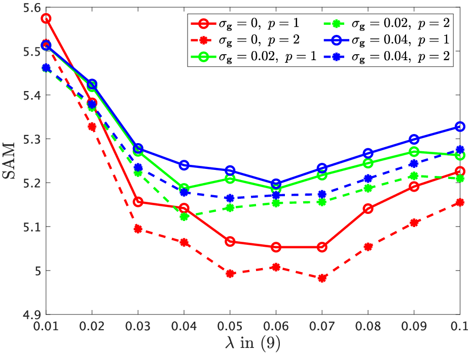
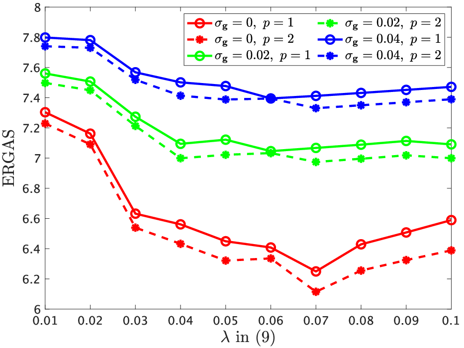
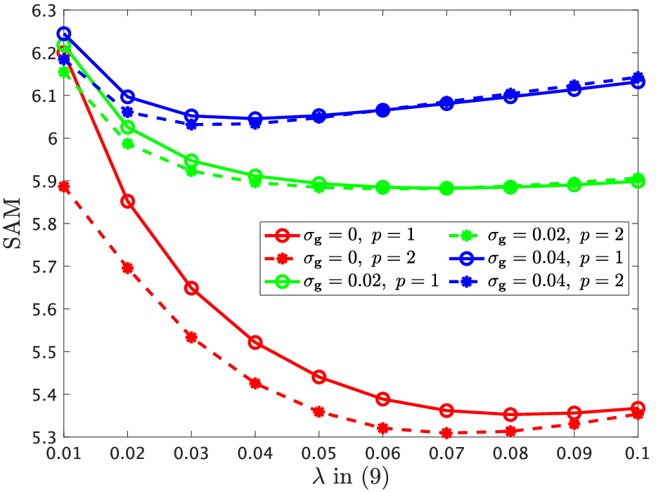
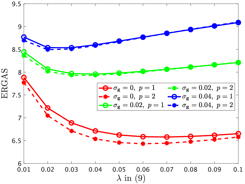
Fig 6 and 7 show $\omega$ and $\lambda$ versus four quality measures, respectively, where the graphs plot the average. In Fig. 6, one can see that the suitable $\omega$ is rarely affected by $r$ and $\sigma_{{\mathbf{g}}}$ . In PSNR, ERGAS, and $Q2^{n}$ , it is good that $\omega$ is set as less than 0.03, and For SAM, $\omega\in[0.070.1]$ is suitable. The two results are contrastive, so $\omega$ requires to be adjusted by what information one requires. In Fig. 7, one can see that the suitable $\lambda$ changes between SAM and the other quality measures. Since the hyperparameter $\lambda$ is the weight of the edge-similarity evaluation, the results are appropriate.

We plot the spatial and spectral response of the results in a Moffett field, $r=2$ , and $\sigma_{{\mathbf{g}}}=0.04$ case in Fig. 8. Here, we picked up the spatial vectors at the 43rd row and the 30th band of the results and the spectral vectors at the 43rd row and the 107th column of them. The graph of the spatial response shows that many methods produce artifacts, and the result by MTF-GLP has oversmoothing. Especially, the result by CNMF has some less than 0 value that cannot be actually observed value. GSA, GFPCA, and HySure suppress spatial artifacts compared with other existing methods, but the value of some pixels is significantly different, e.g., 13th, 53rd, and 120th elements. On the other hand, CNN-Fus and our proposed method can estimate spectral response without artifacts and oversmoothing compared with other methods. From the spectral response graph, one can see that CNMF suppresses intrinsic spectral response, and the results by GFPCA, CNMF, and CNN-FUS have spectral artifacts. In addition, one can also see that the values estimated by GSA, GFPCA, HySure, LTMR, and the proposed ( $p=2$ ) method are far apart with the large of the band number, and they are not good at estimating information of large wavelength. MTF-GLP, LTMR, and Lanaras’s produce the increase of spectral response that does not exist in the original in small bands. In contrast, the proposed ( $p=1$ ) method can estimate a more similar spectral response to the original one than the other methods. Based on the results of the spatial and spectral response, one can see that our method ( $p=1$ ) achieves effective spatial and spectral estimation.

We measured computational time, where we use Pavia U as a test HS image and set $r=2$ and $\sigma_{{\mathbf{g}}}=0.02$ . We conducted the experiments with MATLAB 2022a and a computer equipped with 64-GB random access memory and 12th Gen Intel(R) Core(TM) i9-12900K CPU with 3.2 GHz or NVIDIA GeForce RTX 3090. In Tab. VI, we align the computational time of all processing. In terms of the optimization-based methods and CNN-Fus, the table also shows the iteration number and endmember/abundance estimation time with the average time of each iteration. In this table, our methods spend much time compared with existing methods, but the iteration number is changed by image, noise intensity, degradation operator, and so on. From the time of each iteration, one can see that our methods achieve less computational time than existing optimization-based methods and CNN-Fus. Moreover, one can see that GSA, MTF-GLP, and GFPCA achieve less computational time than other methods, but they require a pre-denoising step, so one needs to consider the time of the step. In the pre-denoising process, FFDNet and FGSLR spend 0.1210s and 246.4s for denoising a guide image and an LR-HS image, respectively.

V-B HS and MS Image Fusion

To verify the performance of our proposed method for HS and MS image fusion, we did an experiment that estimates an HR-HS image from a pair of LR-HS and MS images. Here, we assumed a 4-bands MS image, and ${\mathbf{R}}\in{\mathbb{R}}^{4N\times NB}$ in (10) was the spectral response of the IKONOS satellite. In addition, we set the standard deviations of ${\mathbf{n}}_{{\mathbf{v}}}$ in (9) and ${\mathbf{n}}_{{\mathbf{g}}}$ in (10) as $\sigma_{{\mathbf{v}}}=0.2$ and $\sigma_{{\mathbf{g}}}=0$ , $0.05$ and $0.1$ , respectively, for $r=2$ and $4$ cases. In the experiments on large downsampling ratio $r=8$ and $16$ , we set $\sigma_{{\mathbf{v}}}=0.1$ and $\sigma_{{\mathbf{g}}}=0.05$ and use only Reno and Pavia U because of the spatial size of the test image. We set the stepsizes $\gamma_{1}$ and $\gamma_{2}$ to $0.01$ and $0.5$ , respectively, as satisfied with the convergence condition.

In Tab. VII and VIII, we show four quality measures of the results on $r=2$ and $r=4$ , respectively. When the noiseless guide image ( $\sigma_{{\mathbf{g}}}=0$ ), Lanaras’s achieves the highest performance of all methods. However, the performance of Lanaras’s significantly decrease as the noise intensity is large. Even though the method considers noisy observations, one can see that the result is sensitive to noise in a guide image. In some cases, the results of CNN-Fus are better than the other methods. As mentioned in Sec. V-A, CNN-Fus has a serious problem, so in a real situation, the achievement of the performance is very difficult. GSA, MTF-GLP, and HySure outperform our methods in some cases, but the performance is affected by image. From the average of the results, one can see that our methods achieve the highest performance and the stable estimation of all methods from a noisy guide image.

Tab. IX shows the quality measures of the results, and one can see that CNN-Fus achieves the best performance. However, from the discussion in the above experiments, the setting of the iteration number is very difficult but essential. Therefore, in fact, it is difficult that CNN-Fus realizes the performance. For Reno, SAM of GSA, MTF-GLP, and HySure is superior to that of our methods about 0.3 0.7, but our methods greatly outperform them about from 1 to 5 in Pavia U cases. In PSNR, ERGAS, and $Q2^{n}$ , the table shows that our methods achieve the second performance, i.e., one can see that our methods can estimate a desirable HR-HS image in the stable estimation.

From the results of quality measures, our methods can estimate a higher-performance HR-HS image on average, but SAM shows that some methods achieve the higher of almost the same performance as our methods for Reno and Salinas. To deeply analyze the reason, we depict the SAM map of the results by GSA, MTF-GLP, GFPCA, HySure, CNN-Fus, and the proposed methods (Salinas, $r=4$ , and $\sigma_{{\mathbf{g}}}=0.05$ ) in Fig. 9. One can see that GSA, MTF-GLP, GFPCA, and HySure suppress the error of spectral angle in the smooth area, but in the high-variation area, e.g., circle objects in the upper of the result, they produce a large gap of spectral angle. CNN-Fus achieves reduced spectral angle gaps compared with them in the small area, but still remains several gaps (red area in the SAM map). In contrast, the SAM map of our methods rarely has red areas, so our proposed method can estimate spectral information with a smaller gap of spectral angles than the other methods in the high-variation area like the results on HS pansharpening.

Fig. 10 plots MSE, band-wise normalized MSE, and the band-wise mean luminance in Salinas, $r=2$ , and $\sigma_{{\mathbf{g}}}=0.05$ cases to verify ERGAS of the results by GSA, MTF-GLP, GFPCA, HySure, CNN-Fus, and the proposed method in more detail. The graph of MSE shows that our proposed method almost improves the estimation performance from existing methods, especially the MSEs from 60th to 70th bands are significantly reduced. However, in over 90th bands, the proposed method is inferior to existing methods in many bands. From the band-wise mean luminance graph, since these bands have low luminance, one can see that the proposed method is weak in the estimation of the low luminance bands like the HS pansharpening experiments. For this reason, the band-wise normalized MSEs of some bands are significantly high, so the ERGAS of the result by the proposed method is larger than the results by the existing methods. The graph of the band-wise normalized MSE shows that the proposed method overcomes the existing methods in the many bands and has a high estimation ability.

We show two results in Fig. 11, where they are depicted by RGB images with $R=16$ th $G=32$ nd $B=64$ th bands. The upper two rows are the results in Moffett fileld, $r=2$ , and $\sigma_{{\mathbf{g}}}=0.1$ case, and the lower two are that in Pavia U, $r=4$ , and $\sigma_{{\mathbf{g}}}=0.05$ case. One can see that GSA, MTF-GLP, GFPCA, CNMF, Lanaras’s, and LTMR produce spatial and/or spectral artifacts, and the results by CNN-Fus are spatial oversmoothing or artifacts. One can also see that HySure can estimate spatial information, but the results by HySure have a few different colors, e.g. square architecture of Moffett field and orange architecture in the top center of Pavia U. Therefore, one can see that HySure produces a little distortion in the spectral direction. In contrast, our methods can estimate an HR-HS image without spatial and spectral artifacts compared with existing methods.

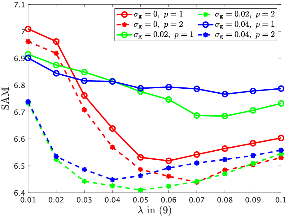
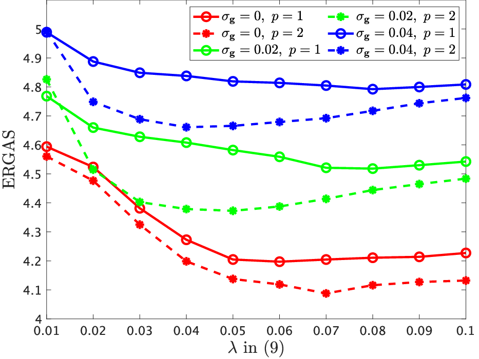
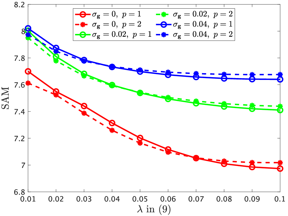
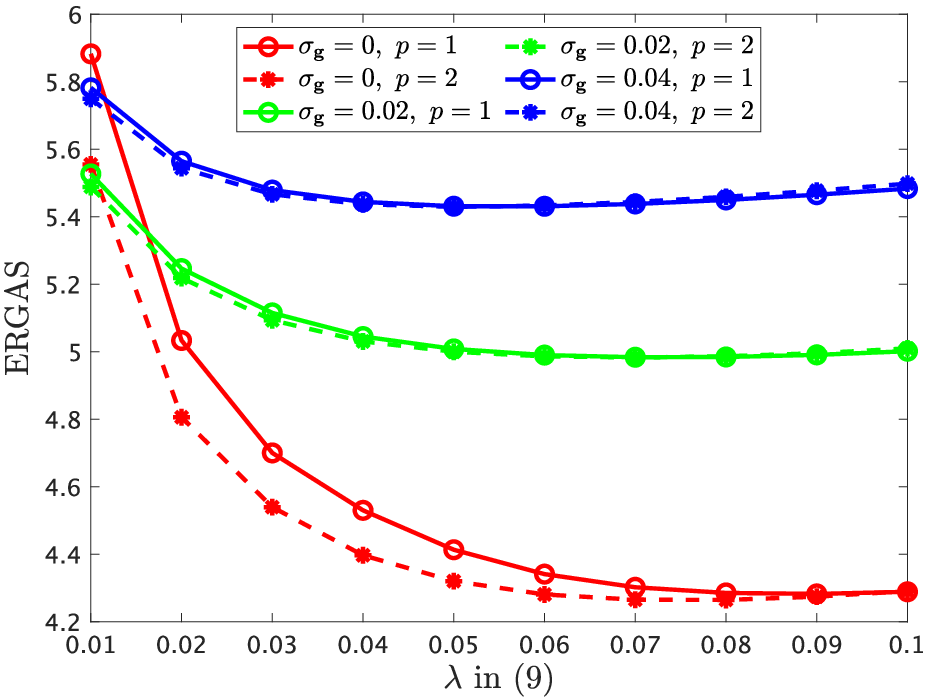
In Fig. 12 and 13, we plot $\omega$ and $\lambda$ versus four quality measures, where the top and bottom are the results in $r=2$ and $4$ cases, respectively. Fig. 12 shows that the suitable $\omega$ rarely changes by $r$ and $\sigma_{{\mathbf{g}}}$ in most cases. In PSNR, ERGAS, and $Q2^{n}$ , one can see that it is good that $\omega$ is set as less than 0.03. On the other hand, the graph shows that in SAM, the suitable $\omega$ value is from 0.03 to 0.05 different from the above quality measures. Fig. 13 shows that the suitable $\lambda$ is almost the same in different $\sigma_{{\mathbf{g}}}$ and $r$ cases, and $\lambda\in[0.07,~0.1]$ is good in most cases.

In Fig. 14, we plot the spatial and spectral response of the results in a Moffett field, $r=2$ , and $\sigma_{{\mathbf{g}}}=0.1$ case in like manner to HS pansharpening experiments. From the spatial response graph, one can see that other than GFPCA, HySure, and the proposed methods produce spatial artifacts. GFPCA, HySure, and our proposed method can reduce spatial artifacts and estimate some rapid spatial change. Especially, around the 40th elements and from the 45th to the 50th elements, the proposed methods can estimate a similar response to the original one than other methods. The spectral response graph shows that GFPCA, CNMF, HySure, Lanaras’s, and LTMR produce huge spectral artifacts. Moreover, one can see that the values estimated by GSA and MTF-GLP are far apart from the original after the 95th band. CNN-Fus can estimate similar spectral vectors to the original, but from the 10th to 40th bands, the spectral value significantly increases from the original. In contrast, our proposed methods can estimate more similar spectral responses to the original without spectral artifacts than other methods. From the above results, one can see that our method can estimate desirable spatial and spectral information.

VI Conclusion

We have proposed a new HR-HS estimation method based on convex optimization robust to noise in observations. Our method simultaneously estimates an HR-HS image and a noiseless guide image to suppress the effect of noise. The method can utilize the spatial detailed information in a guide image because it evaluates the edge-similarity between an HR-HS image and an estimated guide image. Moreover, it utilizes HSSTV to evaluate spatial and spectral piecewise smoothness of an HS image, which is TV-based regularization and achieves high performance for HS image denoising and compressed sensing reconstruction. Thanks to the design, the proposed method achieves robust HR-HS image estimation. To efficiently solve the problem, we adopt the primal-dual splitting method. In the experiments, we verify the performance of our method and illustrate the advantages over several existing methods.

Acknowledgment

This work was supported in part by JST PRESTO under Grant JPMJPR21C4, and in part by JSPS KAKENHI under Grant 22H03610, 22H00512, 21K21312, 20H02145, and 18H05413.

References

[1] C. I. Chang, Hyperspectral imaging: techniques for spectral detection and classification. Springer Science & Business Media, 2003, vol. 1.
[2] A. Plaza, J. A. Benediktsson, J. W. Boardman, J. Brazile, L. Bruzzone, G. Camps-Valls, J. Chanussot, M. Fauvel, P. Gamba, A. Gualtieri et al., “Recent advances in techniques for hyperspectral image processing,” Remote sensing of environment, vol. 113, pp. S110–S122, 2009.
[3] B. Rasti, P. Scheunders, P. Ghamisi, G. Licciardi, and J. Chanussot, “Noise reduction in hyperspectral imagery: Overview and application,” Remote Sens., vol. 10, no. 3, p. 482, 2018.
[4] L. Loncan, L. B. de Almeida, J. M. Bioucas-Dias, X. Briottet, J. Chanussot, N. Dobigeon, S. Fabre, W. Liao, G. A. Licciardi, M. Simoes et al., “Hyperspectral pansharpening: A review,” IEEE Geoscience and remote sensing magazine, vol. 3, no. 3, pp. 27–46, 2015.
[5] N. Yokoya, C. Grohnfeldt, and J. Chanussot, “Hyperspectral and multispectral data fusion: A comparative review of the recent literature,” IEEE Geoscience and Remote Sensing Magazine, vol. 5, no. 2, pp. 29–56, 2017.
[6] P. Chavez, S. C. Sides, J. A. Anderson et al., “Comparison of three different methods to merge multiresolution and multispectral data- landsat tm and spot panchromatic,” Photogrammetric Engineering and remote sensing, vol. 57, no. 3, pp. 295–303, 1991.
[7] C. A. Laben and B. V. Brower, “Process for enhancing the spatial resolution of multispectral imagery using pan-sharpening,” Jan. 4 2000, uS Patent 6,011,875.
[8] B. Aiazzi, S. Baronti, and M. Selva, “Improving component substitution pansharpening through multivariate regression of ms $+$ pan data,” IEEE Trans. Geosci. Remote Sens., vol. 45, no. 10, pp. 3230–3239, 2007.
[9] B. Aiazzi, L. Alparone, S. Baronti, A. Garzelli, and M. Selva, “Mtf-tailored multiscale fusion of high-resolution ms and pan imagery,” Photogrammetric Engineering & Remote Sensing, vol. 72, no. 5, pp. 591–596, 2006.
[10] G. Vivone, R. Restaino, M. D. Mura, G. Licciardi, and J. Chanussot, “Contrast and error-based fusion schemes for multispectral image pansharpening,” IEEE Geosci. and Remote Sens. Lett., vol. 11, no. 5, pp. 930–934, 2014.
[11] J. G. Liu, “Smoothing filter-based intensity modulation: A spectral preserve image fusion technique for improving spatial details,” International Journal of Remote Sensing, vol. 21, no. 18, pp. 3461–3472, 2000.
[12] W. Liao, X. Huang, F. V. Coillie, S. Gautama et al., “Processing of multiresolution thermal hyperspectral and digital color data: Outcome of the 2014 ieee grss data fusion contest,” IEEE Journal of Selected Topics in Applied Earth Observations and Remote Sensing, vol. 8, no. 6, pp. 2984–2996, 2015.
[13] M. Simões, J. Bioucas-Dias, L. B. Almeida, and J. Chanussot, “A convex formulation for hyperspectral image superresolution via subspace-based regularization,” IEEE Trans. Geosci. Remote Sens., vol. 53, no. 6, pp. 3373–3388, 2015.
[14] R. Dian and S. Li, “Hyperspectral image super-resolution via subspace-based low tensor multi-rank regularization,” IEEE Trans. Image Process., vol. 28, no. 10, pp. 5135–5146, 2019.
[15] Y. Yang, C. Wang, Y. Feng, J. Zhang, Y. Zheng, and S. Chen, “Regularizing subspace representation for fusing hyperspectral and multispectral images,” IEEE Selected Topics Appl. Earth Obser. Remote Sens., vol. 14, pp. 12 273–12 286, 2021.
[16] J. Ying, H. Shen, and S. Cao, “Unaligned hyperspectral image fusion via registration and interpolation modeling,” IEEE Trans. Geosci. Remote Sens., vol. 60, pp. 1–14, 2021.
[17] N. Yokoya, T. Yairi, and A. Iwasaki, “Coupled nonnegative matrix factorization unmixing for hyperspectral and multispectral data fusion,” IEEE Trans. Geosci. Remote Sens., vol. 50, no. 2, pp. 528–537, 2012.
[18] Q. Wei, J. Bioucas-Dias, N. Dobigeon, J. Tourneret, M. Chen, and S. Godsill, “Multiband image fusion based on spectral unmixing,” IEEE Trans. Geosci. Remote Sens., vol. 54, no. 12, pp. 7236–7249, 2016.
[19] C. Lanaras, E. Baltsavias, and K. Schindler, “Hyperspectral super-resolution by coupled spectral unmixing,” in Proc. IEEE Int. Conf. Comput. Vis. (ICCV), 2015, pp. 3586–3594.
[20] W. He, Y. Chen, N. Yokoya, C. Li, and Q. Zhao, “Hyperspectral super-resolution via coupled tensor ring factorization,” Pattern Recognition, vol. 122, p. 108280, 2022.
[21] P. Liu and L. Xiao, “A nonconvex pansharpening model with spatial and spectral gradient difference-induced nonconvex sparsity priors,” IEEE Trans. Geosci. Remote Sens., vol. 60, pp. 1–15, 2021.
[22] X. Tian, Y. Chen, C. Yang, and J. Ma, “Variational pansharpening by exploiting cartoon-texture similarities,” IEEE Trans. Geosci. Remote Sens., vol. 60, pp. 1–16, 2021.
[23] Y. Qu, H. Qi, C. Kwan, N. Yokoya, and J. Chanussot, “Unsupervised and unregistered hyperspectral image super-resolution with mutual dirichlet-net,” IEEE Trans. Geosci. Remote Sens., vol. 60, pp. 1–18, 2021.
[24] R. Dian, S. Li, A. Guo, and L. Fang, “Deep hyperspectral image sharpening,” IEEE Trans. Neural Networks and Learning Systems, vol. 29, no. 11, pp. 5345–5355, 2018.
[25] J. Yang, L. Xiao, Y. Zhao, and J. C. Chan, “Variational regularization network with attentive deep prior for hyperspectral–multispectral image fusion,” IEEE Trans. Geosci. Remote Sens., vol. 60, pp. 1–17, 2021.
[26] Z. Wu, T. Huang, L. Deng, G. Vivone, J. Miao, J. Hu, and X. Zhao, “A new variational approach based on proximal deep injection and gradient intensity similarity for spatio-spectral image fusion,” IEEE Selected Topics Appl. Earth Obser. Remote Sens., vol. 13, pp. 6277–6290, 2020.
[27] J. Qu, Y. Shi, W. Xie, Y. Li, X. Wu, and Q. Du, “Mssl: Hyperspectral and panchromatic images fusion via multiresolution spatial–spectral feature learning networks,” IEEE Trans. Geosci. Remote Sens., vol. 60, pp. 1–13, 2021.
[28] R. Dian, S. Li, and X. Kang, “Regularizing hyperspectral and multispectral image fusion by cnn denoiser,” IEEE Trans. Neural Netw. Learn. Syst., vol. 32, no. 3, pp. 1124–1135, 2020.
[29] S. Takeyama, S. Ono, and K. I, “A constrained convex optimization approach to hyperspectral image restoration with hybrid spatio-spectral regularization,” Remote Sensing, vol. 12, no. 21, p. 3541, 2020.
[30] N. Yokoya, T. Yairi, and A. Iwasaki, “Hyperspectral, multispectral, and panchromatic data fusion based on coupled non-negative matrix factorization,” in Workshop on Hyperspectral Image and Signal Processing: Evolution in Remote Sensing (WHISPERS), 2011, pp. 1–4.
[31] J. J. Moreau, “Fonctions convexes duales et points proximaux dans un espace hilbertien,” C. R. Acad. Sci. Paris Ser. A Math., vol. 255, pp. 2897–2899, 1962.
[32] H. H. Bauschke and P. L. Combettes, Convex analysis and monotone operator theory in Hilbert spaces. New York: Springer, 2011.
[33] A. Chambolle and T. Pock, “A first-order primal-dual algorithm for convex problems with applications to imaging,” J. Math. Imaging and Vision, vol. 40, no. 1, pp. 120–145, 2010.
[34] L. Wald, T. Ranchin, and M. Mangolini, “Fusion of satellite images of different spatial resolutions: Assessing the quality of resulting images,” Photogrammetric Engineering & Remote Sensing, vol. 63, no. 6, pp. 691–699, 1997.
[35] S. Takeyama, S. Ono, and I. Kumazawa, “Mixed noise removal for hyperspectral images using hybrid spatio-spectral total variati,” in Proc. IEEE Int. Conf. Image Process. (ICIP), 2019, pp. 3128–3132.
[36] S. Takeyama and S. Ono, “Joint mixed-noise removal and compressed sensing reconstruction of hyperspectral images via convex optimization,” in Proc. IEEE Int. Geosci. Remote Sens. Symp. (IGARSS), 2020, pp. 1492–1495.
[37] ——, “Compressed hyperspectral pansharpening,” in Proc. IEEE Int. Conf. Image Process. (ICIP), 2020, pp. 2855–2859.
[38] S. Takeyama, S. Ono, and I. Kumazawa, “Hyperspectral image restoration by hybrid spatio-spectral total variation,” Proc. IEEE Int. Conf. Acoust., Speech, Signal Process. (ICASSP), pp. 4586–4590, 2017.
[39] ——, “Hybrid spatio-spectral total variation: A regularization technique for hyperspectral image denoising and compressed sensing,” arXiv preprint arXiv:1907.13357, 2019.
[40] C. Chen, Y. Li, W. Liu, and J. Huang, “Image fusion with local spectral consistency and dynamic gradient sparsity,” in Proc. IEEE Conf. Comput. Vis. Pattern Recognit. (CVPR), 2014, pp. 2760–2765.
[41] M. V. Afonso, J. M. Bioucas-Dias, and M. A. Figueiredo, “An augmented lagrangian approach to the constrained optimization formulation of imaging inverse problems,” IEEE Trans. Image Process., vol. 20, no. 3, pp. 681–695, 2011.
[42] G. Chierchia, N. Pustelnik, J.-C. Pesquet, and B. Pesquet-Popescu, “Epigraphical projection and proximal tools for solving constrained convex optimization problems,” Signal, Image and Video Process., vol. 9, no. 8, pp. 1737–1749, 2015.
[43] S. Ono and I. Yamada, “Signal recovery with certain involved convex data-fidelity constraints,” IEEE Trans. Signal Process., vol. 63, no. 22, pp. 6149–6163, 2015.
[44] S. Ono, “Efficient constrained signal reconstruction by randomized epigraphical projection,” in Proc. IEEE Int. Conf. Acoust., Speech, Signal Process. (ICASSP), 2019, pp. 4993–4997.
[45] “SpecTIR,” http://www.spectir.com/free-data-samples/.
[46] “GIC,” http://www.ehu.eus/ccwintco/index.php?title=Hyperspectral_
Remote_Sensing_Scenes.
[47] Y. Chen, T. Z. Huang, W. He, X. L. Zhao, H. Zhang, and J. Zeng, “Hyperspectral image denoising using factor group sparsity-regularized nonconvex low-rank approximation,” IEEE Trans. Geosci. Remote Sens., vol. 60, pp. 1–16, 2021.
[48] K. Zhang, W. Zuo, and L. Zhang, “Ffdnet: Toward a fast and flexible solution for cnn-based image denoising,” IEEE Trans. Image Process., vol. 27, no. 9, pp. 4608–4622, 2018.
[49] F. Kruse, A. Lefkoff, J. Boardman, K. Heidebrecht, A. Shapiro, P. Barloon, and A. Goetz, “The spectral image processing system (SIPS)—interactive visualization and analysis of imaging spectrometer data,” Remote Sensing of Environment, vol. 44, no. 2, pp. 145–163, 1993.
[50] L. Wald, “Quality of high resolution synthesised images: Is there a simple criterion?” in Third conference” Fusion of Earth data: merging point measurements, raster maps and remotely sensed images”, 2000, pp. 99–103.
[51] A. Garzelli and F. Nencini, “Hypercomplex quality assessment of multi/hyperspectral images,” IEEE Geosci. and Remote Sens. Lett., vol. 6, no. 4, pp. 662–665, 2009.
[52] Z. Wang and A. C. Bovik, “A universal image quality index,” IEEE Signal Process. Lett., vol. 9, no. 3, pp. 81–84, 2002.

Saori Takeyama Saori Takeyama (S’17-M’21) received a B.E. degree in Computer Science in 2016 and M.E. and Ph.D. degrees in Information and Communications Engineering in 2018 and 2021 from the Tokyo Institute of Technology, respectively. From April 2018 to March 2021, she was a Research Fellow (DC1) of the Japan Society for the Promotion of Science (JSPS). She is currently an Assistant Professor in the Department of Information and Communications Engineering, School of Engineering, Tokyo Institute of Technology. Her research interests include signal processing, hyperspectral imaging and processing, and mathematical optimization. Dr. Takeyama received the Young Researchers’ Award from the IEICE in 2019, the Student Conference Paper Award from the IEEE SPS Japan Chapter in 2020, and the Telecomsystem Technology Student Award from the Telecommunications Advancement Foundation in 2021.

Shunsuke Ono Shunsuke Ono (S’11-M’15) received a B.E. degree in Computer Science in 2010 and M.E. and Ph.D. degrees in Communications and Computer Engineering in 2012 and 2014 from the Tokyo Institute of Technology, respectively. From April 2012 to September 2014, he was a Research Fellow (DC1) of the Japan Society for the Promotion of Science (JSPS). He is currently an Associate Professor in the Department of Computer Science, School of Computing, Tokyo Institute of Technology. From October 2016 to March 2020 and from October 2021 to present, he was/is a Researcher of Precursory Research for Embryonic Science and Technology (PRESTO), Japan Science and Technology Corporation (JST), Tokyo, Japan. His research interests include signal processing, image analysis, remote sensing, mathematical optimization, and data science. Dr. Ono received the Young Researchers’ Award and the Excellent Paper Award from the IEICE in 2013 and 2014, respectively, the Outstanding Student Journal Paper Award and the Young Author Best Paper Award from the IEEE SPS Japan Chapter in 2014 and 2020, respectively, the Funai Research Award from the Funai Foundation in 2017, the Ando Incentive Prize from the Foundation of Ando Laboratory in 2021, and the Young Scientists’ Award from MEXT in 2022. He has been an Associate Editor of IEEE TRANSACTIONS ON SIGNAL AND INFORMATION PROCESSING OVER NETWORKS since 2019.