Weighted hazard ratio estimation for delayed and diminishing treatment effect

Let $t_{1}$,$t_{2}$,…,$t_{r}$ be the ordered failure times across both treatment arms, $d_{1j}$ and $d_{2j}$ be the number of deaths at $t_{j}$ in treatment and control arm respectively with $d_{j}$= $d_{1j}$ +$d_{2j}$ and $n_{1j}$ and $n_{2j}$ be the number of individuals at risk before $t_{j}$ with $n_{j}$ = $n_{1j}$ + $n_{2j}$. Let $X_{1},X_{2},\dots,X_{r}$ denote the treatment assignment where $X_{j}$=1 if the j-th subject is assigned to treatment arm and $X_{j}$=0 if assigned to control arm. The log-rank test statistic is defined as,

$\displaystyle\begin{split}Z=\frac{\sum_{j=1}^{r}(d_{1j}-e_{1j})}{(\sum_{j=1}^{r}V_{L})^{1/2}}\end{split},$

where $e_{1j}$= $\frac{n_{1j}d_{j}}{n_{j}}$ is the expected number of failure at time $t_{(j)}$ under the null hypothesis of equal survival curves. $V_{L}$ is the variance of the observed number of failures, $V_{L}$ = $\sum_{j=1}^{r}\frac{n_{1j}n_{2j}d_{j}(n_{j}-d_{j})}{n_{j}^{2}(n_{j}-1)}$. Under the null hypothesis of equal survival functions in the two treatment groups, asymptotically the test statistic has a chi-squared distribution on one degree of freedom. Although the log rank test is still a valid test under non proportional hazards it is not the most powerful test [5]. Therefore, the weighted version of log rank test is sometimes utilised when the ratio of the two hazard functions are not constant over time [6].

The weighted log rank test (WLRT) assigns a weight function to different time points depending on the expected type of non-proportional hazard scenario. For instance, in immuno-oncology trials there may be a delayed treatment effect and therefore the survival curve for the treatment group will only emerge to separate from the control survival curve after a certain period of time. In this case, higher weights can be allocated to later time points [7]. Formally, the WLRT is defined as,

$$\begin{split}W_{K}=\frac{\sum_{j=1}^{r}w(t_{j})(d_{1j}-e_{1j})}{(\sum_{j=1}^{r}V_{L})^{1/2}}\end{split},$$

(1)

with variance

$\displaystyle\begin{split}V_{K}=\sum_{j=1}^{r}w(t(j))^{2}\bigg(\frac{n_{1j}n_{2j}d_{j}(n_{j}-d_{j})}{n_{j}^{2}(n_{j}-1)}\bigg)\end{split}$

where $w(\cdot)$ is the non-negative weight function. We will consider the Fleming-Harrington family of weighted log rank test, commonly denoted as $G^{\rho,\gamma}$ with weight,

$$w(t)=\hat{S}(t)^{\rho}(1-\hat{S}(t))$$

(2)

where $\hat{S}(t)$ is the Kaplan- Meier estimate of the survival function of the pooled patients from the treatment and control arm. The parameters $\rho$ and $\gamma$ control the shape of the weight function. $G^{0,0}$ represents the log-rank test with $w(t)=1$ that has constant weight over time; delayed treatment effects can be tested using $G^{0,\gamma}$ with $w(t)=(1-\hat{S}(t))$ that allocates higher weight at later time points to detect late survival difference, $G^{1,0}$ represents diminishing effect with $w(t)=\hat{S}(t)$ that gives more weight the earlier time points to detect early separation; $G^{1,1}$ represents mid separation with $w(t)=\hat{S}(t)(1-\hat{S}(t))$ that puts more weight at the middle of the follow-up period than at the ends.

Lin and León [8] proposed fitting a Cox model to provide a time varying treatment effect estimate to complement the weighted log rank test. Lin and León propose fitting a Cox model with,

$$\lambda(t;X)=\lambda_{0}(t)e^{A(t)\beta X}$$

where $A(t)$ is defined by,

$$A(t)=\frac{w(t)}{\textrm{max}(w(s))}$$

$\textrm{max}(w(s))$ is evaluated over the values of $t$ in the observed dataset and $A(t)$ thus has a maximum value of 1. The time varying covariate $X^{*}(t)=A(t)X$ represents the treatment assignment weighted by the adjustment factor. Once $X^{*}(t)$ has been determined, the constant coefficient $\beta$ can be estimated. It is shown in the paper that the score test of the null hypothesis that $\beta=0$ in the proposed model above is equivalent to the weighted log rank test with the corresponding choice of weight function [8]. Lin and León used the fact that the score test from this Cox model corresponds to a particular weighted log rank to motivate estimating the time-varying treatment effect using this Cox model. The coefficient $\beta$ can be interpreted as the maximal effect where the model assumes the patients experience the most benefit ($A(t)=1$). To differentiate the time varying hazard ratio derived from the proposed method, we will denote this as $HR_{LL}$ and it can be expressed as,

$$HR_{LL}(t)=\frac{\lambda_{0}(t)e^{A(t)\beta\times 1}}{\lambda_{0}(t)e^{A(t)\beta\times 0}}=e^{\beta A(t)}=\big[HR^{F}\big]^{A(t)}$$

(3)

where $HR^{F}$=$e^{\beta}$ represents the maximal effect (i.e., at time $t$ with $A(t)$=1). The time profile of the treatment effect can be observed as the treatment coefficient $\beta$ weighted by the adjustment factor $A(t)$. The estimate derived from the model provides a consistent time profile of the hazard ratio over time given that the true hazard ratio also varies over time as specified by $A(t)$. If this does not hold then the treatment effect measure will in general no longer be unbiased for the true value of the hazard ratio at a given time.

Fleming and Harrington [1] showed that the $G^{\rho}$ test statistic is the most powerful test statistic when the hazard ratio at time $t$ is of the following form,

$$\frac{\lambda_{2}(t)}{\lambda_{1}(t)}=\frac{e^{\Delta}}{\{S_{1}(t)\}^{\rho}+e^{\Delta}[1-\{S_{1}(t)\}^{\rho}]}$$

(4)

where $S_{1}(t)=\exp\left(-\int_{0}^{t}\lambda_{1}(x)\textrm{dx}\right)$ is the survival function for the control arm. The parameter $e^{\Delta}$ represents the hazard ratio at $t=0$. The parameter $\rho$ controls how quickly the effect diminishes. The above hazard ratio function (4) has its full treatment effect initially $e^{\beta}$ and decreases monotonically to 1. Later, we will demonstrate various examples with $\rho=0.5,1,2$ to further develop our understanding about the behaviour of the weighted logrank test and the proposed model. We now calculate the weighted hazard ratio function proposed by Lin and León [8] under the set up where the $G^{\rho}$ test statistic would be optimal. In order to calculate the proposed weighted hazard ratio function under the set up where WLRT is optimal, we will need to derive the true pooled survival function which is determined by finding the survival function of the two treatment arms. The hazard function for the treatment arm $\lambda_{2}(t)$ can be derived, assuming that the true data generating mechanism is such that that WLRT is optimal, by using equation (4)

$\displaystyle\begin{split}\lambda_{2}(t)&=\frac{\lambda_{1}(t)e^{\Delta}}{\{S_{1}(t)\}^{\rho}+e^{\Delta}[1-\{S_{1}(t)\}^{\rho}]}\\ \end{split}$

Thus, the survival function for the treatment arm is,

$$\begin{split}S_{2}(t)&=\exp\left(-\int_{0}^{t}\lambda_{2}(x)\textrm{dx}\right)\\ &=\exp\left(-\int_{0}^{t}\frac{\lambda_{1}(x)e^{\Delta}}{\{S_{1}(x)\}^{\rho}+e^{\Delta}[1-\{S_{1}(x)\}^{\rho}]}dx\right)\end{split}$$

(5)

We can replace the adjustment factor $A(t)$ with the weight function that the Lin and León method converges to (as $n$ tends to $\infty$) (3), in this case $S(t)$. For the Lin and León [8] method, we estimate the pooled survival function $S(t)^{\rho}$ by the Kaplan-Meier estimator for the pooled sample which is consistent for the true pooled survival function. Therefore the Lin and León method consistently estimates,

$$\begin{split}HR_{LL}(t)=e^{\beta A(t)}=e^{\beta\big(0.5S_{1}(t)+0.5S_{2}(t)\big)^{\rho}}\end{split}$$

(6)

Substituting $S_{2}(t)$ in the hazard ratio function (6) for which this WLRT is optimal for gives,

$$\begin{split}HR_{LL}(t)=\textrm{exp}\left[\beta\left(\frac{1}{2}S_{1}(t)\right)+\frac{1}{2}\exp\left(-\int_{0}^{t}\frac{\lambda_{1}(x)e^{\Delta}}{\{S_{1}(x)\}^{\rho}+e^{\Delta}[1-\{S_{1}(x)\}^{\rho}]}dx\right)\Bigg)^{\rho}\right]\end{split}$$

(7)

When fitting the proposed model, the $\beta$ is estimated from the Cox PH model once the adjustment factor $A(t)$ is determined. Comparing the true hazard ratio function (4) with the proposed hazard ratio function (7), we see that the two expressions do not appear to be equal to each other. In Appendix B, we demonstrate that the two hazard ratio functions are approximately equal to each other when $\Delta$ is close to 0. We also demonstrate this equality graphically in the next section where we choose the value of $e^{\Delta}$ to compare the hazard ratio functions. We also compare the hazard ratio expressions analytically for some particular choices of $\lambda_{1}(t)$ and $e^{\Delta}$ to illustrate in Appendix A.

The paper by Garès [9] has provided an expression for the hazard function for which the Fleming-Harrington test $G$ for detecting late effects is optimal. Assume, the survival time in the control arm is exponentially distributed with some constant hazard $\lambda_{1}$. Then Garès et al [9] show that the $G$ test is optimal for testing the hypothesis,

$$\begin{split}H_{0}:\lambda_{CT}&=\lambda_{TRT}=\lambda_{1}\\ H_{1}:\lambda_{TRT}(t)&=\lambda_{CT}\frac{L((\mathcal{L})^{-1}(\mathcal{L}(e^{-\lambda_{1}t})+\varphi))}{L(e^{-\lambda_{1}t})}\end{split}$$

(8)

where $L(x)=\int_{x}^{1}\frac{(1-s)}{s}ds=1+\ln(x)-x$ and $\mathcal{L}(x)=\int_{0.5}^{x}\frac{1}{s\log(s)+s-s^{2}}ds$. The expression for the hazard ratio has no closed form and needs numerical integration techniques to compute. Garès et al [9] has provided the definition for the parameter $\varphi$ which is evaluated at some chosen time point $\tau$ and is of the following form,

$$\begin{split}\varphi&=\mathcal{L}(r(1-S_{1}(\tau))+S_{1}(\tau))-\mathcal{L}(S_{1}(\tau))\\ &=\mathcal{L}(S_{2}(\tau))-\mathcal{L}(S_{1}(\tau))\end{split}$$

(9)

where $r$ is the discrepancy rate, $r=\frac{S_{2}(\tau)-S_{1}(\tau)}{1-S_{1}(\tau)}$.

Similar to the diminishing effect scenario, we can check whether the true hazard ratio for which the $G$ test is optimal, as given in equation (8), agrees with the hazard ratio estimation proposed by Lin and León [8]. The true hazard ratio under which the $G$ test statistic is optimal is shown to be the second equation in (8). Now the the weighted hazard ratio model proposed by Lin and León corresponds to,

$\displaystyle\begin{split}HR_{LL}(t)=e^{\beta A(t)}&=e^{\beta\frac{w(t)}{max(w(s))}}\\ &=e^{\beta\left(\frac{\left(1-S(t)\right)}{max(w(s))}\right)}=e^{\beta\left(\frac{(1-0.5S_{1}(t)-0.5S_{2}(t))}{max(w(s))}\right)}\end{split}$

From Garès et al, the survival in the treatment and control arm is defined as $S_{2}(t)=(\mathcal{L})^{-1}(\mathcal{L}(e^{-\lambda_{1}t})+\mathcal{L}(S_{2}(\tau))-\mathcal{L}(S_{1}(\tau)))=(\mathcal{L})^{-1}(\mathcal{L}(e^{-\lambda_{1}t})+\varphi)$ and $S_{1}(t)=e^{-\lambda_{1}}t$ [9]. We now substitute in for $S_{1}(t)$ and $S_{2}(t)$,

$$\begin{split}HR_{LL}(t)&=e^{\beta\left(\frac{\left(1-0.5e^{-\lambda_{1}t}-0.5\mathcal{L}^{-1}(\mathcal{L}(e^{-\lambda_{1}t})+\varphi)\right)}{\left(1-0.5e^{-\lambda_{1}\tau}-0.5\mathcal{L}^{-1}(\mathcal{L}(e^{-\lambda_{1}\tau})+\varphi)\right)}\right)}\end{split}$$

(10)

We assume that the Lin and León method estimates the correct hazard ratio ($e^{\beta}$) at the time point in the study where it is the biggest effect i.e. at $t=\tau$. Like in Section 3.1, we show that if the Lin and León method estimates the correct hazard ratio at the time point when it is largest, then it will estimate the HR at all other times correctly too. In Appendix C, we see that the expression for the hazard ratio function from Lin and León model (10) does approximately match the true HR assumed as per equation (8) under the condition that $\varphi$ is small.

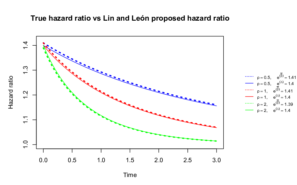
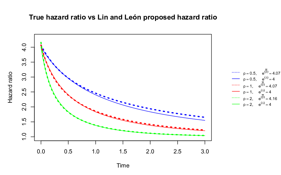
We simulated the survival data where the treatment is assumed to have its maximal effect initially and decrease monotonically to 1. The survival function for the treatment arm is given in equation (5). Three different scenarios $\rho=0.5,1,2$ were considered to understand the behaviour of the proposed model under various rates at which the effect diminishes. We also chose three different values of the maximum effect $e^{\Delta}=1.4,4,8$ to investigate whether substantial bias occurs when the treatment effect is larger. We fitted the Cox model proposed by [8] where the weight function $w(t)=\hat{S}(t)^{\rho}$ for the non PH data we simulated is specified for three scenarios $\rho=0.5,1,2$. The study enrolls 200 patients, equally allocated in the two arms. The survival of the control arm follows an exponential distribution with hazard rate $\lambda_{1}=0.5$. The survival in the treatment arm is as per equation (5) . The follow up time is assumed to be 3 years; patients whose event time exceeds 3 years are censored. We conduced 5000 runs for each scenario.

Figure 2 shows the true hazard ratio over time for which the $G^{\rho}$ statistic is optimal and the average hazard ratio profile over time estimated by the Lin and Leòn method. The plot displays $e^{\bar{\hat{\beta}}S(t)^{\rho}}$ where $\bar{\hat{\beta}}$ is the average of the hazard ratio at $t=0$ estimated from the Lin and Leòn method and $S(t)$ is the true pooled survival function. The proposed model overestimates the maximal effect when the true $HR$ at $t=0$ i.e. $e^{\Delta}$ is large, and slightly underestimates immediately after 1 month of follow up. Note that when the treatment effect is small, the proposed model estimates the maximal effect very close to the true one, in line with our analytical results in Appendix B. We observe through our work that when the treatment effect is large, the proposed model is not able to estimate the maximal effect at $t=0$ correctly which has an impact on the treatment effect profile over time, in that case the implied profile of treatment effect over time would not match the true one (as given by equation (4)).

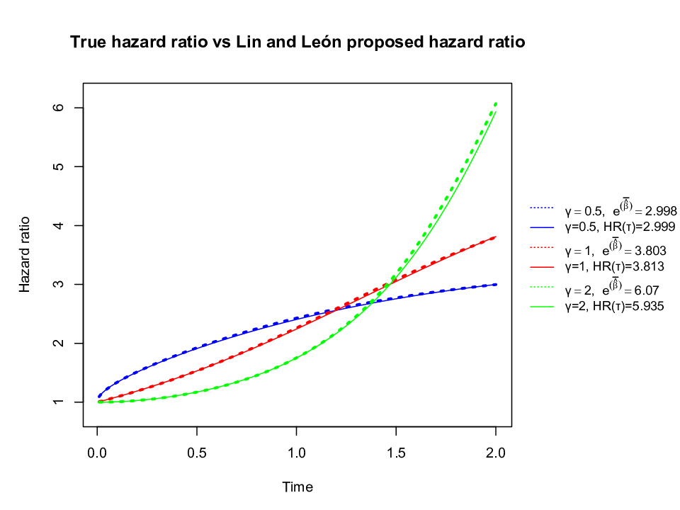
In this scenario, the data were simulated based on the assumption that the treatment will have no effect at the start of the follow up and gradually increases to have its maximal effect at the final time point of follow up period. The study enrolls the same number of patients as in the diminishing effect scenario i.e. 200. The maximal treatment effect occurs at the final time point $\tau=2$. The survival times in the control arm are exponentially distributed with hazard rate 0.5. The survival times in the active arm can then be simulated using the expression for the hazard function given in (8). To simulate the survival times in the active arm, we calculated the value of $S_{2}(t)$ for $t$ from 0 to $\tau$ in increments of 0.0005. We then simulated $U\sim U(0,1)$ and found the value of $t$ such that $S_{2}(t)$ was closest to $U$. We consider two scenarios of $S_{2}(\tau)=0.25$ and 0.1 which provides the values of discrepancy rate $r=-0.19$ and $-0.42$ for $\gamma=0.5,1,2$ to verify our results obtained in Section 3. The mechanism behind simulating the non proportional data in this way would ensure that the weight function $(1-S(t))$ would provide the most powerful test statistic. Similar to the previous scenario, we applied the Lin and León Cox PH model to our simulated datasets and compared the estimated HR profile with the true HR profile over time. We again considered three scenarios of $\gamma$ where it is varied to control the rate of how quickly the treatment effect reaches its maximum effect.

The true hazard ratio over time for which the $G$ statistic is optimal and the average hazard ratio profile over time estimated by the Lin and Leòn method is displayed in Figure 3. The plot displays the three HR profiles over time for $\gamma=0.5,1,2$ for two different values of $S_{2}(\tau)$. The solid lines represents the true HR profile and the dashed lines represents $e^{\bar{\hat{\beta}}(1-S(t)}$. Note that for both values of $S_{2}(\tau)$, the estimated average hazard ratio is overestimated for $\gamma=1,2$ and this deviation is reflected on the HR time profile. Though for other scenarios, we see that the Lin and León method estimates the treatment effect profile over time with minimal bias, in line with our analytical results in Appendix C.The proposed model closely estimates the maximal treatment effect for both scenarios where $\gamma=0.5$ and $r$ is relatively small.

References

- [1] Thomas R. Fleming and David P. Harrington. Counting processes and survival analysis, chapter 7, pages 255–277. A-Wiley-Intersciemce publication, 1991.
- [2] Tony S Mok, Yi-Long Wu, Sumitra Thongprasert, Chih-Hsin Yang, Da-Tong Chu, Nagahiro Saijo, Patrapim Sunpaweravong, Baohui Han, Benjamin Margono, Yukito Ichinose, et al. Gefitinib or carboplatin–paclitaxel in pulmonary adenocarcinoma. N England Journal of Medicine, 361(10):947–957, 2009.
- [3] G Kristensen, T Perren, W Qian, J Pfisterer, JA Ledermann, F Joly, MS Carey, PJ Beale, A Cervantes, AM Oza, et al. Result of interim analysis of overall survival in the gcig icon7 phase iii randomized trial of bevacizumab in women with newly diagnosed ovarian cancer. Journal of Clinical Oncology, 29(18_suppl):LBA5006–LBA5006, 2011.
- [4] Miguel A Hernán. The hazards of hazard ratios. Epidemiology (Cambridge, Mass.), 21(1):13, 2010.
- [5] Patrick Royston and Mahesh KB Parmar. Restricted mean survival time: an alternative to the hazard ratio for the design and analysis of randomized trials with a time-to-event outcome. BMC medical research methodology, 13(1):152, 2013.
- [6] Thomas R Fleming and David P Harrington. A class of hypothesis tests for one and two sample censored survival data. Communications in Statistics-Theory and Methods, 10(8):763–794, 1981.
- [7] Ray S Lin, Ji Lin, Satrajit Roychoudhury, Keaven M Anderson, Tianle Hu, Bo Huang, Larry F Leon, Jason JZ Liao, Rong Liu, Xiaodong Luo, et al. Alternative analysis methods for time to event endpoints under nonproportional hazards: A comparative analysis. Statistics in Biopharmaceutical Research, 12(2):187–198, 2020.
- [8] Ray S Lin and Larry F León. Estimation of treatment effects in weighted log-rank tests. Contemporary clinical trials communications, 8:147–155, 2017.
- [9] Valérie Garès, Sandrine Andrieu, Jean-François Dupuy, and Nicolas Savy. On the fleming—harrington test for late effects in prevention randomized controlled trials. Journal of Statistical Theory and Practice, 11(3):418–435, 2017.