Differentiable physics-enabled closure modeling for Burgers’ turbulencePreprint: AIP/123-QED
Abstract
Data-driven turbulence modeling is experiencing a surge in interest following algorithmic and hardware developments in the data sciences. We discuss an approach using the differentiable physics paradigm that combines known physics with machine learning to develop closure models for Burgers’ turbulence. We consider the 1D Burgers system as a prototypical test problem for modeling the unresolved terms in advection-dominated turbulence problems. We train a series of models that incorporate varying degrees of physical assumptions on an a posteriori loss function to test the efficacy of models across a range of system parameters, including viscosity, time, and grid resolution. We find that constraining models with inductive biases in the form of partial differential equations that contain known physics or existing closure approaches produces highly data-efficient, accurate, and generalizable models, outperforming state-of-the-art baselines. Addition of structure in the form of physics information also brings a level of interpretability to the models, potentially offering a stepping stone to the future of closure modeling.
Keywords:
turbulence, burgers, subgrid-stress modeling, differentiable physics, machine learning, neural operatorsI Introduction
Simulation of fluid flow for practical applications is characterised by high Reynolds number turbulent flows over complex geometriesDeville, Fischer, and Mund 2002; Karniadakis 1999. The temporal and spatial scales of motion in such flows span several orders of magnitudeMoin and Mahesh 1998. The cost of Direct Numerical Simulations (DNS), which attempt to capture all energy containing lengthscales in the flow, grows superlinearly with the Reynolds number of the flowKolmogorov 1941; Coleman and Sandberg 2010; Orszag 1970, limiting the scope of fully resolving simulations to canonical geometries at medium Reynolds numbersMoin and Mahesh 1998.
Turbulence closure models have been developed for cases where resolving and evolving the entirety of velocity and pressure spectra is not possible. Techniques such as Large Eddy Simulations (LES) and Reynolds Averaged Navier-Stokes (RANS) allow for cheaper calculations of high Reynolds number flows by resolving only a portion of the spectrum and ‘modeling’ the rest Pope 2000. Put simply, the goal of turbulence modeling is to find a closed system that can describe the time-evolution of observables, such as the resolved velocity spectrum, via a ‘closure’ map that allows one to untangle the dependence of said observables on unresolved variablesSagaut 2006; Adams 2007; Qi and Harlim 2022.
The problem of turbulence closure modeling has been extensively studied for over a century, dating back to Boussinesq’s eddy viscosity hypothesis in 1877Layton 2014. More recently, machine learning (ML) based methods have utilized for modeling fluid flow problemsBrunton, Noack, and Koumoutsakos 2020; Vinuesa and Brunton 2021; Duraisamy, Iaccarino, and Xiao 2019; Kochkov et al. 2021; Watt-Meyer et al.; Vlachas et al. 2018; Thuerey et al. 2020; Portwood et al. 2021; Wang et al. 2020. The success of machine learning is built upon the ability of deep neural networks to approximate functions in high-dimensional spaces with a number of parameters that does not scale exponentially with the dimension of the problem spaceWeinan 2020. As the underlying problem in closure modeling is of finding the functional mapping between high-dimensional vector spaces, deep neural networks can be utilized in a supervised learning framework.
However, the performance of machine learning models to turbulence modeling has largely been unsatisfactory. A probable reason is that while neural networks are touted to break the curse of dimensionality, the cost of attaining an accurate model may be larger. The cost of generating high-fidelity data for the model does scale with dimensionalityPope 2000, and even if data is readily available, machine learning models need to be trained on large number of samples to accurately approximate even simple functions. In other words, an optimal closure model may be present in the space of functions that a neural network architecture can express, but there is no clear path towards realizing it.
Some success has been seen, however, by augmenting neural network models with physical priors. For example, Ling et al.Ling, Kurzawski, and Templeton 2016; Milani, Ling, and Eaton 2021 improved upon conventional machine learning models by embedding Galilean invariance in the prediction of Reynolds stress tensor for Reynolds Averaged Navier-Stokes simulations. Shankar et al. Shankar et al. 2020 enhanced the output of a convolutional neural network model on homogeneous isotropic turbulence by imposing the divergence-free constraint on the model output. Both approaches can be understood as attempts to narrow down the space of functions that a neural network architecture can represent.
Rackauckas et al.Rackauckas et al. 2020 further develops inductive biases in data-driven learning by directly embedding trainable parameters in a model’s governing differential equations. Training such parameters against a loss function that depends on the solution to the governing system requires passing gradient information through a differential equation solve. Therefore a solver that is compatible with automatic-differentiation toolchains in needed. Directly backpropagating gradients is computationally expensive for large solves, so the adjoint optimization methodChen et al. 2018; Farrell et al. 2013; Errico 1997; Sigmund and Maute 2013 is utilized. CFD codes such as SU2 have utilized the adjoint method for sensitivity analysis and shape optimizationPalacios et al. 2013.
This idea is formalized into the notion of Differentiable PhysicsRamsundar, Krishnamurthy, and Viswanathan 2021, defined as the set of scientific avenues emerging from the marriage of state-of-the-art partial differential equation (PDE) solvers with differentiable programming. The promise of differentiable physics is that machine learning models can be developed to learn specific unknown or residual physics, leading to more interpretable models than classical ML approaches. We envision the landscape of data-driven models on an axis of increasing inductive biases in Figure 1.
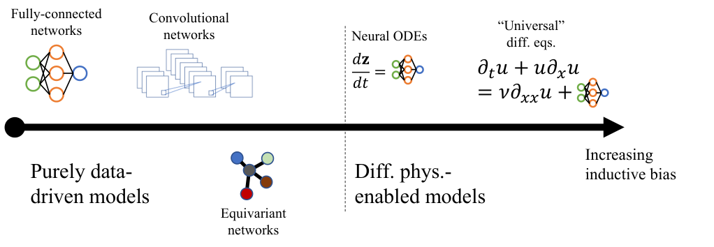
In this work, we comprehensively test the ability of ML techniques to develop turbulence closure models that are resolution independent, interpretable in the language of flow physics, and generalizeable across a range of Reynolds numbers. We consider the 1D Burgers system as the ideal test problem for modeling the energy spectra observed in advection-dominated turbulence problems, and narrow our focus to the task of subgrid-stress modeling. We test a range of differentiable physics models, that vary from a black-box approach to training coefficients in state-of-the-art turbulence models. Experiments are conducted over a range of Reynolds numbers and grid resolutions to assess the generalizability of the model, and over multiple resolution-independent architectures. We find that physics-based inductive biases are critical to the development of data-efficient and accurate ML closures, and that these ML closures can outperform state-of-the-art closure baselines in a wide range of flows.
II Background
II.1 Burgers Turbulence
Turbulent flows are characterised by a competition between viscous forces, which damp out velocity fluctuations by converting kinetic energy into heat, and inertial forces, such as gravitation or pressure gradients. These tend to generate and preserve velocity and pressure fluctuationsAlexander Smits 2013. In low Reynolds number flows, viscous forces dominate and the flow is near perfectly damped, meaning that any arbitrary fluctuation in the velocity field would be smoothed out in no timeThomas 1953. The velocity fields adjusts almost instantaneously to any changes in the pressure gradient that drives the flow. At high Reynolds numbers, however, viscous forces may not be strong enough to dampen out velocity fluctuations, and even tiny disturbances may cause the entire flow to destabilise into turbulenceRoberts 2020. Energy dissipation primarily happens at the smaller scales as the rate of dissipation scales with the wavenumber squared.
We restrict the scope of this work to the task of subgrid stress modeling in advection-dominated turbulence problems. The unforced, viscous Burgers problem, Eq. 1, an advection-diffusion type problemFrisch and Bec 2000 that exhibits an energy cascade similar to the Navier-Stokes system, is the perfect test bench. The Burgers system is governed by
| (1) |
where , the solution to the Burgers system, represents a time-varying velocity field and is the kinematic viscosity. The 1D viscous Burgers system is a canonical PDE that is widely used as a simplified case study for subgrid model development and analysis Falkovich and Sreenivasan 2006; Frisch and Bec 2000; Love 1980; LaBryer, Attar, and Vedula 2015. The nonlinear advective term coupled with viscous dissipation leads to similar multiscale phenomena observed in more complex flow dynamics. Eq. 1 is deterministic which allows us to directly compare trajectories rather than statistical averages, speeding up model training. We insulate the problem from arbitrary effects of boundary conditions by considering Eq. 1 on the entire real line, , which is approximated by periodic boundary conditions on an interval. The Burgers equation can also be written in its conservative form
| (2) |
which is typically more amenable to numerical calculation.
II.2 Large Eddy Simulations
As high Reynolds number flows have a wide energy spectrum, DNS of such flows is often computationally intractable, and a turbulence model is needed. Large Eddy Simulations (LES) resolves the flow variables starting from the intertial range up to a cut-off length, , that depends upon the computation gridLesieur and Metais 1996; Boris et al. 1992. Critically, an LES calculation ignores the smallest lengthscales in the flow, which are most computationally expensive to resolve. Filtering is accomplished by
| (3) | ||||
where is a low-pass filtering operator. Quantities of interest are interpolated onto a computational grid that can resolve flow features only up to lengthscale . The grid has much lower resolution than what is needed to fully resolve the flow, and evolving flow variables on this grid lead to saving computational resources.
Filtering the Burgers equation in this manner leads to
| (4) |
the LES equations for the Burgers system. Evolving per Eq. 4 is not possible as one does not have access to the subgrid stress term, , and ignoring it leads to an incorrect flow field and numerical instabilities. For the Navier-Stokes equations, ignoring subgrid stresses leads to numerical instabilities spurious high-frequency modesMullen and Fischer 1999. The closure problem of LES is of modeling the effect of on the dynamics of . This is called subgrid stress modeling. As one does not have access to the unresolved quantities, subgrid stress models are formulated in terms of the resolved quantities.
Kolmogorov hypothesized that the finer scales are largely similarKolmogorov 1941, and are primarily responsible for energy dissipation. One approach to closure modeling is to take out small amounts of energy from the high-frequency modes in by applying a mild low-pass filter at every timestep. Fisher et al.Mullen and Fischer 1999 has applied this methodology to the Navier-Stokes equations in the Computational Fluid Dynamics (CFD) code NEK5000Paul F. Fischer and Kerkemeier 2008, and Layton et al.Layton, Pruett, and Rebholz 2010 has prove existence of unique strong solutions to the resulting continuum model for the same.
Another approach is to directly model the commutative error term, in terms of with a map , and evolve the flow variables as per Eq. 4. Hypothesizing a functional form for additive closures of this sort is highly problem dependent. A common hypothesis is the eddy viscosity family of modelsFrisch and Kolmogorov 1995; Schmitt 2007 that introduce an “effective” or “eddy” viscosity, , to the momentum equation for enhancing dissipation. This leads to a functional form of , where could be a fixed scalar based on known flow physics and computational grid, or be defined by a transport equation. In § IV we consider several such models and apply them to the Burgers problem.
III Method
III.1 Numerical methods
We compute solutions to the Burgers equation via a pseudospectral method Boyd, Marilyn, and Eliot 2000. The periodic 1D domain is discretized with a regular grid of grid points. The periodic nature of the solutions allow for expansion in a Fourier basis, as per
| (5) |
The linear term of the equation can be computed pointwise in Fourier space
| (6) |
however the nonlinear term introduces interactions between all the wavemodes and thus requires more care for efficient computation. Therefore, it is more suitable to compute the quadratic term pointwise in real space at the collocation points, then compute the spatial derivative in Fourier space.
The spatial discretization allows for a method of lines approach to time evolution. The discrete Fourier modes from the spectral basis expansion produces a system of ordinary differential equations (ODEs) that can be solved with standard ODE integration schemes. We choose the Tsitouras adaptive 5th order scheme Tsitouras 2011.
III.2 Problem statement
Accurate simulation of the governing Burgers equation imposes certain restrictions on the temporal and spatial discretization. As we use an adaptive time-stepping scheme with fixed error tolerance, we focus on errors arising from the spatial discretization. The spatial grid should be sufficiently dense to resolve the smallest dissaptive length scales in the flow, typically much smaller than the characteristic length scales of the flow.
We wish to approximate solutions to the Burgers equation on a considerably coarser grid of points, by exploring a family of data-driven models enabled by algorithmic differentiation of the temporal and spatial discretization schemes. Each of the models is described by a PDE or set of PDEs, where certain terms in the equations are computed by deep neural networks. Thus, we enable significant interpretability of the models as network outputs can be readily identified as components of traditional closure modeling approaches.
III.3 Models
In this section, we provide a description of the various models that we use in our experiments. First, we make clear our notational conventions.
is the spatiotemporal velocity field we are modeling. is the filtered velocity field on the LES grid. We drop the parentheses for brevity. represents an unknown closure variable we are modeling. The exact description of this variable differs across models. In some models, an additional transport equation is introduced to govern the dynamics of the closure variable. The and the symbols correspond to the time derivative and spatial derivative of the field respectively. A subscript 0 represents the initial condition of the field.
Neural networks are indicated with subscript . These functions are parameterized by a large number of weights with functional form described in the subsequent section. Network inputs and outputs are written as:
| (7) |
where and are explicit inputs to the network, and and are outputs of the network with implicit dependence on variable . For example, represents a network that takes the spatially varying velocity field as input and produces a spatially varying field as output.
The ground truth equation, or none model, is given by:
| (8) |
Since there is no closure term or trainable networks, we use this as a baseline comparison for our learned models.
We also compare our models to a couple baseline closure models Maulik and San 2018, the constant Smagorinsky model (further denoted as smag-const), and the dynamic Smagorinsky model (further denoted as smag-dyn). The constant Smagorinsky modelSmagorinsky 1963 is given by:
| (9) |
| (10) |
where is the eddy viscosity, is the Smagorinsky constant, and is the grid spacing. While there are no trainable networks in this model, can be optimized via hand tuning or gradient descent.
The dynamic Smagorinsky model Germano et al. 1991; Lilly 1992 is similar to the constant model, however the term is determined from the state of the system. Studies have shown that is not constant and may be variable with different flow characteristics Smagorinsky 1993. The model uses a second test filter, denoted by with filter scale . We fix the filter ratio . Specifically,
| (11) |
| (12) |
| (13) |
where denotes averaging over the spatial domain.
The rest of the models in this section contain trainable networks in functional forms that rely on varying degrees of assumptions typically used in closure analysis. At one extreme, we have model resnet, which uses the classical ResNet architecture He et al. 2015 to predict the coarse-grained flow field at the next time step:
| (14) |
| (15) |
where is a coarse time step. This model makes no assumptions about the physical description of the system, including the fact that it may be described as a PDE. The closure variable is used only to lift the model into a higher-dimensional space governed by the neural network. The network may choose to learn , or it may leverage in the computation of . Projecting or transforming an input into a higher-dimensional subspace is a common practice in ML, where a large latent space of hidden channels eases learning. This is a core component of augmented neural ODEs Dupont, Doucet, and Teh 2019, which have shown to generalize better than standard neural ODEs.
anode, an augmented neural ODE, is a small modification to resnet that assumes an ODE inductive bias. The model is given by:
| (16) |
| (17) |
where explicitly describes the RHS of an ODE governing the discretized flow field. The dynamics of and are determined purely by the network with no additional terms. This involves only a small change in the code of resnet, changing the solver from explicit Euler to an adaptive scheme.
Filtering the governing equations as in Eq. 4 introduces an additional closure term to the equations. Model direct models the entirety of this term directly as an additive correction:
| (18) |
| (19) |
Model transport-I leverages the fact that the closure term can be written as the divergence of an unknown subgrid stress. Here, represents this stress analogue in 1D, which is additionally transported with another dynamical equation:
| (20) |
| (21) |
| (22) |
| (23) |
The coefficients of the dissipative and convective terms in the transport equation are given by neural networks.
Model transport-II uses the Boussinesq hypothesis that the subgrid stress has a linear relationship with the strain in the flow. represents an eddy viscosity analogue:
| (24) |
| (25) |
| (26) |
| (27) |
Model transport-I-p is nearly identical to transport-I, however the transport equation has an additional production term :
| (28) |
| (29) |
| (30) |
| (31) |
Model transport-II-p is equivalent to transport-II except for the additional production term:
| (32) |
| (33) |
| (34) |
| (35) |
The last model, smag-ml, attempts to improve on the standard constant Smagorinsky model by learning a spatially varying Smagorinsky constant, computed via neural network:
| (36) |
| (37) |
| (38) |
All of the models used in our analysis are tabulated in Table 5 of the appendix.
III.4 Neural network architecture
To leverage our choice of pseudospectral discretization, we use Fourier Neural Operators (FNO) as our network architecture Li et al. 2020. All functions with subscript in the previous section correspond to an FNO architecture. FNOs combine pointwise in real space and pointwise in Fourier space linear operations with pointwise nonlinearities in real space to enable learning of a large suite of resolution-invariant function classes, including linear and nonlinear operators.
Given an input feature , where is the number of channels or scalar fields, an FNO layer is defined as:
| (39) |
where is a 2-dimensional tensor that is contracted along identically pointwise in real space and is a 3-dimensional tensor that is contracted along pointwise in Fourier space for each wavemode up to . Therefore, the Fourier transform of the input is truncated at . The output of these operations are summed and a pointwise nonlinearity is applied. The parameters of the layer are given by the tensors and . Figure 2 illustrates the algorithm for in the smag-ml model.
III.5 Optimization
Network parameters are optimized with respect to the loss function:
| (40) |
| (41) |
where is the ground truth velocity field resolved on a grid of points, is filtered using sharp low-pass filter with cutoff , correspond to the collocation points on the coarse grid, and correspond to the timesteps in the discretized solution trajectory.
Optimization is achieved with the gradient-based optimizer ADAM, shown to be effective for deep learning applications Kingma and Ba 2015. Gradients are computed with the automatic differentiation (AD) platform available in Pytorch via reverse-mode autodifferentiation, or backpropagation Paszke et al. 2019. We show a schematic of the training procedure in Figure 3.
Most of the operations in our solution algorithm consist of basic linear operations and pointwise nonlinearities, operations that have formed the foundation of classical multi-layer perceptron machine learning architectures. Deep learning libraries have readily supported backpropagation through these operations for many years and thus we do not discuss implementation details further. However, we highlight two slightly more complex components of the algorithm corresponding to aspects of the spatial and temporal discretization and discuss their gradient computation.
III.5.1 Gradients of the Fourier transform
In reverse-mode gradient accumulation Speelpenning 1980, we wish to compute vector-Jacobian products (VJPs) Paszke et al. 2017; Griewank and Walther 2008 of each function in the algorithm:
| (42) |
given the cotangent vector , input , and Jacobian . The VJP can then be passed to the previous function in the computational graph to compute the next VJP.
We leverage spectral basis expansion to compute spatial derivatives in the flow and inside the FNO layers. This is implemented with a Discrete Fourier Transform (DFT) operation. Since the DFT is ultimately a linear operation
| (43) |
with DFT matrix , the Jacobian of the transform is simply the matrix . To compute the VJP, we can equivalently perform matrix-vector multiplication with the adjoint operator . Since , we can compute the VJP as an inverse Fourier transform multiplied by the size of the signal. The benefit of this approach comes from the ability to implement Fast Fourier Transform Frigo and Johnson 2005 (FFT) algorithms during the backwards pass as well, instead of constructing the entire DFT matrix explicitly.
III.5.2 Propagating gradients through time integration
Time evolution of the velocity field is accomplished by solving the ODE resulting from spatial discretization of the field using an arbitrary integration method. A naive implementation of AD would propagate gradients through each of basic operations in the solver. Depending on the solver tolerance, order, and trajectory length, this may result in a very large number of operations, and all intermediate steps must be saved in memory for AD to work. In our experiments, backpropagating through even moderately sized trajectory lengths, networks, and batch sizes could exceed the 16GBs of memory on our NVIDIA V100 GPU using naive autograd.
Therefore, a more memory efficient approach is desired. We use the adjoint method in time, which has been proposed for use in machine learning applications by Chen et. al Chen et al. 2018. The forward ODE system is given by the evolution of the discrete Fourier modes:
| (44) |
where represents any learnable parameters in the model. The loss can be written as an integral:
| (45) |
The adjoint method produces a second ODE system that evolves the adjoint variable backwards in time, given by the equation:
| (46) |
and an integral:
| (47) |
to compute the parameter sensitivities. The RHS of the equations involve VJPs that are efficiently evaluated with AD. The adjoint system can again be solved with an arbitrary solver, potentially even different than the forward solver. Specifically, we use the interpolated adjoint method, which reduces the memory footprint by constructing an interpolation of the forward solution, which appears in the adjoint equations. During the forward pass, the solution is saved at a selected few timesteps and reused in the adjoint computation via interpolation during the backwards pass.
IV Experiments and results
To assess the quality and practicality of our proposed models, we seek to study model performance across a range of Burgers solutions.
IV.1 Viscosity generalization and temporal stability
In this experiment, we examine model generalizability with respect to initial conditions of the velocity field and the viscosity parameter . In addition, we investigate stability of the models by extrapolating in time relative to the training data.
The models are trained using the optimization procedure described in the previous section on a ground truth dataset of 100 Burgers solutions. We vary the initial conditions of the velocity field by randomizing the Fourier modes of the initial field. The th Fourier mode is denoted by . The dataset is generated with the parameters tabulated in Table 1.
| Parameter | Range | ||
| , | |||
| 4096 | |||
| 64 |
The neural networks in the trainable models contain 2 FNO layers with , 128 hidden channels, and appropriate input and output sizes. The first layer uses a ReLU nonlinearity while the second uses the identity. The models are trained for 500 epochs using the ADAM optimizer with learning rate varying from to depending on the model. Generally, models such as smag-ml that are more constrained by inductive biases required larger learning rates.
Model performance is gauged using the mean-squared error of the predictions relative to the ground truth solution on an unseen test set. We leverage two test sets to assess generalizability across viscosities and stability in time. The first test set consists of solutions – 25 discrete viscosities in the range of – and 25 trajectories, or different initial conditions, per viscosity. We compute the model error for each prediction and plot the average ensemble error as a function of viscosity.
The second test set contains 25 trajectories at . Here, we evolve the trajectories between , over 3 times longer than the training set, to see how the models behave outside of the training regime. The average error across all trajectories is plotted as a function of time.
Two non-trainable models none and smag-const provide some bounding benchmarks for model comparison. In Figure 4(a), at the upper end, the none model with no closure results in high error at low viscosities, where the dissipative length scales are small, with progressively lower error at higher viscosities where the dissipative length scales become larger. An effective closure model should at the very least perform better than this, otherwise no additional physics have been learned to improve over the baseline governing equations solved on a coarse grid. At the lower end, the smag-const model is a well-known closure model that has been shown to perform well in a wide range of viscosities. An ideal model would produce lower loss than this baseline, indicating that the neural closure functional form can show improvements over classical closure models from theory.
Model performance is delineated well by model accuracy relative to the baselines in Figure 4(a). Model anode has the highest loss, greater than the none baseline, thus showing no improvement over the governing equations. Given that the anode model contains no inherent physics or structural form to the PDE, this result is unsurprising as the model must learn both the governing dynamics and any closure approximations. Despite resnet having a similar architecture to anode, resnet can achieve marginally better accuracy, although it is still no better than the none baseline. Theoretically, anode should be able to learn the same optima as resnet, since anode has the same functional form as resnet, except solved using an adaptive time-stepper. However, actually reaching those optima can be challenging during optimization due to the ODE inductive bias.
Models transport-I and transport-I-p show marginal improvement over none, with transport-I-p the better of the two. These models were particularly difficult to train, producing very stiff ODEs that made integration difficult. This is apparent in the fact that some of the viscosities are not shown as the stiffness of those systems led to intractable solutions. We hypothesize that this could be due to overfitting the training set, since all of the training samples could be solved in a reasonable amount of time.
Model direct lies firmly between the two benchmarks. Accuracy is relatively uniform with little dependency on viscosity. Thus, while direct consistently improves over none at low viscosities, the advantage decreases with increasing viscosity, becoming a disadvantage at the highest viscosities.
Models transport-II and transport-II-p have accuracies comparable to smag-const and perform almost identically to each other within the viscosity test. Generally, we see a consistent positive bias over the baseline closure benchmark that diminishes only at the highest viscosities.
Model smag-ml is the only model with lower error than smag-const everywhere in Figure 4(a). Given that the model leverages the functional form of the classical Smagorinsky model and only adds a spatial dependency, again this result is perhaps unsurprising. However, it is promising that the improvements persist beyond the training region.
Overall, besides models none, transport-I, and transport-I-p, accuracy is mostly independent of the viscosity within this range. While models have been trained on viscosities between and , they can be used on viscosities well outside this range, with little to no erroneous behavior outside the training regime.
Figure 4(b) shows model accuracy on the second test set. The blue region indicates the time span the model was trained on, while the red region shows the extrapolation range. The model hierarchy by accuracy is generally preserved here, i.e. anode performs the worst, smag-ml the best, and transport-II and transport-II-p are comparable to smag-const.
However, the stability test highlights the effect of the production term in the models. The models largely have a monotonically decreasing slope in the error over time, except for anode, transport-I-p, and transport-II-p, which display aberrant behavior in the extrapolation range. The inclusion of the production term results in improvements within the training time regime, and in the case of transport-I and transport-I-p, the difference is significant. Outside of this range, the production term can hinder the solution and lead to growing errors. Deviations between transport-II and transport-II-p can be seen at , and error from transport-I-p grows to match transport-I at .
| Model | Relative evaluation time | ||
| none | 1.0 | ||
| anode | 2.54 | ||
| resnet | 0.37 | ||
| direct | 2.97 | ||
| transport-I | 3.36 | ||
| transport-I-p | 3.40 | ||
| transport-II | 3.48 | ||
| transport-II-p | 3.52 | ||
| smag-ml | 3.24 | ||
| smag-const | 1.36 |
Table 2shows the model evaluation times relative to none. All of the models except for resnet are more expensive than this baseline, which is expected considering that the models require more operations and Fourier transforms to compute than the governing dynamics. We found that the model evaluation times have limited correlation with the number of operations needed at each time step, and are more heavily influenced by the stiffness of the resulting ODE system, given the adaptive integration scheme. Thus, resnet is much more efficient than other models because it requires the fewest function evaluations, coinciding with the fixed Euler time steps.
We also show training curves for this experiment in Figure 5, including the train loss and training time as a function of epoch. We point out the train loss of resnet in Figure 5(a), which is vastly different than the test loss in Figure 4, different behavior from the other models tested. We believe the use of differential equation inductive biases in the other models close the learning gap between training and testing data distributions, promoting data-efficient and generalizable models. Figure 5(b) clearly demonstrates the effect of ODE stiffness. Since the number of operations per function evaluation in each model is fixed, one might expect the training time to be linear with epoch. However, as models like transport-I and direct evolve in training, the curves become steeper, indicating more function evaluations required for time integration.
IV.2 Resolution invariance
In the previous experiment, we have shown that many of the models generalize well over a wide range of viscosities and time. In this experiment, we wish to examine our approach with regards to the coarse-grain scale. In the previous experiment, we fixed , here we will vary and thus the cutoff of the low-pass filter, .
Again, we generate a training dataset of 100 Burgers solutions. Since we desire for all the cutoffs to lie in the inertial region of the flow spectrum, we slightly modify the distribution of the initial condition, the time span for integration, and the ground truth grid density , realizing a wider inertial range. We divide the set into 4 batches with . The dataset parameters are tabulated in Table 3.
| Parameter | Range | ||
| , | |||
| 8192 | |||
| 64, 128, 256, 512 |
We train the two best performing models from the previous experiment, transport-II and smag-ml, as well as two modifications to the smag-ml model to understand the impact of certain neural network architectural choices. These models are trained for 200 epochs, which was sufficient for convergence, again using the ADAM optimizer with learning rate varying from to depending on the model.
Specifically, we add two models, smag-ml-small and smag-ml-local. smag-ml-small reduces the number of hidden channels in the network to 2 from 128. Since the FNO architecture requires each of the channels to be Fourier transformed and inverse transformed at each timestep, the size of the hidden layer has a large impact on the computational efficiency of the model. Therefore, we wish to see how small the model can be made without sacrificing accuracy. smag-ml-local switches the FNO layers for standard linear layers resulting in a purely local closure correction. The FNO is a non-local operator given the pointwise multiplication in Fourier space. Replacement with a linear layer gives only pointwise multiplication by a linear operator in real space. Thus, we can compare the efficacy of a non-local functional form with a local functional form.
To test the models, we generate a new test set that includes variation in . Here, we look at a set of trajectories – 13 discrete ’s in the range of -, including interpolation between the training discretizations, and 25 samples per . The and values are drawn from the same distributions as the training set, and .
Figure 6shows the MSE of the models normalized by the constant Smagorinsky baseline. Since the training dataset encompasses variations in both and , we train the Smagorinsky constant via gradient descent on the same training dataset as the models to obtain the optimal constant instead of hand-tuning. The training procedure converged clearly to a value of as shown in Figure 7. We also include a comparison to the non-trainable smag-dyn baseline, given that most of the models in this experiment are Smagorinsky model derivatives.
Similar to the previous experiment, Figure 6 shows that model transport-II results in greater error than smag-const, while the adaptive Smagorinsky approaches can improve over the constant model. Even when the ideal is fit to the data, the spatiotemporally varying models outperform the baseline. Within the adaptive trainable Smagorinsky models, the local correction can improve over the constant baseline at all resolutions, though not as much as the other two models. The two non-local models generally perform better than all others, which fits with our understanding that turbulence is a non-local phenomenon. However, surprisingly, the smag-ml-small model ultimately shows a universal advantage over both the dynamic and constant Smagorinsky baselines. Comparing the training and validation losses of the models provides some insight. The overparameterized smag-ml model overfits the training set resulting in worse performance on the test set. While this may be ameliorated by a larger training dataset, we do not pursue this route and leave this study for future work. Instead, we show that we can learn an effective and computationally efficient correction to the baseline Smagorinsky model with limited training data, due to our differentiable physics approach to end-to-end training of ML models.
| Model | Relative evaluation time | ||
| none | 1.0 | ||
| smag-const | 1.33 | ||
| smag-dyn | 2.35 | ||
| smag-ml | 3.65 | ||
| smag-ml-small | 3.47 | ||
| smag-ml-local | 1.77 | ||
| transport-II | 3.97 |
Table 4lists the normalized evaluation times for the models in this experiment. While the FNO-based models are unequivocally more expensive than any of the baselines, smag-ml-local provides an interesting compromise between computational cost and accuracy, achieving lower error than the baselines everywhere except for the highest resolutions, where smag-dyn improves over smag-const.
The training curves for the models are shown in Figure 8. From Figure 8(a), convergence was achieved in 200 epochs and from Figure 8(b), these models did not display the same kind of non-linear behavior in the training time. smag-ml-small was much faster to train than smag-ml, despite the comparable evaluation times.
Lastly, we show some examples of predictions from model smag-ml-small compared to smag-const. Figure 9 displays results from , where the cutoff wavenumber is close to the energy containing region of the spectra. Figure 10 presents results from , where the cutoff wavenumber is on the other side of the inertial region close to the dissipative region. The snapshots of the velocity field in (a) and the Smagorinsky constant and eddy viscosity in (b) are taken at . (c) compares the DNS and model energy spectra at , where the cutoff wavenumber is indicated by the model spectrum. (d) illustrates the MSE loss of the model smag-ml-small and smag-const over time, including the relative loss of the model to the constant Smagorinsky baseline.
V Conclusions
In this work, we systematically investigate the efficacy of various machine learning based closure models for Burgers turbulence using an end-to-end learning framework. We aim to develop a better understanding of how the functional form of the data-driven closure impacts its ability to accurately model subgrid scales, and seek to design a data-driven closure that is broadly applicable and ideally outperforms baseline closure models. Our models are discretization independent and thus defined by their PDE form and neural network hyperparameters. Models are trained in an end-to-end fashion, meaning the entire closure PDE is solved with a pseudo-spectral method at each iteration of the optimization procedure. Differentiable programming closes the gap between typical a priori learning and separate a posteriori testing that is common in ML closure modeling today. Given a differentiable solution algorithm, models can be trained via gradient descent directly on an a posteriori loss function. This approach allows for great flexibility in model design. Just as neural network hyperparameters can be easily tuned and adjusted, the PDE form of the closure can be modified to incorporate various degrees of known physics or physical assumptions. Once the high level PDE has been defined, the system is solved and evaluated on the loss function, the MSE of the velocity field relative to a ground truth DNS simulation.
We asses the models on a wide range of Burgers systems to determine their generalizability. Given the spread of Reynolds numbers encountered in flow problems and the need for a closure model that can accommodate this range, we test our models’ performance on unseen Burgers systems with viscosities spanning 2.5 orders of magnitude, including interpolation of the training viscosities and extrapolation outside of this distribution. We also check the stability of the models by extrapolation in time.
We find that models that incorporate more physical assumptions result in lower errors on the test set than those without such inductive biases. For example, use of the Boussinesq hypothesis in transport-II produces significantly better approximations than transport-I, which only models a stress analogue directly. The resnet and anode models have no assumptions of the PDE form, meaning they must learn all the complex dynamics of the Burgers system with limited training data, resulting in unsuccessful models. Increasing the size of the training set may have allowed for improved learning, however we are specifically interested in data-efficient models given the cost of generating ground truth DNS simulations. At the other extreme, we leverage all the assumptions of the baseline Smagorinsky model and only apply a small modification to learn a spatially varying Smagorinsky constant. Here, we are able to show universal improvement over the baseline Smagorinsky models at all viscosities.
We take our analysis further by demonstrating the resolution invariance of our closure approach. Subgrid closures model flow scales smaller than their cutoff wavenumber, in our case. This cutoff should lie in the inertial region of the energy spectra, but where exactly within the region it lies may be variable depending on the coarse grid resolution and system parameters. A universal closure model should be able to adapt to different cutoff wavenumbers, which impacts the range of energy scales it must model. In our second experiment, we examine the adaptive trainable Smagorinsky models in more detail with regards to different coarse grid resolutions. We train the model on four resolutions ranging from cutoffs very close to the dissipative region to cutoffs close to the energy containing region. We show that the model can continue to outperform the constant model at all resolutions, including interpolation between the training resolutions. To the best of our knowledge, this is the first use of a differentiable physics based closure on varying uniform grids.
Finally, we show the impact of two neural network architectural choices – the size of the hidden layer in the network and the non-locality of the FNO functional form. It is typical in machine learning approaches to create very large networks with 10s of thousands of parameters to create very expressive networks that can act as universal approximators. However, we have included a great deal of inductive bias in our model simply by leveraging the Smagorinsky form, meaning our network only has to learn a small correction to see improvement. We demonstrate that a small network of 520 parameters is enough to learn an effective correction, even showing lower loss than the larger model which can overfit the small training set. Lastly, we see the impact of the non-local FNO by testing a model with linear layers. While indeed the local adaptive model improves over the baseline, the advantage is not as significant as the non-local model, although its computational efficiency is greater.
Closure modeling remains a significant challenge in the fluid dynamics community. Machine learning is enabling a new class of data-driven models, but their performance on arbitrary flows can be difficult to characterize. We use the Burgers system as a test bed for developing subgrid models in a differentiable framework, training on an a posteriori loss and testing on a large variety of Burgers systems. We show that a simple correction to existing closure models using data-efficient neural networks can result in better performance.
VI Acknowledgements
This material is based upon work supported by the National Science Foundation Graduate Research Fellowship under Grant No. DGE 1745016 awarded to VS. The authors from CMU acknowledge the support from the Technologies for Safe and Efficient Transportation University Transportation Center, and Mobility21, A United States Department of Transportation National University Transportation Center. This work was supported in part by Oracle Cloud credits and related resources provided by the Oracle for Research program. RM is supported by the U.S. Department of Energy, Office of Science, Office of Advanced Scientific Computing Research, under Contract DE-AC02-06CH11357.
| Name | Equations | Time-stepper | Layer type | Hidden channels | Notes |
| none | Tsit5 | N/A | N/A | ||
| smag-const |
,
|
Tsit5 | N/A | N/A | This model contains no neural networks, but is a potentially trainable parameter. |
| smag-dyn |
,
, , , |
Tsit5 | N/A | N/A | |
| resnet |
,
|
Euler | FNO | 128 | |
| anode |
,
|
Tsit5 | FNO | 128 | |
| direct |
,
|
Tsit5 | FNO | 128 | |
| transport-I |
,
, , |
Tsit5 | FNO | 128 | |
| transport-II |
,
, , |
Tsit5 | FNO | 128 | The input to is only used in the resolution study. |
| transport-I-p |
,
, , |
Tsit5 | FNO | 128 | |
| transport-II-p |
,
, , |
Tsit5 | FNO | 128 | |
| smag-ml |
,
, |
Tsit5 | FNO | 128 | The input to is only used in the resolution study. |
| smag-ml-local |
,
, |
Tsit5 | Linear | 128 | |
| smag-ml-small |
,
, |
Tsit5 | FNO | 2 |
References
- Deville, Fischer, and Mund (2002) M. O. Deville, P. F. Fischer, and E. H. Mund, High-order methods for incompressible fluid flow, Vol. 9 (Cambridge university press, 2002).
- Karniadakis (1999) G. E. Karniadakis, “Simulating turbulence in complex geometries,” Fluid Dynamics Research 24, 343 (1999).
- Moin and Mahesh (1998) P. Moin and K. Mahesh, “Direct numerical simulation: A tool in turbulence research,” Annual Review of Fluid Mechanics 30, 539–578 (1998).
- Kolmogorov (1941) A. Kolmogorov, “The Local Structure of Turbulence in Incompressible Viscous Fluid for Very Large Reynolds’ Numbers,” Akademiia Nauk SSSR Doklady 30, 301–305 (1941).
- Coleman and Sandberg (2010) G. Coleman and R. Sandberg, “A primer on direct numerical simulation of turbulence – methods, procedures and guidelines,” (2010).
- Orszag (1970) S. A. Orszag, “Analytical theories of turbulence,” Journal of Fluid Mechanics 41, 363–386 (1970).
- Pope (2000) S. B. Pope, Turbulent Flows (Cambridge University Press, 2000).
- Sagaut (2006) P. Sagaut, Large eddy simulation for incompressible flows: an introduction (Springer Science & Business Media, 2006).
- Adams (2007) N. Adams, “Mathematics of large eddy simulation of turbulent flows. by lc berselli, t. iliescu & wj layton. springer, 2006. 348 pp. isbn 987 3 540 26316 6. 74.85€,” Journal of Fluid Mechanics 582, 473–475 (2007).
- Qi and Harlim (2022) D. Qi and J. Harlim, “Machine learning-based statistical closure models for turbulent dynamical systems,” Philosophical Transactions of the Royal Society A: Mathematical, Physical and Engineering Sciences 380, 20210205 (2022), https://royalsocietypublishing.org/doi/pdf/10.1098/rsta.2021.0205 .
- Layton (2014) W. J. Layton, “The 1877 boussinesq conjecture : Turbulent fluctuations are dissipative on the mean flow,” (2014).
- Brunton, Noack, and Koumoutsakos (2020) S. L. Brunton, B. R. Noack, and P. Koumoutsakos, “Machine learning for fluid mechanics,” Annual Review of Fluid Mechanics 52, 477–508 (2020).
- Vinuesa and Brunton (2021) R. Vinuesa and S. L. Brunton, “The potential of machine learning to enhance computational fluid dynamics,” arXiv preprint arXiv:2110.02085 (2021).
- Duraisamy, Iaccarino, and Xiao (2019) K. Duraisamy, G. Iaccarino, and H. Xiao, “Turbulence modeling in the age of data,” Annual Review of Fluid Mechanics 51, 357–377 (2019), https://doi.org/10.1146/annurev-fluid-010518-040547 .
- Kochkov et al. (2021) D. Kochkov, J. A. Smith, A. Alieva, Q. Wang, M. P. Brenner, and S. Hoyer, “Machine learning–accelerated computational fluid dynamics,” Proceedings of the National Academy of Sciences 118 (2021).
- (16) O. Watt-Meyer, N. D. Brenowitz, S. K. Clark, B. Henn, A. Kwa, J. McGibbon, W. A. Perkins, and C. S. Bretherton, “Correcting weather and climate models by machine learning nudged historical simulations,” Geophysical Research Letters , e2021GL092555.
- Vlachas et al. (2018) P. R. Vlachas, W. Byeon, Z. Y. Wan, T. P. Sapsis, and P. Koumoutsakos, “Data-driven forecasting of high-dimensional chaotic systems with long short-term memory networks,” Proceedings of the Royal Society A: Mathematical, Physical and Engineering Sciences 474, 20170844 (2018).
- Thuerey et al. (2020) N. Thuerey, K. Weißenow, L. Prantl, and X. Hu, “Deep learning methods for Reynolds-Averaged Navier–Stokes Simulations of airfoil flows,” AIAA Journal 58, 25–36 (2020).
- Portwood et al. (2021) G. D. Portwood, B. T. Nadiga, J. A. Saenz, and D. Livescu, “Interpreting neural network models of residual scalar flux,” Journal of Fluid Mechanics 907, A23 (2021).
- Wang et al. (2020) R. Wang, K. Kashinath, M. Mustafa, A. Albert, and R. Yu, “Towards physics-informed deep learning for turbulent flow prediction,” in Proceedings of the 26th ACM SIGKDD International Conference on Knowledge Discovery & Data Mining (Association for Computing Machinery, New York, NY, USA, 2020) p. 1457–1466.
- Weinan (2020) E. Weinan, “Machine learning and computational mathematics,” Communications in Computational Physics 28, 1639–1670 (2020).
- Ling, Kurzawski, and Templeton (2016) J. Ling, A. Kurzawski, and J. Templeton, “Reynolds averaged turbulence modelling using deep neural networks with embedded invariance,” Journal of Fluid Mechanics 807, 155–166 (2016).
- Milani, Ling, and Eaton (2021) P. M. Milani, J. Ling, and J. K. Eaton, “Turbulent scalar flux in inclined jets in crossflow: counter gradient transport and deep learning modelling,” Journal of Fluid Mechanics 906, A27 (2021).
- Shankar et al. (2020) V. Shankar, G. Portwood, A. Mohan, P. Mitra, C. Rackauckas, L. Wilson, D. Schmidt, and V. Viswanathan, “Learning non-linear spatio-temporal dynamics with convolutional neural odes,” in Third Workshop on Machine Learning and the Physical Sciences (NeurIPS 2020) (2020).
- Rackauckas et al. (2020) C. Rackauckas, Y. Ma, J. Martensen, C. Warner, K. Zubov, R. Supekar, D. Skinner, A. Ramadhan, and A. Edelman, “Universal Differential Equations for Scientific Machine Learning,” arXiv e-prints , arXiv:2001.04385 (2020), arXiv:2001.04385 [cs.LG] .
- Chen et al. (2018) T. Q. Chen, Y. Rubanova, J. Bettencourt, and D. Duvenaud, “Neural ordinary differential equations,” CoRR abs/1806.07366 (2018), 1806.07366 .
- Farrell et al. (2013) P. E. Farrell, D. A. Ham, S. W. Funke, and M. E. Rognes, “Automated derivation of the adjoint of high-level transient finite element programs,” SIAM Journal on Scientific Computing 35, C369–C393 (2013).
- Errico (1997) R. M. Errico, “What is an adjoint model?” Bulletin of the American Meteorological Society 78, 2577–2592 (1997).
- Sigmund and Maute (2013) O. Sigmund and K. Maute, “Topology optimization approaches,” Structural and Multidisciplinary Optimization 48, 1031–1055 (2013).
- Palacios et al. (2013) F. Palacios, M. Colonno, A. Aranake, A. Campos, S. Copeland, T. Economon, A. Lonkar, T. Lukaczyk, T. Taylor, and J. Alonso, “Stanford university unstructured (su2): An open-source integrated computational environment for multi-physics simulation and design,” (2013).
- Ramsundar, Krishnamurthy, and Viswanathan (2021) B. Ramsundar, D. Krishnamurthy, and V. Viswanathan, “Differentiable physics: A position piece,” (2021).
- Alexander Smits (2013) I. M. Alexander Smits, “Wall-bounded turbulence,” Physics Today 66 (2013), 10.1063/PT.3.2114.
- Thomas (1953) L. Thomas, “The stability of plane poiseuille flow,” Physical Review 91, 780 (1953).
- Roberts (2020) M. S. Roberts, “Fluid instabilities and transition to turbulence,” in Computational Overview of Fluid Structure Interaction, edited by K. Ghaedi, A. Alhusseny, A. Nasser, and N. Al-Zurf (IntechOpen, Rijeka, 2020) Chap. 2.
- Frisch and Bec (2000) U. Frisch and J. Bec, “Burgulence,” (2000), 10.48550/ARXIV.NLIN/0012033.
- Falkovich and Sreenivasan (2006) G. Falkovich and K. R. Sreenivasan, “Lessons from hydrodynamic turbulence,” Tech. Rep. (Abdus Salam International Centre for Theoretical Physics, 2006).
- Love (1980) M. Love, “Subgrid modelling studies with burgers’ equation,” Journal of Fluid Mechanics 100, 87–110 (1980).
- LaBryer, Attar, and Vedula (2015) A. LaBryer, P. Attar, and P. Vedula, “A framework for large eddy simulation of burgers turbulence based upon spatial and temporal statistical information,” Physics of Fluids 27, 035116 (2015).
- Lesieur and Metais (1996) M. Lesieur and O. Metais, “New trends in large-eddy simulations of turbulence,” Annual review of fluid mechanics 28, 45–82 (1996).
- Boris et al. (1992) J. P. Boris, F. F. Grinstein, E. S. Oran, and R. L. Kolbe, “New insights into large eddy simulation,” Fluid dynamics research 10, 199 (1992).
- Mullen and Fischer (1999) J. S. Mullen and P. F. Fischer, “Filtering techniques for complex geometry fluid flows,” Communications in Numerical Methods in Engineering 15, 9–18 (1999).
- Paul F. Fischer and Kerkemeier (2008) J. W. L. Paul F. Fischer and S. G. Kerkemeier, “nek5000 Web page,” (2008), http://nek5000.mcs.anl.gov.
- Layton, Pruett, and Rebholz (2010) W. J. Layton, C. D. Pruett, and L. G. Rebholz, “Temporally regularized direct numerical simulation,” Applied mathematics and computation 216, 3728–3738 (2010).
- Frisch and Kolmogorov (1995) U. Frisch and A. N. Kolmogorov, Turbulence: the legacy of AN Kolmogorov (Cambridge university press, 1995).
- Schmitt (2007) F. G. Schmitt, “About boussinesq’s turbulent viscosity hypothesis: historical remarks and a direct evaluation of its validity,” Comptes Rendus Mécanique 335, 617–627 (2007), joseph Boussinesq, a Scientist of bygone days and present times.
- Boyd, Marilyn, and Eliot (2000) J. Boyd, T. Marilyn, and P. Eliot, “Chebyshev and fourier spectral methods,” (2000).
- Tsitouras (2011) C. Tsitouras, “Runge–kutta pairs of order 5(4) satisfying only the first column simplifying assumption,” Computers & Mathematics with Applications 62, 770–775 (2011).
- Maulik and San (2018) R. Maulik and O. San, “Explicit and implicit LES closures for burgers turbulence,” Journal of Computational and Applied Mathematics 327, 12–40 (2018).
- Smagorinsky (1963) J. Smagorinsky, “General circulation experiments with the primitive equations: I. the basic experiment,” Monthly weather review 91, 99–164 (1963).
- Germano et al. (1991) M. Germano, U. Piomelli, P. Moin, and W. H. Cabot, “A dynamic subgrid-scale eddy viscosity model,” Physics of Fluids A: Fluid Dynamics 3, 1760–1765 (1991).
- Lilly (1992) D. K. Lilly, “A proposed modification of the germano subgrid-scale closure method,” Physics of Fluids A: Fluid Dynamics 4, 633–635 (1992).
- Smagorinsky (1993) J. Smagorinsky, “Some historical remarks on the use of nonlinear viscosities,” Large eddy simulation of complex engineering and geophysical flows 3, 36 (1993).
- He et al. (2015) K. He, X. Zhang, S. Ren, and J. Sun, “Deep residual learning for image recognition,” (2015).
- Dupont, Doucet, and Teh (2019) E. Dupont, A. Doucet, and Y. W. Teh, “Augmented neural odes,” in Advances in Neural Information Processing Systems, Vol. 32, edited by H. Wallach, H. Larochelle, A. Beygelzimer, F. d'Alché-Buc, E. Fox, and R. Garnett (Curran Associates, Inc., 2019).
- Li et al. (2020) Z. Li, N. Kovachki, K. Azizzadenesheli, B. Liu, K. Bhattacharya, A. Stuart, and A. Anandkumar, “Fourier neural operator for parametric partial differential equations,” arXiv preprint arXiv:2010.08895 (2020).
- Kingma and Ba (2015) D. P. Kingma and J. Ba, “Adam: A method for stochastic optimization,” in 3rd International Conference on Learning Representations, ICLR 2015, San Diego, CA, USA, May 7-9, 2015, Conference Track Proceedings, edited by Y. Bengio and Y. LeCun (2015).
- Paszke et al. (2019) A. Paszke, S. Gross, F. Massa, A. Lerer, J. Bradbury, G. Chanan, T. Killeen, Z. Lin, N. Gimelshein, L. Antiga, A. Desmaison, A. Köpf, E. Z. Yang, Z. DeVito, M. Raison, A. Tejani, S. Chilamkurthy, B. Steiner, L. Fang, J. Bai, and S. Chintala, “Pytorch: An imperative style, high-performance deep learning library,” CoRR abs/1912.01703 (2019), 1912.01703 .
- Speelpenning (1980) B. Speelpenning, “Compiling fast partial derivatives of functions given by algorithms,” (1980), 10.2172/5254402.
- Paszke et al. (2017) A. Paszke, S. Gross, S. Chintala, G. Chanan, E. Yang, Z. DeVito, Z. Lin, A. Desmaison, L. Antiga, and A. Lerer, “Automatic differentiation in pytorch,” in NIPS 2017 Workshop on Autodiff (2017).
- Griewank and Walther (2008) A. Griewank and A. Walther, Evaluating Derivatives, 2nd ed. (Society for Industrial and Applied Mathematics, 2008) https://epubs.siam.org/doi/pdf/10.1137/1.9780898717761 .
- Frigo and Johnson (2005) M. Frigo and S. G. Johnson, “The design and implementation of FFTW3,” Proceedings of the IEEE 93, 216–231 (2005), special issue on “Program Generation, Optimization, and Platform Adaptation”.