Multi-Granularity Graph Pooling for Video-based Person Re-IdentificationJournal: Neural Networks
Abstract
The video-based person re-identification (ReID) aims to identify the given pedestrian video sequence across multiple non-overlapping cameras. To aggregate the temporal and spatial features of the video samples, the graph neural networks (GNNs) are introduced. However, existing graph-based models, like STGCN, perform the mean/max pooling on node features to obtain the graph representation, which neglect the graph topology and node importance. In this paper, we propose the graph pooling network (GPNet) to learn the multi-granularity graph representation for the video retrieval, where the graph pooling layer is implemented to downsample the graph. We first construct a multi-granular graph, whose node features denote image embedding learned by backbone, and edges are established between the temporal and Euclidean neighborhood nodes. We then implement multiple graph convolutional layers to perform the neighborhood aggregation on the graphs. To downsample the graph, we propose a multi-head full attention graph pooling (MHFAPool) layer, which integrates the advantages of existing node clustering and node selection pooling methods. Specifically, MHFAPool takes the main eigenvector of full attention matrix as the aggregation coefficients to involve the global graph information in each pooled nodes. Extensive experiments demonstrate that our GPNet achieves the competitive results on four widely-used datasets, i.e., MARS, DukeMTMC-VideoReID, iLIDS-VID and PRID-2011.
Keywords:
Person Re-Identification, Graph Neural Networks, Graph Pooling.1 Introduction
In the past several years, the image-based person re-identification (ReID) [1, 2, 3, 4] has achieved great improvements thanks to the deep convolutional neural networks (CNNs). However, the image-based person ReID would become very challenging when the occlusion or pose variation occurs. As an important surveillance data, video contains the rich temporal information, therefore, a great number of studies [5, 6, 7] have attempted the video sequences for pedestrian retrieval, which aims to mine the temporal correlations among multiple frames and the spatial relations of the pedestrian body parts. Given a query sample with a specific identity, the video-based person ReID aims to find the video sequences of the same identity in the gallery video set.
The current video-based ReID methods mainly learn a neural network that converts the input video sequence into a representation vector. Generally, the learning procedure can be summarized as two steps: feature extraction by a backbone and feature aggregation by an aggregator. As the image-based ReID, the CNNs are served as the backbone to extract the feature maps from video frames. The crux of the video-based ReID is to design an aggregator for the feature aggregation with fully considering the temporal and spatial clues contained in the video sequences: the temporal clues primarily indicate the continuous motion and posture information of the pedestrian, while the spatial clues denote the correlations among the part-level features.
The graph neural networks (GNNs) [8, 9, 10], which are developed for the feature learning of the non-Euclidean data, match the demands of aggregator well. Specifically, the GNNs perform the neighborhood aggregation on graph data with the graph convolution operation, thereby it could be utilized to the feature aggregation in video-based ReID. However, the GNNs propagate the graph information within the fixed graph structure, in other words, the number of nodes and edges is constant after the graph convolutional layers. This brings the obstacles to obtaining the feature representation of the input graph. Existing graph-based works, like STGCN [7], perform the mean/max pooling on node features, which neglect the graph topology and the node importance. More specifically, the mean/max pooling ignores the adjacent relations between nodes, and treats the important nodes (i.e., pedestrian body features) and the unimportant nodes (e.g., occlusion or background) equally.
To resolve this issue, we propose the graph pooling network, a multi-branch architecture to learn the multi-granularity graph representations, where the graph pooling layer is implemented to downsample the graph. To fully exploit the temporal and spatial clues, the multi-granularity features are employed as the node features to construct several graphs, where each graph corresponds to a specific granularity. The connections or edges are established between the temporal and Euclidean neighborhood nodes. With the graph convolution layers of GNNs, each node aggregates information from its adjacent nodes, which enables the temporal and spatial aggregation of the video-based ReID.
To learn the graph representation, we introduce the graph pooling [11, 12, 13], an important theory in machine learning, to scale down the input graph with decreasing the number of nodes. As shown in Fig. 1, existing graph pooling methods can be categorized as the node clustering-based and node selection-based, and their representative algorithms are DiffPool [11] and SAGPool [12], respectively. Between them, DiffPool performs the soft assignment clustering on the adjacent nodes, while SAGPool learns the node scores with the self-attention mechanism, and then retains the nodes with top- scores. However, both DiffPool and SAGPool have its own disadvantage: DiffPool only performs the local node clustering and neglects node importance, while SAGPool discards part of the graph information. Thereby, this paper proposes a multi-head full attention pooling (MHFAPool) method, by which every pooled node contains the global graph information. Specifically, for each pooled node, we first compute a full attention square matrix, then employ the power iteration algorithm to quickly calculate the main eigenvector of the square matrix, and last derive the aggregation coefficients via Softmax operation. The naive motivation of MHFAPool is that the main eigenvector contains the richest information of a matrix. And the multi-head structure allows us to retain multiple nodes after graph pooling. Besides the pooling layer, we set a readout layer as the last layer to obtain the fixed length representation of the pooled graph.


We dub the proposed graph pooling network as the GPNet. In our GPNet, the feature aggregation is divided into two main steps: 1) feature neighborhood aggregation by the graph convolutional layers; 2) graph representation learning by the graph pooling and readout layer. With the multi-granularity graph representations, we concatenate them together to form the final representation vector of the input video sequence. We test our GPNet on four widely-used datasets, i.e., MARS [5], DukeMTMC-VideoReID [6, 14], iLIDS-VID [15] and PRID-2011 [16], and the experimental results demonstrate that the graph pooling methods show a significant improvement over the mean/max pooling. The main contributions of this paper are three-fold:
- 1.
We propose the multi-granularity graph aggregation by GNNs to capture the temporal and spatial clues, where the graphs are constructed by the multi-granularity features of the video sequence;
- 2.
We propose MHFAPool to downsample the graph via the attention mechanism and power iteration algorithm, which cold preserve the graph information to the greatest extent and meanwhile consider the node importance;
- 3.
Our model achieves the competitive results on four video-based ReID datasets, which validates the effectiveness of the proposed GPNet.
The remainder of this paper is organized as follows: Section 2 introduces the related works, including person re-identification, graph neural networks and graph pooling methods; Section 3 illustrates our GPNet in detail; Section 4 reports the experimental results in multiple video-based person re-identification datasets; Section 5 presents the conclusions of this paper.
2 Related Works
2.1 Image-based Person Re-Identification
The image-based person ReID has been studied for several decades. In recent years, the deep features play a dominated role compared with the handcrafted descriptors. Generally, a standard pipeline for the image-based person ReID is composed of two modules [17]: feature representation learning and deep metric learning. The feature representation learning focuses on constructing feature vectors from the pedestrian images with the deep CNNs. The widely used feature representations include the global features [18, 4, 19], local features [20, 21, 22] and attribute features [23, 24]. Meanwhile, the multi-granularity features (global features + local features) can effectively improve the ReID accuracy, which are also adopted in this paper. The deep metric learning defines the training objectives with the loss functions and sampling strategies. With respect to the loss functions, the identity loss, triplet loss [25] and center loss [26] have been successfully applied in the image-based ReID [19, 27]. For the sampling strategies, the hard triplet mining [4] and adaptive sampling [28] are popular approaches.
2.2 Video-based Person Re-Identification
Beyond the spatial correlation in a single image, video, which contains more temporal information, has been extended to the person ReID. A large number of methods have been proposed to handle the video-based person ReID task. For instance, the optical flow-based models [29, 30] are employed to learn the short-term temporal dependency, while the 3D convolution [31, 32] and the RNN-based models [33, 34] can capture the long-term temporal clues: AP3D [31] learned the pedestrian appearance information with an appearance-preserving module in the 3D convolution-based framework; RCNet [33] combined the recurrent layer and the temporal pooling layer to extract the feature of input videos. In recent years, several studies took advantage of the part-level features to model both temporal and spatial clues with the attentive mechanism [35, 36, 37] or graph model [38, 7]: COSAM [35] proposed a co-segmentation based attention module to activate the salient features; MG-RAFA [36] implemented the multi-granularity attentive feature aggregation for the video representation learning. MGH [38] proposed the hyper-graph aggregation for the multi-granularity features, in which a hyper-edge connects multiple nodes; STGCN [7] applied the graph convolutional network (GCN) to model the spatial and temporal relations of the part-level features. There exist two main differences between our GPNet and the STGCN: STGCN constructed a temporal graph and a spatial graph to capture the temporal and spatial clues, while our GPNet deploys the multi-granularity features and constructs a graph for each granularity; otherwise, STGCN adopted the max pooling to obtain the feature representation of a graph, while our GPNet introduces the graph pooling to decrease the number of nodes in graph.
2.3 Graph Neural Networks and Graph Pooling
As CNNs perform the local filtering on images, the GNNs define the localized graph convolution on the graph data to achieve the neighborhood aggregation mechanism. The graph convolution can be divided into the spatial-based convolution and the spectral-based convolution. The spatial-based graph convolution achieves the neighborhood aggregation with the spatial relations of nodes: MPNN [9] summarized the graph convolution as the message passing mechanism; GraphSAGE [8] enabled the inductive learning by the neighbor sampling. The spectral-based graph convolution focuses on the global structure of input graph, and defines the graph convolution with the graph Laplacian matrix: the spectral network [39] directly learned a graph filter in the graph Fourier domain; ChebNet [40] approximated the graph filter with the Chebyshev polynomials to achieve the localized convolution; GCN [10] implemented the layer-wise architecture with the 1-st order Chebyshev polynomials to alleviate the overfitting.
Graph pooling is a crucial ingredient in the graph-level tasks (e.g., graph classification), which aims to downsample the graph or decrease the number of nodes in graph. As shown in Fig. 1, the current graph pooling methods can be divided into two categories: node clustering-based and node selection-based. The node clustering-based method performs the graph coarsening with a learning-based assignment matrix: DiffPool [11] proposed to learn the assignment matrix with a separate GNN branch to enable the differentiable soft clustering; EigenPooling [13] utilized the eigenvector of the graph Laplacian matrix to define the assignment matrix; MinCutPool [41] clustered and aggregated nodes with the spectral clustering technique. The node selection-based method retains the nodes with top- scores and discards the remaining nodes: Graph U-Net [42] learned the scores from the node feature vectors; SAGPool [12] evaluated the node scores by the self-attention mechanism.
3 Methodology
In this section, we first present the overview of our model in Section 3.1, then illustrate the GPNet in Section 3.2, last give the loss functions for model training and inference pattern in Section 3.3.
3.1 Problem Definition and Overview
The representation learning is widely adopted in video-based person ReID. Given a video sequence with frames, which corresponds to a specific pedestrian identity , we aim to learn a feature extractor to transform the pedestrian video into a representation vector. The objective is to enlarge the the similarity of feature vectors corresponding to the same identity.
Normally, a CNN backbone is employed to extract the feature of each frame. Thus, we can learn the feature map sequence from the video sequence, where indicates the feature map of image ; , , denote the width, height and channel size, respectively. With the feature map sequence , we then obtain the multi-granularity features (i.e. global features and part-level features): we perform the average pooling on to construct the 1-st order granularity features (global features) , where ; we horizontally partition into parts and then perform the average pooling on the partitioned features to construct the -th order granularity features (part-level features) , where the superscript indicates the part of pedestrian body as in Fig. 3. In this paper, we set as .
With the multi-granularity features, the video-based ReID aims to design an aggregator to perform the temporal and spatial aggregation from to the video representation. In this paper, we propose the graph pooling network (GPNet) to aggregate the multi-granularity features. As shown in Fig. 2, our GPNet contains multiple branches, and each of them corresponds to a specific granularity. For each branch, we construct a graph with the feature of the corresponding granularity for the subsequent learning processes. The GPNet divides the feature aggregation into two steps: the neighborhood aggregation by the graph convolutional (GC) layers and the graph representation learning by the pooling and readout layer. In the next section we will elaborate our GPNet in detail.

3.2 Graph Pooling Network (GPNet)
In this section, we first introduce how to construct the multi-granularity graphs, then elaborate the GC layer, pooling layer and readout layer in our GPNet, respectively. For the pooling layer, we present three graph pooling methods, including DiffPool [11], SAGPool [12], and the MHFAPool proposed by this paper.
3.2.1 Graph Construction
A graph, which is composed of nodes and edges, can be used as the input of GNNs for the feature aggregation. To construct the input graphs of our model, the features learned by the backbone are taken as the node features. Specifically, we construct a separate graph with the features of each granularity, so that we can formulate the multi-branch architecture with the constructed multiple graphs. Therefore, the input graph of each branch contains a specific number of nodes: for the global branch, the input graph contains nodes , whose features are ; for the part-level features, the graph contains nodes, where denotes the granularity order.
With the nodes in graph, we then define the edges to connect the neighborhood nodes. To fully capture the temporal and spatial clues, we should aggregate both the temporal neighbors and spatial (or Euclidean) neighbors for each node. To this end, we propose the dual-neighborhood aggregation (DNA) mechanism for the graph message passing: we define is the temporal neighborhood feature of if 1) they correspond to the same part of the pedestrian images () and 2) their frames are temporal neighbors (); we define is the Euclidean neighborhood feature of if is in the -nearest neighbor (NN) set of under the Euclidean distance metric. Mathematically, the established adjacent relations or edges in graph can be denoted as:
| (1) |
where and denote the features of nodes and ,respectively, and is a hyper-parameter. As shown in Fig. 3, the temporal neighborhood aggregation aims to capture the temporal dependency of the features, while the Euclidean neighborhood aggregation can solve the misalignment of pedestrian parts due to the long-term displacement (e.g. and ).

3.2.2 GC Layers
With the input graph, we then implement the GC layers of GNNs to perform the neighborhood aggregation for each node. Generally, the graph convolution can be categorized as the spatial-based graph convolution and the spectral-based graph convolution: the former defines the neighborhood aggregation with the spatial relations of nodes, while the latter is developed from the graph spectral theory. In this paper, we attempt both the spatial-based and the spectral-based graph convolution for the GC layers, and their respective performances are explored in the ablation studies of Section 4.2.
Spatial-based Graph Convolution: We follow the convolution operation proposed in GraphSAGE [8], by which, the spatial-based graph convolution summarizes the neighborhood aggregation as two steps, i.e. aggregating information from the adjacent nodes and updating node information:
| (2) |
| (3) |
where denotes the feature of node in -th layer; indicates the initial node features, i.e. feature learned by the backbone ; is the neighborhood node of ; denotes the number of neighborhood nodes of ; and are the learnable parameters; is the non-linear activation function, and represents the concat operation.
Spectral-based Graph Convolution: The spectral-based graph convolution [10] focuses on the structure of the whole graph, and defines the graph convolution with the graph Laplacian matrix, whose propagation rule can be expressed as follows:
| (4) |
where
| (5) |
and
| (6) |
In Eq. (5), represents the identity matrix and denotes the number of nodes in the graph. In Eq. (4), denotes the degree matrix; denotes the node features in -th layer; and is the learnable parameter.
With the graph convolution operation, we can implement the GC layers for the temporal-spatial aggregation of the ReID features. After GC layers, each node contains the information of its -hop neighborhood nodes. By this non-linear aggregation, we can capture the long-term temporal dependency and mine the multi-granularity spatial clues.
3.2.3 Graph Pooling Layer
As pooling in CNNs can decrease the size of feature maps, the graph pooling reduces the number of nodes in graph with considering the graph topology. In this paper, we first attempt the node clustering-based method and the node selection-based method for the pooling layer, whose representative algorithms are DiffPool [11] and SAGPool [12], respectively. And then we elaborate the novel multi-head full attention pooling (MHFAPool). The performances of DiffPool [11], SAGPool [12] and MHFAPool are explored in the ablation studies of Section 4.2.
DiffPool-based Pooling. DiffPool first learns a soft assignment matrix with a separate GNN branch:
| (7) |
and then performs the graph coarsening by clustering the original nodes with :
| (8) |
In Eq. (7) and Eq. (8), denotes the node features learned by the GC layers: for the spatial-based convolution, indicates the features of the last layer ; for the spectral-based convolution, indicates the shortcut connection of node features in each layer, i.e. . The size of the soft assignment matrix is equal to , therefore, the number of nodes would decrease from to . Compared to the mean/max pooling, DiffPool requires two extra steps: computation of assignment matrix via Eq. (7) and node clustering via Eq. (8). This brings extra computation for matrix multiplication.

SAGPool-based Pooling. SAGPool defines the node scores with the self-attention mechanism, which are learned by a separate GNN branch:
| (9) |
where the output dimension of is equal to . In the pooling layer, a separate GNN branch, i.e., is constructed to learn the node scores via Eq. (9). In the training stage, learns the node scores via self-attention mechanism. Then SAGPool ranks the node with respect to their scores. To downsample the input graph, SAGPool retains the nodes with top- scores and discards the remaining nodes. Thereby, the number of nodes decreases from to after the pooling layer.
Multi-Head Full Attention Pooling. Essentially, DiffPool and SAGPool perform the local node clustering and node selection on graph data, respectively. While our MHFAPool achieves the multi-branch global node aggregation via the multi-head attention mechanism as shown in Fig. 4. Specifically, for the -th branch, we first compute a full attention coefficient matrix as follows:
| (10) |
where denotes the node feature of after the graph convolutional layers, and is the concatenation operation.
The coefficient matrix is a square matrix that indicates the node cross-correlations. We aim to obtain a -dimensional aggregation vector for the global node clustering. Considering that the main eigenvector of a matrix contains the richest information, we employ the power iteration, a fast and differential algorithm to calculate the main eigenvector for matrices, to perform the dimensionality reduction on . Specifically, the power iteration first randomly initializes a column vector , then repeats the following steps until convergence:
| (11) |
| (12) |
After no more than 5 iterations, converges to the main eigenvector of . Then the feature of the -th pooled node can be derived as follows:
| (13) |
If we implement the multi-head structure, for instance, heads, we could obtain pooled nodes denoted as . The detailed steps of MHFAPool are summarized in Algorithm 1.
Initialize randomly;
repeat 2
;
until convergence; 3
end for 4
3.2.4 Readout Layer
With the pooling layer, the number of nodes in graph is reduced from to . To obtain the graph representation with a fixed length, we implement a readout layer as SAGPool [12]:
| (14) |
where FC is the fully-connected layer, denotes the node feature in . Given the -th order granularity features, we thus can learn a representation vector with the above-mentioned layers with fully exploiting the temporal and spatial clues.
3.3 Model Learning
As shown in Fig. 2, our GPNet contains multiple branches, where each branch can learn a graph representation vector from the input features. Thus, we obtain the graph representations for in . We then concatenate to construct the final representation vector for the input video sequence .
In this paper, we combine the triplet loss and the identity loss to train our GPNet, where the hard triplet mining strategy is employed in the triplet loss:
| (15) |
| (16) |
In Eq. (15), denotes the pre-defined margin and indicates the training batch size. In Eq. (16), denotes the classification logits. In the inference stage, the representation vector is utilized for the pedestrian retrieval.
4 Experiments
In this section, we first introduce the experimental setup, including the datasets, evaluation metrics and the experimental implementations, then analyze the validity of each module in our GPNet, last compare our GPNet with existing state-of-the-art methods in Section 4.3.
4.1 Experimental Setup
Datasets. In this paper, we test our GPNet on four video datasets: MARS [5], DukeMTMC-VideoReID [6, 14], iLIDS-VID [15] and PRID-2011 [16]. MARS [5] is currently the largest video-based person ReID dataset, which contains identities ( identities for training and identities for testing), where each identity has an average of sequences. DukeMTMC-VideoReID [6, 14] is another large video-based person ReID dataset with identities that are divided into , and identities for distraction, training, and testing, respectively. iLIDS-VID [15] contains video sequences from identities, where the average length of the sequences is . PRID-2011 [16] contains pedestrians captured in the uncrowded background, and the average length of sequences are about .
Evaluation metrics. With respect to MARS and DukeMTMC-VideoReID, we report both the Cumulative Match Characteristic (CMC) and mean Average Precision (mAP). Following the experimental setting in [7, 38], we only present the CMC values on iLIDS-VID for comparison.
Implementations. In this paper, the ResNet50 [43] is taken as the backbone, and the non-local blocks [44] are employed in the network as MGH [38]. We resize the pedestrian images in the video sequences into . In the training stage, each batch is composed of video sequences from identities, and the length of each video sequence is set as . The length of -th order granularity features is equal to for , and equal to for , so that the representation vector of the input video sequence is -dimensional. In Eq. (1), we set and the number of neighbors . We choose to retain one quarter nodes after the pooling layer, in other words, the number of pooled nodes after the pooling layer is for , respectively. We train our GPNet epochs with a warm-up strategy; we utilize the Adam [45] optimizer with weight decay to train our network; the initial learning rate is set to and it decays by 0.1 every epochs.
| GC layer | Pooling layer | MARS | DukeMTMC-VideoReID | ||||||
|---|---|---|---|---|---|---|---|---|---|
| mAP | Rank1 | Rank5 | Rank20 | mAP | Rank1 | Rank5 | Rank20 | ||
| Spatial Conv | Mean pooling | 83.5 | 87.3 | 96.3 | 98.2 | 95.3 | 95.4 | 99.2 | 99.6 |
| Max pooling | 82.6 | 87.1 | 95.9 | 97.6 | 95.2 | 95.1 | 99.0 | 99.6 | |
| DiffPool [11] | 84.7 | 89.6 | 96.8 | 98.7 | 96.0 | 96.3 | 99.3 | 99.8 | |
| SAGPool [12] | 84.1 | 88.2 | 96.6 | 98.7 | 96.1 | 96.7 | 99.6 | 99.9 | |
| MHFAPool | 84.9 | 89.9 | 96.8 | 98.8 | 96.1 | 96.9 | 99.6 | 99.9 | |
| Spectral Conv | Mean pooling | 83.2 | 87.1 | 96.1 | 98.2 | 95.5 | 96.2 | 99.0 | 99.4 |
| Max pooling | 82.6 | 87.0 | 95.9 | 98.0 | 95.8 | 96.3 | 99.1 | 99.3 | |
| DiffPool [11] | 84.5 | 88.8 | 96.6 | 98.5 | 96.2 | 97.2 | 99.5 | 99.8 | |
| SAGPool [12] | 83.9 | 88.0 | 96.7 | 98.4 | 96.3 | 97.2 | 99.6 | 99.8 | |
| MHFAPool | 84.7 | 89.2 | 96.6 | 98.6 | 96.3 | 97.3 | 99.6 | 99.8 | |
| GC layer | Mars | ||||
|---|---|---|---|---|---|
| mAP | Rank1 | Rank5 | Rank20 | ||
| Spatial Conv | 83.5 | 87.9 | 96.6 | 98.6 | |
| 84.0 | 88.1 | 96.5 | 98.4 | ||
| 84.3 | 88.5 | 96.6 | 98.6 | ||
| 84.9 | 89.9 | 96.8 | 98.8 | ||
| Spectral Conv | 83.5 | 87.3 | 96.5 | 98.3 | |
| 84.3 | 88.6 | 96.6 | 98.3 | ||
| 84.4 | 88.6 | 96.7 | 98.3 | ||
| 84.7 | 89.2 | 96.6 | 98.6 | ||
4.2 Ablation Studies
4.2.1 Analysis on GPNet Components
In this section, we explore the performance of our GPNet with different types of graph convolutions and pooling methods on MARS [5] and DukeMTMC-VideoReID [6, 14]. Specifically, we attempt the spatial-based graph convolution and spectral-based convolution for the GC layers, meanwhile we implement DiffPool [11], SAGPool [12] and MHFAPool for the pooling layer in GPNet. Otherwise, we compare the mean and max pooling with the above-mentioned pooling methods, where the mean/max pooling takes the average/max value of node features as the graph representation.
We present the experimental results in Table 1, from which we can draw the following findings: the spatial-based convolution performs better than the spectral-based convolution on MARS, while the spectral-based convolution achieves better performance on DukeMTMC-VideoReID; DiffPool and SAGPool obtain similar results on DukeMTMC-VideoReID, while DiffPool is superior than SAGPool on Mars; DiffPool and SAGPool outperform the mean and max pooling on both MARS and DukeMTMC-VideoReID, which verifies the effectiveness of the graph pooling layer; moreover, MHFAPool outperforms DiffPool and SAGPool, which demonstrates the validity of our multi-head attention and power iteration.
| GC layer | Ratio | Mars | |||
|---|---|---|---|---|---|
| mAP | Rank1 | Rank5 | Rank20 | ||
| Spatial Conv | 1/4 | 84.9 | 89.9 | 96.8 | 98.8 |
| 1/3 | 84.7 | 89.6 | 96.6 | 98.6 | |
| 1/2 | 84.8 | 89.8 | 96.8 | 98.7 | |
| Spectral Conv | 1/4 | 84.7 | 89.2 | 96.6 | 98.6 |
| 1/3 | 84.6 | 88.9 | 96.7 | 98.3 | |
| 1/2 | 84.6 | 89.0 | 96.6 | 98.4 | |
4.2.2 Impact of the Granularity
In this section, we explore the effectiveness of the multi-granularity features on Mars [5]. Specifically, we conduct our experiments with the features of different granularities: , , , , where means that we only employ the global features to construct the global-branch graph. We test both spatial-based and spectral-based convolution for the GC layer, and we implement the pooling layer with MHFAPool. We report the results in Table 2. As can be seen, the case of presents the worst performance, which results from the neglect of the spatial clues. Otherwise, we conclude that the fine-gained features can effectively improve the performance under different graph convolutions: the GPNet with achieves the best results under both spatial-based convolution and spectral-based convolution.
4.2.3 Analysis on the Number of Retained Nodes
In this section, we explore the impact of , i.e., the number of retained nodes. We test both spatial-based and spectral-based convolution for the GC layer, and we implement the pooling layer with MHFAPool. We report the results in Table 3, where the numbers denote the keep ratio, i.e., the number of pooled nodes divided by that of total nodes. As can be seen, the performance is slightly affected by this parameter. Conclusion could be drawn that most nodes are not important for retrieval accuracy, while retaining fewer nodes can reduce storage and speed up inference.
| GC layer | Adjacency | Mars | |||
|---|---|---|---|---|---|
| mAP | Rank1 | Rank5 | Rank20 | ||
| Spatial Conv | SA | 82.5 | 87.0 | 96.1 | 98.3 |
| TNA | 84.3 | 88.9 | 96.4 | 98.5 | |
| ENA | 84.7 | 88.4 | 96.7 | 98.5 | |
| DNA | 84.9 | 89.9 | 96.8 | 98.8 | |
| Spectral Conv | SA | 82.6 | 86.8 | 95.9 | 98.4 |
| TNA | 84.4 | 88.0 | 96.6 | 98.4 | |
| ENA | 84.4 | 87.8 | 96.5 | 98.7 | |
| DNA | 84.7 | 89.2 | 96.6 | 98.5 | |
4.2.4 Comparison with Other Adjacency Methods
In Section 3.2, we propose the dual-neighborhood aggregation (DNA) mechanism to construct the connections between the nodes. In this section, we compare the DNA mechanism with the temporal-neighborhood aggregation (TNA) and the Euclidean-neighborhood aggregation (ENA) mechanism, where TNA mechanism constructs the edges between the temporal-neighborhood nodes, and ENA mechanism constructs the edges between the Euclidean-neighborhood nodes. Otherwise, we explore the performance of the self-attention adjacency:
| (17) |
where is a learnable vector. Eq. (17) defines the fully connected graph with the self-attention mechanism. We test both spatial-based and spectral-based convolution for the GC layer, and we implement the pooling layer with MHFAPool. We present the experimental results in Table 4. As can be seen, the self-attention adjacency reports the worst performance, and our DNA mechanism outperforms both ENA and TNA mechanism.
| GC layer | Length | Mars | |||
|---|---|---|---|---|---|
| mAP | Rank1 | Rank5 | Rank20 | ||
| Spatial Conv | T=4 | 84.3 | 89.8 | 96.6 | 98.5 |
| T=6 | 84.4 | 89.5 | 96.8 | 98.4 | |
| T=8 | 84.9 | 89.9 | 96.8 | 98.8 | |
| T=10 | 85.1 | 90.2 | 96.7 | 98.8 | |
| Spectral Conv | T=4 | 84.1 | 88.0 | 96.6 | 98.4 |
| T=6 | 84.3 | 88.7 | 96.7 | 98.4 | |
| T=8 | 84.7 | 89.2 | 96.6 | 98.5 | |
| T=10 | 84.8 | 89.3 | 96.6 | 98.6 | |
4.2.5 Analysis on the Number of GC Layers
The number of graph convolutional layers is a trade-off. With more GC layers, each node could aggregate more neighborhood information. However, the multi-layer GNNs would also result in the over-smoothing [46]. In this section, we verify the performance of the GPNet with different numbers of the graph convolutional layers on MARS [5]. We test both spatial-based and spectral-based convolution for the GC layer, and we implement the pooling layer with MHFAPool.
As shown in in Fig. 5. For the spatial-based convolution, the the two-layer architecture achieves the best performance, and when the number of layers exceeds 2, the performance will continue to decrease. For the spectral-based convolution, thanks to the shortcut connection of Eq. (9), the retrieval accuracy remains stable as the number of GC layers increases.
4.2.6 Analysis on the Model Parameters
In this section, we test the performance of the GPNet under different sequence lengths and Euclidean neighborhood numbers . Specifically, we conduct the experiments under the setting and . We test both spatial-based and spectral-based convolution for the GC layer, and we implement the pooling layer with MHFAPool. Their experimental results on MARS [5] are presented in Table 5 and Fig. 6, respectively. From Table 5 we conclude that enlarging could improve the performance for both spatial-based and spectral-based convolution; Fig. 6 indicates that slightly affects the experimental accuracy, and GPNet achieves the best performance when .
| Method | Venue | mAP | Rank1 | Rank5 | Rank20 |
|---|---|---|---|---|---|
| ADFD [24] | CVPR 2019 | 78.2 | 87.0 | 95.4 | 98.7 |
| VRSTC [47] | CVPR 2019 | 82.3 | 88.5 | 96.5 | 97.4 |
| GLTR [48] | ICCV 2019 | 78.5 | 87.0 | 95.8 | 98.2 |
| TCLNet [49] | ECCV 2020 | 83.0 | 88.8 | - | - |
| AFA [50] | ECCV 2020 | 82.9 | 90.2 | 96.6 | - |
| STGCN [7] | CVPR 2020 | 83.7 | 89.9 | 96.4 | 98.2 |
| MGH [38] | CVPR 2020 | 85.8 | 90.0 | 96.7 | 98.5 |
| SSN3D [51] | AAAI 2021 | 86.2 | 90.1 | 96.6 | 98.0 |
| GRL [52] | CVPR 2021 | 84.8 | 91.0 | 96.7 | 98.4 |
| BiCnet [53] | CVPR 2021 | 86.0 | 90.2 | - | - |
| GPNet | - | 85.1 | 90.2 | 96.8 | 98.8 |
| Method | Venue | mAP | Rank1 | Rank5 | Rank20 |
|---|---|---|---|---|---|
| VRSTC [47] | CVPR 2019 | 93.5 | 95.0 | 99.1 | - |
| COSAM [35] | ICCV 2019 | 94.1 | 95.4 | 99.3 | 99.8 |
| GLTR [48] | ICCV 2019 | 93.7 | 96.3 | 99.3 | 99.7 |
| TCLNet [49] | ECCV 2020 | 96.2 | 96.9 | - | - |
| AFA [50] | ECCV 2020 | 95.4 | 97.2 | 99.4 | 99.9 |
| AP3D [31] | ECCV 2020 | 96.1 | 97.2 | - | - |
| STGCN [7] | CVPR 2020 | 95.7 | 97.3 | 99.3 | 99.8 |
| SSN3D [51] | AAAI 2021 | 96.3 | 96.8 | - | - |
| BiCnet [53] | CVPR 2021 | 86.0 | 90.2 | - | - |
| GPNet | - | 96.1 | 96.3 | 99.6 | 99.8 |
| Method | Venue | iLIDS-VID | PRID-2011 | ||||
|---|---|---|---|---|---|---|---|
| Rank1 | Rank5 | Rank20 | Rank1 | Rank5 | Rank20 | ||
| ADFD [24] | CVPR 2019 | 86.3 | 97.4 | 99.7 | 93.9 | 99.5 | 100 |
| VRSTC [47] | CVPR 2019 | 83.4 | 95.5 | 99.5 | - | - | - |
| GLTR [48] | ICCV 2019 | 86.0 | 98.0 | - | 95.5 | 100 | - |
| TCLNet [49] | ECCV 2020 | 86.6 | - | - | - | - | - |
| AFA [50] | ECCV 2020 | 88.5 | 96.8 | 99.7 | - | - | - |
| MGH [38] | CVPR 2020 | 85.6 | 97.1 | 99.5 | 94.8 | 99.3 | 100 |
| SSN3D [51] | AAAI 2021 | 88.9 | 97.3 | 98.8 | - | - | - |
| GRL [52] | CVPR 2021 | 90.4 | 98.3 | 99.8 | 96.2 | 99.7 | 100 |
| GPNet | - | 88.8 | 98.5 | 100 | 96.1 | 99.8 | 100 |
4.3 Comparison and Visualization
4.3.1 Comparison with state-of-the-arts
In this section, we compare our GPNet with the current state-of-the-arts on three widely-used datasets, i.e. MARS [5], DukeMTMC-VideoReID [6, 14], iLIDS-VID [15] and PRID-2011 [16]. The comparison results are presented in Table 6, Table 7 and Table 8, respectively. On MARS [5], we set the sequence length of the input video as ; we implement the graph convolutional layer and graph pooling layer with the spatial-based convolution and MHFAPool, respectively. In Table 6, the mAP of our GPNet is larger than that of STGCN [7] by 1.4%, while we also outperform the STGCN on the metrics rank5 and rank20. On DukeMTMC-VideoReID [6, 14], we set the sequence length of the input video as ; we implement the graph convolutional layer and graph pooling layer with the spectral-based convolution and MHFAPool, respectively. On PRID-2011 [16] and iLIDS-VID [15], we set the sequence length of the input video as , and the other settings are the same as MARS [5]. By Table 7 and Table 8, our approach achieves the competitive results on DukeMTMC-VideoReID, iLIDS-VID and PRID-2011 [16], for example, our GPNet achieves 96.3% mAP and 97.3% rank1 on DukeMTMC-VideoReID, which denotes the best performance.
4.3.2 Visualization
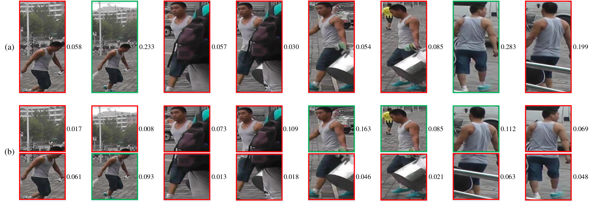
In this section, we first visualize the node scores learned by SAGPool [12] on a video sequence with 8 frames. We present the node scores of the global features and 2-nd order granularity features in Fig. 7. The nodes with top-2 scores and top-4 scores are retained for the global features and 2-nd order granularity features, respectively. From Fig. 7, we conclude that 1) features containing the occlusion would achieve the low scores; 2) features of the upper body are more important than the lower body.
5 Conclusions
To capture the temporal and spatial clues of the video-based ReID, we proposed the GPNet for the multi-granularity feature aggregation. We first formulated the input graphs with the multi-granularity features, where the edges were constructed for the both temporal and Euclidean neighborhood nodes; we then implemented the graph convolutional layers for the node neighborhood aggregation. To obtain the feature representation of the video sequence, we further adopted the graph pooling methods to decrease the number of nodes in graph, which was implemented by a multi-head full attention pooling method with fully considering the global cross-attention. Finally, we implemented the readout layer to obtain the fix-length representation of the pooled graph. We concatenated the multi-granularity graph representations as the video representation vector for the pedestrian retrieval. The experimental results on MARS, DukeMTMC-VideoReID and iLIDS-VID demonstrated the superiority of our GPNet.
Acknowledgment
This research is supported by the National Natural Science Foundation of China (Grant No.62172126 and Grant No.62106063), by the Shenzhen Research Council (Grant No. JCYJ20210324120202006), by the Shenzhen College Stability Support Plan (Grant GXWD20201230155427003-20200824113231001).
References
- [1] Y. Tang, X. Yang, et al., Person re-identification with feature pyramid optimization and gradual background suppression, Neural Networks 124 (2020) 223–232.
- [2] J. Wu, Y. Yang, et al., An end-to-end exemplar association for unsupervised person re-identification, Neural Networks 129 (2020) 43–54.
- [3] Y. Yang, T. Zhang, et al., Cross-modality paired-images generation and augmentation for rgb-infrared person re-identification, Neural Networks 128 (2020) 294–304.
- [4] A. Hermans, L. Beyer, B. Leibe, In defense of the triplet loss for person re-identification, arXiv preprint arXiv:1703.07737 (2017).
- [5] L. Zheng, Z. Bie, et al., Mars: A video benchmark for large-scale person re-identification, in: In Proceedings of the European Conference on Computer Vision, 2016, pp. 868–884.
- [6] X. Wang, R. Zhao, Person re-identification: System design and evaluation overview, in: Person Re-Identification, 2014, pp. 351–370.
- [7] J. Yang, W. Zheng, et al., Spatial-temporal graph convolutional network for video-based person re-identification, in: IEEE Conference on Computer Vision and Pattern Recognition, 2020, pp. 3289–3299.
- [8] W. Hamilton, R. Ying, J. Leskovec, Inductive representation learning on large graphs, in: Conference on Neural Information Processing Systems, 2017, pp. 1024–1034.
- [9] J. Gilmer, S. Schoenholz, et al., Neural message passing for quantum chemistry, in: International Conference on Machine Learning, 2017, pp. 1263–1272.
- [10] T. Kipf, M. Welling, Semi-supervised classification with graph convolutional networks, International Conference on Learning Representations (2017) 1–14.
- [11] R. Ying, J. You, et al., Hierarchical graph representation learning with differentiable pooling, in: Conference on Neural Information Processing Systems, 2018, pp. 4800–4810.
- [12] J. Lee, I. Lee, J. Kang, Self-attention graph pooling, in: International Conference on Machine Learning, 2019, pp. 3734–3743.
- [13] Y. Ma, S. Wang, et al., Graph convolutional networks with eigenpooling, in: Proceedings of the 25th ACM SIGKDD International Conference on Knowledge Discovery & Data Mining, 2019, pp. 723–731.
- [14] S. Wu, Y. Chen, et al., An enhanced deep feature representation for person re-identification, in: 2016 IEEE Winter Conference on Applications of Computer Vision, 2016, pp. 1–8.
- [15] T. Wang, S. Gong, et al., Person re-identification by video ranking, in: In Proceedings of the European Conference on Computer Vision, 2014, pp. 688–703.
- [16] M. Hirzer, C. Beleznai, et al., Person re-identification by descriptive and discriminative classification, in: Scandinavian conference on Image analysis, 2011, pp. 91–102.
- [17] M. Ye, J. Shen, et al., Deep learning for person re-identification: A survey and outlook, IEEE Transactions of Pattern Analysis and Machine Intelligence (2021).
- [18] Z. Zhong, L. Zheng, et al., Re-ranking person re-identification with k-reciprocal encoding, in: IEEE Conference on Computer Vision and Pattern Recognition, 2017, pp. 1318–1327.
- [19] H. Luo, Y. Gu, et al., Bag of tricks and a strong baseline for deep person re-identification, in: IEEE Conference on Computer Vision and Pattern Recognition Workshops, 2019.
- [20] G. Wang, Y. Yuan, et al., Learning discriminative features with multiple granularities for person re-identification, in: Proceedings of the 26th ACM International Conference on Multimedia, 2018, pp. 274–282.
- [21] Y. Sun, L. Zheng, et al., Beyond part models: Person retrieval with refined part pooling (and a strong vonvolutional baseline), in: In Proceedings of the European Conference on Computer Vision, 2018, pp. 480–496.
- [22] Y. Suh, J. Wang, et al., Part-aligned bilinear representations for person re-identification, in: In Proceedings of the European Conference on Computer Vision, 2018, pp. 402–419.
- [23] C. Su, S. Zhang, et al., Deep attributes driven multi-camera person re-identification, in: In Proceedings of the European Conference on Computer Vision, 2016, pp. 475–491.
- [24] Y. Zhao, X. Shen, et al., Attribute-driven feature disentangling and temporal aggregation for video person re-identification, in: IEEE Conference on Computer Vision and Pattern Recognition, 2019, pp. 4913–4922.
- [25] F. Schroff, D. Kalenichenko, J. Philbin, Facenet: A unified embedding for face recognition and clustering, in: IEEE Conference on Computer Vision and Pattern Recognition, 2015, pp. 815–823.
- [26] Y. Wen, K. Zhang, et al., A discriminative feature learning approach for deep face recognition, in: In Proceedings of the European Conference on Computer Vision, 2016, pp. 499–515.
- [27] W. Wang, W. Pei, et al., Push for center learning via orthogonalization and subspace masking for person re-identification, IEEE Transactions on Image Processing 30 (2020) 907–920.
- [28] C. Wang, Q. Zhang, et al., Mancs: A multi-task attentional network with curriculum sampling for person re-identification, in: In Proceedings of the European Conference on Computer Vision, 2018, pp. 365–381.
- [29] D. Chen, H. Li, et al., Video person re-identification with competitive snippet-similarity aggregation and co-attentive snippet embedding, in: IEEE Conference on Computer Vision and Pattern Recognition, 2018, pp. 1169–1178.
- [30] D. Chung, K. Tahboub, E. Delp, A two stream siamese convolutional neural network for person re-identification, in: IEEE International Conference on Computer Vision, 2017, pp. 1983–1991.
- [31] X. Gu, H. Chang, et al., Appearance-preserving 3d convolution for video-based person re-identification, in: In Proceedings of the European Conference on Computer Vision, Springer, 2020, pp. 228–243.
- [32] J. Li, S. Zhang, T. Huang, Multi-scale 3d convolution network for video based person re-identification, in: Proceedings of the AAAI Conference on Artificial Intelligence, Vol. 33, 2019, pp. 8618–8625.
- [33] N. McLaughlin, J. Martinez, P. Miller, Recurrent convolutional network for video-based person re-identification, in: IEEE Conference on Computer Vision and Pattern Recognition, 2016, pp. 1325–1334.
- [34] Y. Yan, B. Ni, et al., Person re-identification via recurrent feature aggregation, in: In Proceedings of the European Conference on Computer Vision, 2016, pp. 701–716.
- [35] A. Subramaniam, A. Nambiar, A. Mittal, Co-segmentation inspired attention networks for video-based person re-identification, in: IEEE Conference on Computer Vision and Pattern Recognition, 2019, pp. 562–572.
- [36] Z. Zhang, C. Lan, et al., Multi-granularity reference-aided attentive feature aggregation for video-based person re-identification, in: IEEE Conference on Computer Vision and Pattern Recognition, 2020, pp. 10407–10416.
- [37] C. Liu, C. Wu, et al., Spatially and temporally efficient non-local attention network for nideo-based person re-identification, arXiv preprint arXiv:1908.01683 (2019).
- [38] Y. Yan, J. Qin, et al., Learning multi-granular hypergraphs for video-based person re-identification, in: IEEE Conference on Computer Vision and Pattern Recognition, 2020, pp. 2899–2908.
- [39] J. Bruna, W. Zaremba, et al., Spectral networks and locally connected networks on graphs, in: International Conference on Learning Representations, 2014, pp. 1–14.
- [40] M. Defferrard, X. Bresson, P. Gheynst, Convolutional neural networks on graphs with fast localized spectral filtering, in: Conference on Neural Information Processing Systems, 2016, pp. 3844–3852.
- [41] F. Bianchi, G. D, C. Alippi, Spectral clustering with graph neural networks for graph pooling, in: IEEE International Conference on Computer Vision, 2020, pp. 874–883.
- [42] H. Gao, S. Ji, Graph u-nets, in: International Conference on Machine Learning, 2019, pp. 2083–2092.
- [43] K. He, X. Zhang, et al., Deep residual learning for image recognition, in: IEEE Conference on Computer Vision and Pattern Recognition, 2016, pp. 770–778.
- [44] X. Wang, R. Girshick, et al., Non-local neural networks, in: IEEE Conference on Computer Vision and Pattern Recognition, 2018, pp. 7794–7803.
- [45] D. Kingma, J. Ba, Adam: A method for stochastic optimization, arXiv preprint arXiv:1412.6980 (2014).
- [46] Q. Li, Z. Han, X. Wu, Deeper insights into graph convolutional networks for semi-supervised learning, in: Proceedings of the AAAI Conference on Artificial Intelligence, Vol. 32, 2018.
- [47] R. Hou, B. Ma, et al., Vrstc: Occlusion-free video person re-identification, in: IEEE Conference on Computer Vision and Pattern Recognition, 2019, pp. 7183–7192.
- [48] J. Li, J. Wang, et al., Global-local temporal representations for video person re-identification, in: IEEE International Conference on Computer Vision, 2019, pp. 3958–3967.
- [49] R. Hou, H. Chang, et al., Temporal complementary learning for video person re-identification, in: In Proceedings of the European Conference on Computer Vision, 2020, pp. 388–405.
- [50] G. Chen, Y. Rao, et al., Temporal coherence or temporal motion: Which is more critical for video-based person re-identification?, in: In Proceedings of the European Conference on Computer Vision, 2020, pp. 660–676.
- [51] X. Jiang, Y. Qiao, et al., Ssn3d: Self-separated network to align parts for 3d convolution in video person re-identification, in: Proceedings of the AAAI Conference on Artificial Intelligence, Vol. 35, 2021, pp. 1691–1699.
- [52] X. Liu, P. Zhang, et al., Watching you: Global-guided reciprocal learning for video-based person re-identification, in: IEEE Conference on Computer Vision and Pattern Recognition, 2021, pp. 13334–13343.
- [53] R. Hou, H. Chang, et al., Bicnet-tks: Learning efficient spatial-temporal representation for video person re-identification, in: IEEE Conference on Computer Vision and Pattern Recognition, 2021, pp. 2014–2023.