Colliding gravitational waves and singularitiesPreprint: YITP-22-102
Abstract
We have investigated a model of colliding plain gravitational waves, proposed by Szekeres, whose structure of singularities is determined. We have evaluated a total energy of matter as a volume integral of the energy momentum tensor (EMT), whose contributions arise only at these singularities. The total matter energy is conserved before a collision of two plane gravitational waves but decreases during the collision and becomes zero at the end of the collision. We thus interpret that this model of colliding plane gravitational waves is a spacetime describing a pair annihilation of plan gravitational waves. We have also calculated a matter conserved charge proposed by the present author and his collaborators. The matter charge is indeed conserved but is zero due to a cancellation between two plain gravitational waves. This seems natural since nothing remains after a pair annihilation, and give a hint on a physical interpretation of the conserved charge, which we call the gravitational charge. By modifying the space time for the pair annihilation, we newly construct two types of a scattering plane gravitational wave and a pair creation of plane gravitational waves, and combining all, a Minkowski vacuum bottle, a Minkowski spacetime surrounded by two moving plane gravitational waves.
1 Introduction
Is a total energy always conserved in general relativity ? To answer this question theoretically is rather non-trivial. Usually in a flat spacetime, as a consequence of Noether’s (first) theorem for a global symmetryNoether:1918zz, a time translation symmetry of a system defines a corresponding energy density as the time component of the Noether current, and also tells us that a total energy given by a volume integral of the energy density is conserved. This construction of a conserved energy does not work in general relativity, however, since a time translational symmetry is a part of local symmetries, general coordinate transformations, to which Noether’s first theorem can not be applied. Indeed, Noether’s second theoremNoether:1918zz tells us that, instead of dynamically conserved currents, there exist non-trivial constraints in a theory with local symmetries such as Bianchi identity or Gauss law constraint. Related but not equivalent to this problem, a conservation of the energy momentum tensor (EMT) in general relativity, does not directly give a conserved energy or momentum due to non-linear terms in covariant derivatives. There have been several proposals for a definition of energy in general relativity, which may be categorized into two types. One is Einstein’s pseudo-tensor definition, and the other is a quasi-local definition including Komar energyKomar:1958wp or ADM energyArnowitt:1962hi. Since both definitions correspond to some constraints implied by Noether’s second theoremAoki:2022gez, it is easy to show that their current densities are always conserved without using equations of motion, and moreover, the corresponding total energy can be always written as a surface integral rather than a volume integral via Stoke’s theorem.
Recently, the present author, together with his collaborators, has proposed an alternative definition for energy in general relativityAoki:2020prb; Aoki:2020nzm without using constraints from Noether’s second theorem. In a case that a stationary Killing vector exists, the energy defined from the EMT11 1 In this case, this energy agrees with the one proposed in Ref. Fock1959. correctly reproduces the known mass of the Schwarzschild black hole, and the mass and the angular momentum of the BTZ black holeAoki:2020prb. For a spherically symmetric compact star, on the other hand, the energy in our definition is different from the corresponding ADM mass, and its difference may be interpreted as a positive contribution of gravitational fields to the ADM mass. Even in the absence of the stationary Killing vector, the energy is shown to be conserved during some types of gravitational collapsesAoki:2020nzm; Yokoyama:2021nnw. Since the energy is defined from the EMT of matters, we may call it a ‘‘matter energy” hereafter. In general, however, the matter energy is not conserved, so that an answer to the question in the beginning is ‘‘No.”. Although the matter energy is not conserved, one can still define a more general conserved charge associated with the EMT in general relativity,22 2 This definition is a generalization of the conserved charge proposed for a spherically symmetric spacetime in Ref. Kodama:1979vn. which behaves like “entropy” for special cases such as homogeneous and isotropic expanding universeAoki:2020nzm.
In this paper, we apply the definition of matter energy and its generalization in general relativity to a non-trivial dynamical processes that two plane gravitational waves collides with each other and become a black hole-like object, which is a vacuum solution to the Einstein equation except singularities. (See Refs. Szekeres:1972uu; Khan:1971vh; Yurtsever:1988ks; Yurtsever:1988vc for early analytic studies on this type of processes.) We exclusively consider a model of colliding plane gravitational waves proposed by SzekeresSzekeres:1972uu, which gives a simple analytic solution to the vacuum Einstein equation with some singularities. Although it turns out that singularities after the collision is not a black hole but something similar, this model is still suitable to check whether our proposal for matter energy and its generalization works well even for this complicated dynamical processes. In Sec. 2, we explain the model in detail and determine a spacetime structure including singularities. We then calculate the total matter energy of the system in Sec. 3, as a volume integral of the EMT, whose non-zero contributions comes form its singularities. It turns out that the total matter energy is not conserved during the collision, though it is conserved before the collision. On the other hand, the generalized matter charge, which we call the gravitational charge, can be defined so as to be conserved but is found to be zero by a cancellation between two contributions. Indeed a geometry of the Szekeres’ model is found to describe a pair annihilation of two plane gravitation waves at a certain time, when a total matter energy also becomes zero. The vanishing gravitational charge is consistent with this geometry. In Sec. 4, modifying a geometry of the colliding two gravitational waves, we construct several new spacetime geometries, which are two types of a scattering plane gravitational wave, and a creation of two plane gravitational wave from nothing. Combining all four, a pair creation of two plane gravitational wave, a scattering of each plane gravitational wave, and a pair annihilation of them, we finally construct a geometry, named “Minkowski vacuum bottle”, a Minkowski spacetime surrounded by two plane gravitational waves. Our conclusions, together with some discussions, are given in Sec. 5. In appendix A, we evaluate the generalized Komar integral as a representative of quasi-local definitions of energy for the the Szekeres’ model for a comparison.
2 Colliding plane gravitational waves
2.1 Setup
We consider colliding plane gravitational waves, investigated by SzekeresSzekeres:1972uu, whose metric is given by
| (1) |
where and are light-cone coordinate. In a flat spacetime, corresponds to a time, while denotes a spacial position in the Cartesian coordinate. The vacuum Einstein equation reads
| (2) | |||||
| (3) | |||||
| (4) | |||||
| (5) | |||||
| (6) |
where subscript represent derivatives with respect to them.
2.2 Solutions to the vacuum Einstein equation
Ref. Szekeres:1972uu has solved the above Einstein equations in the 4 regions defined by
- I.
Minkowski spacetime at and .
- II.
A left moving plane wave at and .
- III.
A right moving plane wave at and .
- IV.
Colliding two plane waves at and .
A class of the explicit solutions is given bySzekeres:1972uu
| (7) |
where
| (8) | |||||
| (9) |
, and are related to even integers as
| (10) |
These relations lead to
| (11) |
Thanks to functions in (9), these solutions hold in all regions. As a continuity of the metric and its first derivative, the strongest requirements become
| (12) |
at the I-II boundary (), and
| (13) |
at the I-III boundary (), which leads to and for even integers . Other conditions that , at and , at are automatically satisfied. Note that these continuity conditions exclude two colliding impulse wavesKhan:1971vh and two colliding sandwich plane wavesYurtsever:1988ks; Yurtsever:1988vc, both of which have .
2.3 Singularities
In the region IV, the Riemann curvature invariant shows a singular behavior at as
| (14) | |||||
at , while the invariant identically vanishes in other regions.
In regions II and III, Riemann tensors and Weyl tensors have singularitiesSzekeres:1972uu, which are indeed physical, not coordinate singularities as shown below. In the region II, the metric in (1) can be transformed to the Brinkmann coordinateBrinkmann:1923cd as
| (19) |
through the coordinate transformation defined by
| (20) |
where
| (21) |
and are only non-zero components of the Riemann tensor in this coordinate. Explicitly, we obtain
| (22) |
which is regular at for , but singular at as with . Similarly
| (23) |
in the region III. According to Ref. Blau:2011ab, singularities in (22) and (23) at are physical for plane waves in the regions II and III.
In summary, the metric in (1) has singularities at in region II, III and IV.
2.4 Apparent horizon
Since there are singularities at , we determine locations of apparent horizons if exist. For this purpose, we calculate an expansion for an affinely parametrized null geodesic33 3 We here use instead of to represent the expansion, in order to avoid a confusion with the step function . , defined by , where is the tangent vector of the affinely parametrized null geodesic satisfying and . The apparent horizon (AH) is determined by the condition that changes its sign. Since it is easy to see that in the region I (flat spacetime), there is no AH in the region I as it should be.
In the region II, two tangent vectors for future directed null geodesics are given by
| (24) |
Corresponding expansions are calculated as
| (25) |
Since at and at , we identify a boundary between I and II at as the apparent horizon. Note that, even though does not becomes positive but stay zero at , we here extend a meaning of apparent horizon as a boundary between and regions.
Similarly in the region III, we have
| (26) |
for and , so that the apparent horizon appears at ( a boundary between I and III).
In the region IV, we take and , which lead to
| (27) |
where
| (28) |
Thus the AH appears at (a boundary between II and IV) for and at (a boundary between III and IV) for .
2.5 Global spacetime structure
Fig. 1 gives a rough sketch of a spacetime defined by the metric (1), which exist only at and is bounded by singularities at (a red line in the figure) as
| (29) |
while apparent horizons appears at with and at with (magenta lines in the figure). This spacetime is very similar to the one for two colliding impulse wavesKhan:1971vh except that function singularities in the curvature appear at and for two colliding impulse wavesKhan:1971vh, instead of the apparent horizons mentioned above.
3 Matter energy and generalized matter conserved charge
3.1 Energy momentum tensor at singularities
A matter energy is evaluated by a volume integral of the EMT at a give as
where with Newton constant . While is zero except singularities, this integral becomes non-zero due to contributions from singularities of . In order calculate this type of the integral, it is convenient to express or in terms of delta functions, which represent contributions from singularities to the integral, as in the case of black holesBalasin:1993fn; Balasin:1993kf; Kawai:1997jx; Aoki:2020prb.
In order to evaluate a contribution of the EMT in the volume integral, we first regularize singularities by modifying in the metric as
| (30) |
where
| (31) |
with an infinitesimally small but non-zero real constant , and real constants . In the limit, we recover (7). The regularization of makes all components of Riemann tensor finite at , so that we can extend the space time to the region. As a result, there may appear other singularities at or in the region IV in the region. This is a reason why we also have to regularize and by and for the extension of spacetime to the region. Note that the integral of the EMT tensor in the physical region does not depend on a choice of regularizations after the regularization is removed, as will be seen later.
With non-zero , the metric is no more a vacuum solution, giving non-zero EMT as
| (32) | |||||
| (33) | |||||
| (34) | |||||
| (35) |
where extra terms are evaluated for small as
| (36) | |||||
| (37) | |||||
| (38) | |||||
| (39) |
Since
and
| (43) |
we can write
| (44) |
in the physical region at . Although the explicit form of in (31) is used to derive (44), one can obtain the same result from a different form of the regularization as long as satisfies (3.1) and (43):
A non-physical region at beyond singularities gives an extra contribution in this regularization as
| (48) |
which does not affect the integral of the EMT in the physical region at . An extra contribution depends on how we extend the metric into the region. For example, if we take
where and are continuous, an integral in each region becomes
| (52) |
so that an extra contribution from the region vanishes. More generally, if we take
where a function satisfies
| (56) |
the contribution from the non-physical region to the integral becomes
| (57) |
Thus, after removing the regularization, the contribution from the non-physical region becomes , which can be arbitrary by a freedom of . Since the physical spacetime at is separated from the non-physical one at by singularities at , this arbitrariness of the regularization at does not affect integrals of the EMT in the physical region at .
We can also show that extra contributions form all vanish in the physical region after the limit, since
| (58) |
We then finally obtain
| (59) |
in the limit for the original spacetime at .
In order to see that the same result (59) can be obtained by a simpler regularization Aoki:2020prb as , since
| (60) |
where we use and . This agreement again demonstrates that the result (59) is universal.
A relation give an expression of the EMT in terms of delta functions. While singularities are light-like in regions II and III, singularities in the region IV are space-like, as in the case of the Schwarzschild blackhole.
3.2 Energy non-conservation
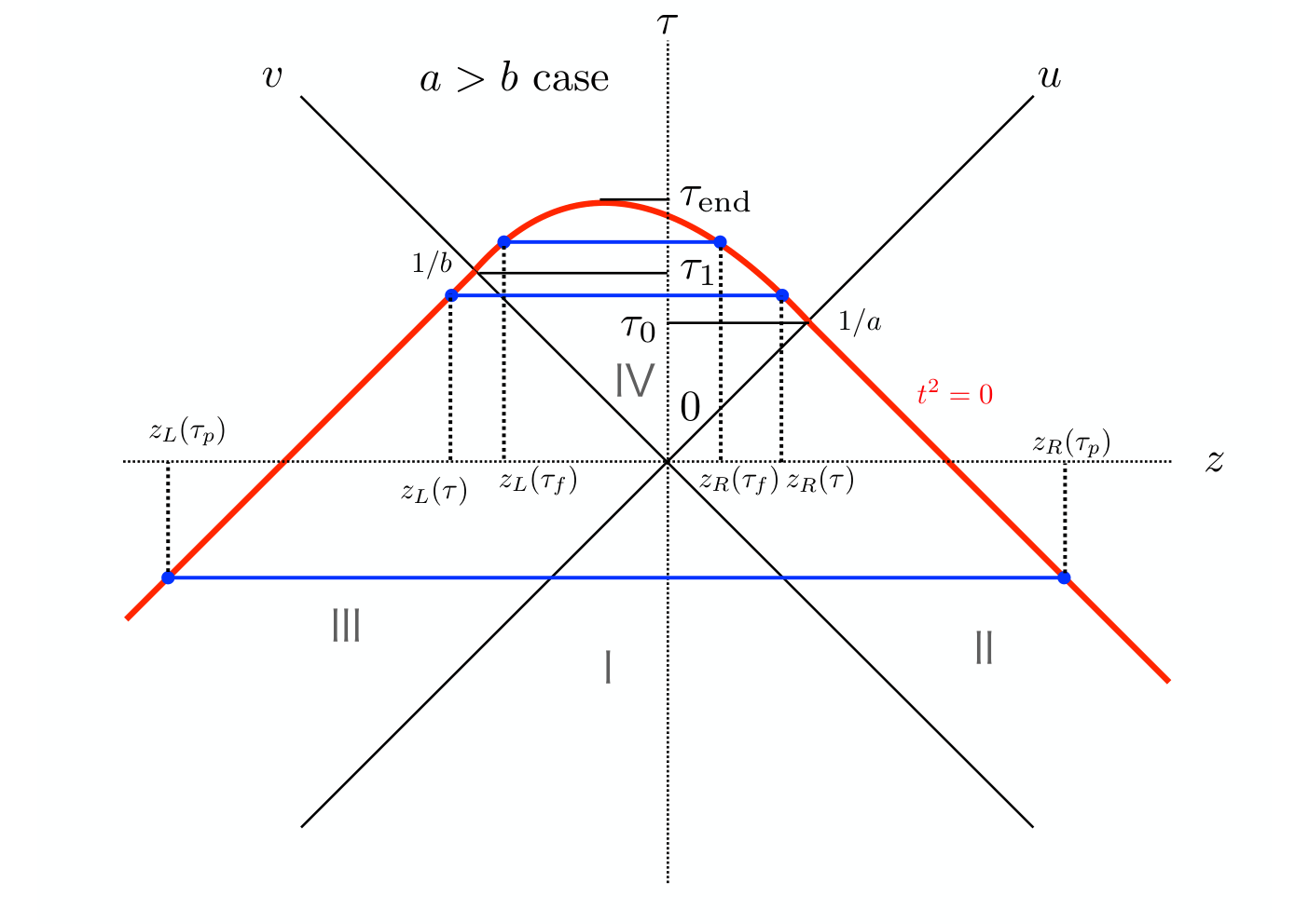
Since the spacetime is uniform in and directions, we define the matter energy of the system per unit 2-dimensional volume for a given from with Aoki:2020nzm; Aoki:2020prb as
| (61) | |||||
where is a 2-dimensional volume, which diverges in infinite 2-dimensional extensions. The energy defined in the above depends on the choice of the time coordinate , as in the case of the flat Minkowski space time, where the energy also depends on the choice of the time coordinate and it transforms as a vector under Poincare transformation.
In general, has two solutions at a given in this spacetime, larger of which is denoted by and smaller by , so that at and at . Since
| (62) |
at while at . At a given , the space exists only in an interval . Positions of depend on a value of , as shown in Fig. 2 for and explained below.
- 1.
, where . In this case, in the region II, while at in the region III. In Fig. 2, and belong to this case.
- 2.
, where . For , is a solution to with and for a given in the region IV and is a solution of in the region III. In Fig. 2, and belong to this case. On the other hand, for , is a solution of in the region II and is a solution to for a given in the region IV.
- 3.
, where is a solution to the following equations
(63) Thus . In a simple case that , we have
(64) In this range of , are two solutions to in the region IV. In Fig. 2, and belong to this case.
Using the above property, energy can be evaluated as follows. At , we have
| (65) |
At , we have
Since for , or for , in (3.2)
decreases from (65). Thus the energy is not conserved in this spacetime.
At , we finally obtain
| (70) |
which is further decreasing, and vanishes at when the space in the direction disappear as . Therefore the time is a moment for an end of the universe, when all matters also should disappear to be consistent with .
3.3 Conserved charge
Even though the matter energy is not conserved, we can construct a non-trivial conserved charge from a conserved current as , where a vector must satisfy Aoki:2020nzm; Aoki:2022gez. In this construction, however, there are so many different choices for a direction of the vector . In this paper, we propose an unique method to determine up to an initial condition.
We first decompose the EMT as
| (71) |
where ellipses represents components, which we do not consider in this section, and vectors and are given by
| (72) |
in the coordinate.
Our new proposal is to take , which is determined by the EMT, thus is coordinate independent. Explicitly, we take
| (73) |
in the region IV, where . Then the conserved current density becomes
| (74) |
which can be used even in regions II and III.
Since we require , must satisfies
| (75) |
whose general solution is given by
| (76) |
where is an arbitrary differentiable function.
The corresponding conserved charge per is defined by
The conservation of is derived from an integral of over a space-time region in the plane surrounded by 4 boundaries, , , , and , as shown in Fig. 2. Therefore, we need to check that boundary contributions on and vanish to establish the conservation of . Since the (unnormalized) normal vector to the singularity surface is given by , integrands in boundary contributions along the singularity surface always vanish as
| (78) |
so that for arbitrary .
The charge at all can be explicitly calculated as
| (79) |
which vanishes due to a cancelation between a contribution at and a contribution at , except where a contribution identically vanishes at . The charge is indeed conserved.
We thus conclude that there exists a conserved charge in the spacetime given by (1), whose value is zero by the cancellation of two contributions. A fact that in this spacetime seems natural, since the spacetime ceases to exist at , when all matters should disappear, so that . If is conserved unlike energy , must hold for all .
In Aoki:2020nzm; Aoki:2022gez, analysis for some particular spacetimes with matters described by a perfect fluid indicated that a generic matter conserved charge in general relativity may be interpreted as a matter entropy. Since can be locally negative in the metric (1), however, we may need to reconsider a physical interpretation of the matter conserved charge once more. We may call a gravitational charge, which is more general and becomes the matter entropy only for special cases. The gravitational charge may be locally negative in the special spacetime described by (1), which ceases to exist at and whose singularities in the region IV are superluminal. Further investigations will be required to distinguish one possibility from the other.
4 Construction of new spacetimes
Motivated by the geometry of colliding plane gravitational waves, we construct other types of the plane wave(s) in this section. Since and are even integers, and in (7) and (8) satisfy the vacuum Einstein equation in all regions, where
| (80) |
We can construct new solutions by putting functions to appropriate places, in order to satisfy boundary conditions at and .
4.1 A scattering of the plane gravitational wave
The first example is a scattering of the plane gravitational wave.
The left-moving gravitational wave in the region II is scattered in the region IV, and then it appears as the right-moving gravitational wave in the region III, as shown in Fig. 3 (Left), while the right-moving gravitational wave in the region III, scattered in the region IV, goes into the region II as the left-moving wave, as shown in Fig. 3 (Right). Solutions for both cases are given by (7) with
| (81) |
for the left-to-right scattering, and
| (82) |
for the right-to-left scattering. Note that singularities at (red line) are either time-like in the region IV or light-like in regions II and III.
Let us calculate the matter energy using the definition as
| (83) |
The matter energy for the left-to-right scattering in Fig. 3 (Left) becomes
| (84) |
at (the region II), and
| (85) |
at (the region III). In the region IV at , we have
| (86) |
Therefore the matter energy is constant in the region II as well as the region III, while is decreasing or increasing in the region IV if or , respectively.
Similarly, the matter energy for the right-to-left scattering in Fig. 3 (Right) is given by
where and . Again the matter energy is constant in the regions III and II, while is decreasing or increasing in the region IV for or , respectively.
We next consider the matter conserved charged, given by
| (93) |
In the case of the left-to-right scattering, we obtain
| (94) |
while we have
| (95) |
for the right-to-left scattering, where and are arbitrary constants given by . Therefore the matter conserved charge is non-zero and conserved for these scatterings.
4.2 Pair creation of gravitational waves
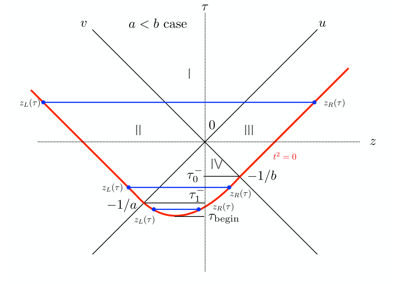
As a time reversal process to the colliding plane gravitational waves, we consider a creation of left and right moving plane gravitational waves, as illustrated in Fig. 4, where a pair creation occurs at in the region IV.
With functions and , is determined from and which satisfy
| (96) |
For a special case that , we obtain
| (97) |
At , the matter energy at in this range is given by
| (98) |
which increases from as increases, where and are smaller and larger solutions to in the region IV, respectively.
At , we have
which is still increasing, since and .
Finally the matter energy becomes largest at , and stays constant at as
| (103) |
As in the case of the colliding plane gravitational wave, the matter conserved charge at all vanishes as
| (104) | |||||
4.3 Minkowski vacuum bottle
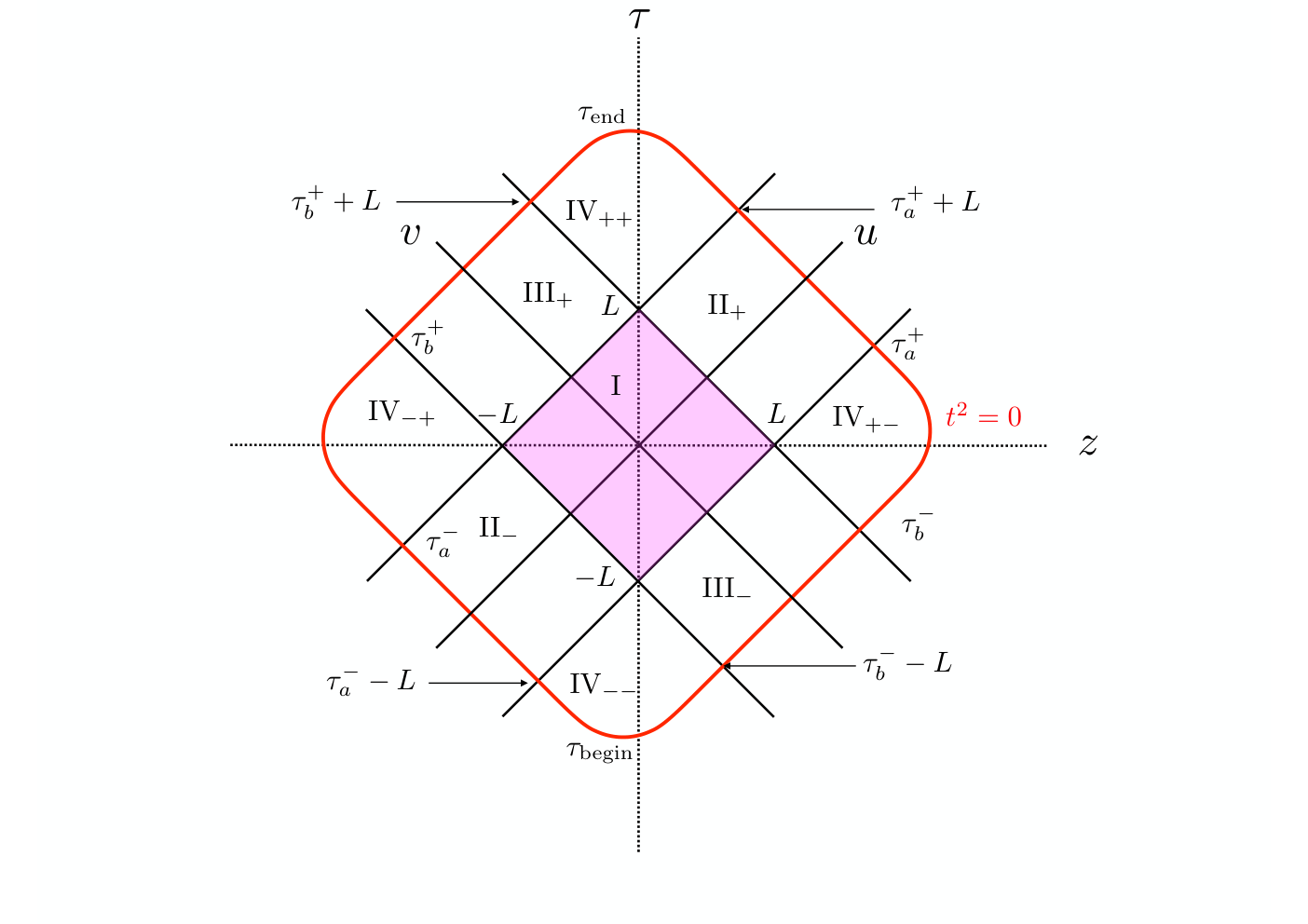
We can assemble all four spacetimes: two gravitational waves are created at , then the left-moving wave is scattered to the right-moving and vice versa, and two waves collides and finally annihilate at , as illustrated in Fig. 5, where there are 9 regions denoted by I, II±, III±, IV±± and IV±∓.
To specify these regions, we need 4 functions, and , defined by
| (105) |
where
| (106) |
and is a diagonal length of the squire region I in the middle, whose center is . A function corresponds to a region IIα, while corresponds to a region IIIβ. On the other hand, a pair of function are used to specify a region IVαβ.
During the time evolution, the matter energy first increase from , then decreases and vanishes at , where and satisfies with and with , respectively. Note that energy sometimes stays constant for a while during this process.
Explicitly we have , where and are energies of the left-to-right moving wave and the right-to-left moving one, respectively, which are given by
Here and are smaller and larger solutions to at a given for take . See some time coordinates in Fig. 5.
The matter conserved charge is always zero by a cancellation between the left-to-right moving wave and the right-to-left moving wave, as seen from (79), (104), and (94) (95) with .
It is interesting to see that the Minkowski vacuum appears in the center of this spacetime ( the region I in magenta) surrounded by two moving plane gravitational waves with matters at singularities. Thus we call this spacetime a ”Minkowski vacuum bottle”. The region I is separated from others by apparent horizons, and begins at , expands until , then contracts and finally disappears at .
5 Conclusions and Discussions
In this paper, we have analyzed a model of colliding plain gravitational waves, proposed by Szekeres Szekeres:1972uu. A structure of singularities in the spacetime is determined, and then contributions from the energy momentum tensor (EMT) at these singularities are determined through the Einstein equation. We have evaluated the total energy of the matter as a volume integral of the EMTAoki:2020prb; Aoki:2020nzm, which is conserved before the collision of two plane gravitational waves but decreases during the collision and becomes zero at the end of the collision. Thus the model of colliding plain gravitational waves can be regarded as a spacetime describing a pair annihilation of plain gravitational waves. We have also evaluated the gravitational charge as the generalized matter conserved charge proposed in Ref. Aoki:2020nzm. The gravitational charge is indeed conserved but is zero due to a cancellation of contributions between two plain gravitational waves. The vanishing conserved charge seems natural since nothing remains after a pair annihilation of plain gravitational waves. While the gravitational charge can be interpreted as the entropy in Ref. Aoki:2020nzm for special cases, our result in this paper that it can become locally negative may suggest that the gravitational charge is more general than the entropy. We leave this problem to future studies. It is also interesting to apply the analysis in this paper to other models of colliding gravitational waves such as Alcubierre:1999ex; Pretorius:2018lfb, for example.
By modifying the spacetime for a pair annihilation of plain gravitational waves, we construct two types of a scattering plane gravitational wave as well as a pair creation of plain gravitational waves. Combining all, we also create a Minkowski vacuum bottle, a Minkowski spacetime surrounded by two moving plane gravitational waves with singularities. The total matter energy as well as the conserved gravitational charge are calculated in each case. As expected, while the matter energy is not conserved, the gravitational charge is indeed conserved.
According to the proposal in Ref. Aoki:2020prb; Aoki:2020nzm, an answer to the question in the beginning of the introduction that ”Is a total energy always conserved in general relativity ? ” may be answered as follow. In general relativity, the total energy of the matter can be defined but is not conserved in general. However there always exists a conserved gravitational charged as a matter conserved charge. In this paper we have shown that these statements hold for the colliding plain gravitational waves and their variants. The above answer, however, seems unsatisfactory, since one may hope that the total energy including both matter energy and gravitational energy is conserved in general relativity. Unfortunately, it is not easy to define the gravitational energy and thus the conserved total energy in general relativity. One may say that the conserved current of the Noether’s 2nd theorem can be used to define the total energy in general relativity. This, however, may not be the final answer since the conservation via the Noether’s 2nd theorem is not dynamicalNoether:1918zz; Aoki:2022gez; Deriglazov:2017biu. As an evidence to support this statement, we show in appendix A that the generalized Komar integralKomar:1958wp, which is a generic conserved charge from the Noether’s 2nd theorem and is regarded as a representative for the quasi-local energy, is not conserved for the colliding plane gravitational waves. This suggests that the generalized Komar integral is physically an improper definition of “energy”, as has been pointed out beforeMisner:1963zz. To find a conserved total energy including contributions from gravitational fields will be the next important task in our future studies, even though such a concept may not exist in general relativity.
Acknowledgment
The author would like to thank Mr. Takumi Hayashi , Drs. Ryo Namba, Naritaka Oshita and Daisuke Yoshida for useful discussions and valuable comments, and give his special thanks to Mr. Takumi Hayashi for his contributions, who provided the result in eq. (14) by Mathematica before the author’s analytic calculation. This work is supported in part by the Grant-in-Aid of the Japanese Ministry of Education, Sciences and Technology, Sports and Culture (MEXT) for Scientific Research (Nos. JP22H00129).
Appendix A Generalized Komar integral for colliding plane gravitational waves
In this appendix, we evaluate a Komar-type integralKomar:1958wp for the colliding plane gravitational waves, since it, together with its variants, covers large varieties of quasi-local definitions of “energy” in general relativity.
The Komar current44 4 The Komar energy is originally defined by in the case that is a time-like Killing vector. Since is always conserved, we here define the Komar energy for an arbitrary vector , which we call the generalized Komar integral. is given by
| (127) |
whose covariant divergence identically vanishes as for an arbitrary vector without using equations of motion, as a consequence of Noether’s 2nd theoremAoki:2022gez. Therefore an identity,
| (128) |
holds for an arbitrary space-time region with a boundary . Taking a region in the plane surrounded by 4 boundaries, , , and (See an example in Fig. 2), we obtain a relation that
| (129) |
where
| (130) |
Therefore, the generalized Komar integral is -independent (i.e. conserved), if for .
Using the Stokes theorem and performing trivial integrals, we write
| (131) |
where
| (132) |
In the following analysis, we take and , so that
| (133) |
where
| (134) |
at . We thus obtain
| (135) | |||||
| (136) |
both of which vanish for and , so that the generalized Komar integral is conserved trivially and becomes zero in this case.
We thus consider a more non-trivial case that and with constants , and take , at which we have
| (137) |
Note that agrees with the energy of two plane gravitational waves before collision, eq. (65), if we take .
Let us consider the following 3 cases for separately.
- 1.
: In this case, the energy is conserved as . Indeed we also confirm .
- 2.
: In this case
where and for . Since , the generalized Komar integral is not conserved. Indeed is satisfied, where
(142) (143) - 3.
: In this case
(144) The generalized Komar integral is not conserved as , where
(145) (146) Note that since and .
Let us conclude that, while the Komar current is always conserved locally, the generalized Komar integral is not conserved in general, due to non-zero contributions from integrals on other boundaries, .
It is worth mentioning that, as discussed in the main text, integrals of on boundaries at are always zero, since on these boundaries. This is not an accidental, as any matters never flow into regions outside the defined spacetime. If some matter exists, the corresponding spacetime must also exist according to Einstein equation. On the other hand, this argument can not be applied to the Komar current since it does not have such a physical meaning, so that a conservation of the generalized Komar integral is not automatically guaranteed in general, as seen in this appendix.
References
- (1) E. Noether, Gott. Nachr. 1918 (1918), 235-257 doi:10.1080/00411457108231446 [arXiv:physics/0503066 [physics]].
- (2) A. Komar, Phys. Rev. 113 (1959), 934-936 doi:10.1103/PhysRev.113.934
- (3) R. L. Arnowitt, S. Deser and C. W. Misner, in Gravitaion: an introduction to current research, L. Witten, ed. (Wiley, New York, 1962). See also Gen. Rel. Grav. 40, 1997-2027 (2008) doi:10.1007/s10714-008-0661-1.
- (4) S. Aoki and T. Onogi, Int. J. Mod. Phys. A 37 (2022) no.22, 2250129 doi:10.1142/S0217751X22501299 [arXiv:2201.09557 [hep-th]].
- (5) S. Aoki, T. Onogi and S. Yokoyama, Int. J. Mod. Phys. A 36 (2021) no.10, 2150098 doi:10.1142/S0217751X21500986 [arXiv:2005.13233 [gr-qc]].
- (6) S. Aoki, T. Onogi and S. Yokoyama, Int. J. Mod. Phys. A 36 (2021) no.29, 2150201 doi:10.1142/S0217751X21502018 [arXiv:2010.07660 [gr-qc]].
- (7) V. Fock, Theory of Space, Time, and Gravitation (Pergamon Press, New York, 1959)
- (8) S. Yokoyama, [arXiv:2105.09676 [gr-qc]].
- (9) H. Kodama, Prog. Theor. Phys. 63 (1980), 1217 doi:10.1143/PTP.63.1217
- (10) P. Szekeres, J. Math. Phys. 13 (1972), 286-294 doi:10.1063/1.1665972
- (11) K. A. Khan and R. Penrose, Nature 229 (1971), 185-186 doi:10.1038/229185a0
- (12) U. Yurtsever, Phys. Rev. D 37 (1988), 2803-2817 doi:10.1103/PhysRevD.37.2803
- (13) U. Yurtsever, Phys. Rev. D 38 (1988), 1706-1730 doi:10.1103/PhysRevD.38.1706
- (14) H. Balasin and H. Nachbagauer, Class. Quant. Grav. 10, 2271 (1993) doi:10.1088/0264-9381/10/11/010 [arXiv:gr-qc/9305009 [gr-qc]].
- (15) H. Balasin and H. Nachbagauer, Class. Quant. Grav. 11, 1453-1462 (1994) doi:10.1088/0264-9381/11/6/010 [arXiv:gr-qc/9312028 [gr-qc]].
- (16) T. Kawai and E. Sakane, Prog. Theor. Phys. 98 (1997), 69-86 doi:10.1143/PTP.98.69 [arXiv:gr-qc/9707029 [gr-qc]].
- (17) H.W. Brinkmann, Proc. US Nat. Acad. Sci. 9 (1923) 1.
- (18) Matthias Blau, “Plane waves and Penrose limits”, Lecture note (November 15, 2011), http://www.blau.itp.unibe.ch/Lecturenote.html
- (19) A. Deriglazov, Sect. 8.8.2 in “Classical Mechanics: Hamiltonian and Lagrangian Formalism,” (doi:10.1007/978-3-319-44147-4).
- (20) M. Alcubierre, G. Allen, B. Bruegmann, G. Lanfermann, E. Seidel, W. M. Suen and M. Tobias, Phys. Rev. D 61 (2000), 041501 doi:10.1103/PhysRevD.61.041501 [arXiv:gr-qc/9904013 [gr-qc]].
- (21) F. Pretorius and W. E. East, Phys. Rev. D 98 (2018) no.8, 084053 doi:10.1103/PhysRevD.98.084053 [arXiv:1807.11562 [gr-qc]].
- (22) C. W. Misner, Phys. Rev. 130 (1963), 1590-1594 doi:10.1103/PhysRev.130.1590