Blockage Prediction for Mobile UE in RIS-assisted Wireless Networks: A Deep Learning Approach

What is an RIS panel? The RIS panel is made of electromagnetic metasurface material, which may be deployed on indoor and outdoor objects to attain improved channel gains without compromising the standardization and hardware flexibility of traditional next-generation technology. The RIS panel is made of a number of passive reflective elements, which are intelligently programmed to control the propagation of wireless signals, eventually creating virtual and stable line-of-sight links among the communicating nodes, such as between a base station (BS) and the user equipment (UE). The passive elements of the RIS panels have reconfigurable parameters, such as phase shifts and attenuation [5]. The authors in [6, 7] designed the reflection arrays of an RIS panel that controls the phases with low computational complexity. Several approaches were proposed to design the RIS panel phase shift [8].

Machine learning for wireless communications: Wireless communications system performance has been enhanced by using machine learning tools, such as deep learning, by addressing challenges, such as blockage prediction in various domains, massive channel prediction [9], proactive hand-off [10], and intelligent resource allocations [11]. It is necessary to use efficient datasets to advance research on machine learning in the management of vision and RIS panel-assisted wireless transmission. Such a dataset is publicly available, called ViWi [12]. The authors [13] investigated a deep learning-based model, where the BS was equipped with an RGB camera to select the best beam in sensitive blockage scenarios to exploit the potential benefits of wireless systems. All the prior work in [3] - [13] assumed that the channel state information between the transmitter and the receiver might have been perfect or partially known with considerable error. However, acquiring this channel state information with tolerable error is the most critical parameter for wireless systems since the next-generation technology uses massive numbers of antennas with physical constraints. The Doppler effect due to the UE mobility must be taken into account for practical consideration of wireless networks. Moreover, adding the RIS panel to the wireless network further enhances the system performance.

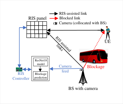
The contributions of this paper can be summarized as follows: We investigate the issue of blockage prediction for various locations of a mobile UE in the RIS-assisted wireless communication environment. We adopt the Doppler spread to capture the effect of the mobility of the UE on the channel characteristics. At first, the RGB camera is used to detect the presence of UE. This paper also considers deploying an RIS panel to differentiate between an absent or present but unblocked UE once the RGB camera cannot detect the unblocked UE. The unsuccessful detection of a UE, therefore, can be confirmed or mitigated using the RIS panel, as shown in Fig. 1. This allows detecting an absent, blocked, and unblocked UE at various locations using the RGB camera and RIS panel. We propose a deep learning-based framework to train the model to maximize the blockage probability prediction using an RGB camera at the BS and an RIS panel in the wireless channel. Note that we use the dataset from ViWi [12] to capture the RGB images from the BS. Detecting a blockage using the RGB camera, hence using the image, is a bit more difficult as the cases of absent UE and blocked UE are visually identical. This UE location detection is investigated as a ternary classification problem. Therefore, the RGB images and RIS panel-assisted-channel gains are coupled to detect the status of UE. In short, the proposed system model maximizes the probability of blockage prediction for various locations of UE with the help of the RIS panel and ViWi dataset.

The RIS passive elements reflect the incident signals towards the destination of interest. Each passive element is smaller than the wavelength. The elements adjust the reflection coefficient to re-experience the signals with nearly the same gain and proper beamforming into the directions of interest. The RIS panel elements properties are expressed by a diagonal matrix $\mathchar 29010\mathchar 8706\mathchar 29010$:

where $\mathchar 28939_{\mathchar 29033}\mathchar 12850\delimiter 67482370\mathchar 28720\mathchar 24891\mathchar 28721\delimiter 84267779$ defines amplitude reflection coefficient and $\mathchar 28946_{\mathchar 29033}$ is the passive element phase-shift, both for element $\mathchar 29033$.

These characteristics include the dependence on the environment geometry, frequency band, etc. As shown in Fig. 1, the UE receives the transmitted signals through the RIS panel. With the change of the UE locations, the blockage scenario changes. Hence, predicting the blockage is crucial due to the mobility of the UE to retain the system’s required quality of service. In wireless networks, many MPCs may be clustered into one or more spatial lobes, each represented by a mean angle of arrival (AoA). The authors in [14] reported that the received beam was contained within a single spatial lobe. Therefore, the proposed system model safely assumes that the received beam falls within one spatial lobe between two nodes while the other lobes have a trivial effect on the system. We assume the UE moves between $\mathchar 29013$ discrete locations while it travels, where $\mathchar 29045\mathchar 12349\mathchar 28721\mathchar 24891\mathchar 28722\mathchar 24891\mathchar 314\mathchar 314\mathchar 314\mathchar 24891\mathchar 29013$ and $\mathchar 29045$ is the index that refers to the current UE location. We define the number of MPCs as $\mathchar 29003\mathchar 12349\mathchar 29003^{\mathchar 29026}\mathchar 8235\mathchar 29003^{\mathchar 29042}\mathchar 8235\mathchar 29003^{\mathchar 29045}$, where $\mathchar 29003^{\mathchar 29026}$, $\mathchar 29003^{\mathchar 29042}$, and $\mathchar 29003^{\mathchar 29045}$ are the total number of resolvable MPCs during BS to UE location $\mathchar 29045$, BS to RIS, and RIS to UE location $\mathchar 29045$ links, respectively.

The rate between the BS and the UE location $\mathchar 29045$ through RIS panel is $\mathbf{\mathchar 29010_{\mathchar 29045}}\delimiter 67482370\mathchar 29035\delimiter 84267779\mathchar 12349\log\delimiter 67273472\mathbf{\mathchar 29001}\mathchar 8235\mathbf{\mathchar 29000_{\mathchar 29045}^{\mathchar 29039}}\delimiter 67482370\mathchar 29035\delimiter 84267779\delimiter 84054785$.

The RGB camera at the BS is equipped with complementary metal-oxide-semiconductor sensors and acquires colored images of UE and obstacles. The RGB camera computes the pixels based on their colors. The input image, $\mathchar 29016$ has the dimensions of $\mathchar 29000\mathchar 8706\mathchar 29015\mathchar 8706\mathchar 28995$, where $\mathchar 29000$, $\mathchar 29015$, and $\mathchar 28995$ define the height, width, and the number of colors of $\mathchar 29016$, respectively. Eventually, the RGB camera combines the color image captured directly through its filter with the other two colors captured by the pixels around it.

We determine the blocked and unblocked UE’s connections for location $\mathchar 29045$ with the help of RGB image and RIS panel to increase the reliability of wireless communications. We introduce an ordered pair $\delimiter 67273472\mathchar 29016\mathchar 24891\log\delimiter 67273472\mathbf{\mathchar 29001}\mathchar 8235\mathbf{\mathchar 29000_{\mathchar 29045}^{\mathchar 29039}}\delimiter 67482370\mathchar 29035\delimiter 84267779\delimiter 84054785\delimiter 84054785$, where the RGB images is $\mathchar 29016$ and the UE data RIS panel assisted rate is $\log\delimiter 67273472\mathbf{\mathchar 29001}\mathchar 8235\mathbf{\mathchar 29000_{\mathchar 29045}^{\mathchar 29039}}\delimiter 67482370\mathchar 29035\delimiter 84267779\delimiter 84054785$. The link status of UE at location $\mathchar 29045$ is expressed as $\mathchar 29036_{\mathchar 29045}\mathchar 12850\{\mathchar 8704\mathchar 28721\mathchar 24891\mathchar 28720\mathchar 24891\mathchar 28721\}$, where $\mathchar 8704\mathchar 28721$ defines the absent UE, $\mathchar 28720$ is present and unblocked UE, and $\mathchar 28721$ defines present but blocked UE. Maximizing the probability of blockage prediction over a number of UE locations $\mathchar 29013$ is:

where $\mathchar 29045\mathchar 12349\mathchar 28721\mathchar 24891\mathchar 28722\mathchar 24891\mathchar 314\mathchar 314\mathchar 314\mathchar 24891\mathchar 29013$ is the various locations of the mobile UE. The blockage prediction quantifies the degree of blockage incurs during the mobility for $\mathchar 29013$ locations. We, therefore, maximize the probability of predicted blockage using $\delimiter 67273472\mathchar 29016\mathchar 24891\log\delimiter 67273472\mathbf{\mathchar 29001}\mathchar 8235\mathbf{\mathchar 29000_{\mathchar 29045}^{\mathchar 29039}}\delimiter 67482370\mathchar 29035\delimiter 84267779\delimiter 84054785\delimiter 84054785$. Note that in (9), the product of the UE link status at location $\mathchar 29045$ is conditionally independent. $\mathchar 29009_{\mathchar 28672}\left\delimiter 67273472\mathchar 29016\mathchar 24891\log\delimiter 67273472\mathbf{\mathchar 29001}\mathchar 8235\mathbf{\mathchar 29000_{\mathchar 29045}^{\mathchar 29039}}\delimiter 67482370\mathchar 29035\delimiter 84267779\delimiter 84054785\right\delimiter 84054785$ is expressed as a prediction function and parameterized by a set of parameters $\mathchar 28672$. The output of the prediction function is a probability distribution function, $\cal\mathchar 28994$, of the UE locations over $\mathchar 29013$, where $\cal\mathchar 28994$ $\mathchar 12349\{\mathchar 29026_{\mathchar 28721}\mathchar 24891\mathchar 29026_{\mathchar 28722}\mathchar 24891\mathchar 314\mathchar 314\mathchar 314\mathchar 24891\mathchar 29026_{\mathchar 29013}\}$. We define the prediction function as follows:

Definition Recall that $\mathchar 29009_{\mathchar 28672}\delimiter 67273472\mathchar 29016\mathchar 24891\log\delimiter 67273472\mathbf{\mathchar 29001}\mathchar 8235\mathbf{\mathchar 29000_{\mathchar 29045}^{\mathchar 29039}}\delimiter 67482370\mathchar 29035\delimiter 84267779\delimiter 84054785\delimiter 84054785$ function is parameterized by a set $\mathchar 28672$ representing the parameters at the input. Let $\mathchar 29004\mathchar 12349\delimiter 67273472\mathchar 29016\mathchar 24891\log\delimiter 67273472\mathbf{\mathchar 29001}\mathchar 8235\mathbf{\mathchar 29000_{\mathchar 29045}^{\mathchar 29039}}\delimiter 67482370\mathchar 29035\delimiter 84267779\delimiter 84054785\delimiter 84054785$, and $\mathbb{\mathchar 29008}\delimiter 67273472\mathchar 29004\mathchar 24891\mathchar 29036\delimiter 84054785$ represents a joint probability distribution governing the relation between the observed sequence of RGB images and RIS-assisted link to detect the blockage, $\mathchar 29004$. Whether blocked or not, the future location-independent link status is defined as $\mathchar 29036$, reflecting the probabilistic nature of link blockages for a $\mathchar 29013$ number of UE locations. An independent location $\mathchar 29045$ of $\mathbb{\mathchar 29008}\delimiter 67273472\mathchar 29004_{\mathchar 29045}\mathchar 24891\mathchar 29036_{\mathchar 29045}\delimiter 84054785$ is sampled from $\mathbb{\mathchar 29008}\delimiter 67273472\mathchar 29004\mathchar 24891\mathchar 29036\delimiter 84054785$ serves as a label for the observed $\mathchar 29004_{\mathchar 29045}$. This sampling helps maximizing the prediction function $\mathchar 29009_{\mathchar 28672}\delimiter 67273472\mathchar 29016\mathchar 24891\log\delimiter 67273472\mathbf{\mathchar 29001}\mathchar 8235\mathbf{\mathchar 29000_{\mathchar 29045}^{\mathchar 29039}}\delimiter 67482370\mathchar 29035\delimiter 84267779\delimiter 84054785\delimiter 84054785$ to maintain high-fidelity predictions.

The blockage probability index, $\mathchar 29033$, of the UE locations over $\mathchar 29013$ are also independent. We express $\mathchar 29033$ in the following formulation as follows:

where $\mathchar 29026_{\mathchar 29033}$ defines the blockage probability for the UE location $\mathchar 29033$. Neural network model maximizes the prediction function, $\mathchar 29009_{\mathchar 28672}\left\delimiter 67273472\mathchar 29016\mathchar 24891\log\delimiter 67273472\mathbf{\mathchar 29001}\mathchar 8235\mathbf{\mathchar 29000_{\mathchar 29045}^{\mathchar 29039}}\delimiter 67482370\mathchar 29035\delimiter 84267779\delimiter 84054785\right\delimiter 84054785$, and then predicts the probability of the blockage for UE location $\mathchar 29045$, using $\mathchar 29009_{\mathchar 28672}\left\delimiter 67273472\mathchar 29016\mathchar 24891\log\delimiter 67273472\mathbf{\mathchar 29001}\mathchar 8235\mathbf{\mathchar 29000_{\mathchar 29045}^{\mathchar 29039}}\delimiter 67482370\mathchar 29035\delimiter 84267779\delimiter 84054785\right\delimiter 84054785$ (details are provided in Section III-B). $\mathchar 29009_{\mathchar 28672}\left\delimiter 67273472\mathchar 29016\mathchar 24891\log\delimiter 67273472\mathbf{\mathchar 29001}\mathchar 8235\mathbf{\mathchar 29000_{\mathchar 29045}^{\mathchar 29039}}\delimiter 67482370\mathchar 29035\delimiter 84267779\delimiter 84054785\right\delimiter 84054785$ is, therefore, computed in a way to find the probability mass function of $\mathchar 29013$, hence, maximizing the probability of blockage prediction. In other words, while the objective function maximizes the probability of blockage prediction, the model finds the optimal prediction function for a given RGB image and RIS panel-assisted link, as well as $\mathchar 28672$. The image of the RGB camera and RIS-assisted link are fed to the neural network model to determine the status of the UE at $\mathchar 29045$ location. We have three outcomes to determine the link status of UE location $\mathchar 29045$, (1) UE is present and unblocked, (2) UE is present but blocked, and (3) absent UE.

The neural network model fed with an RGB camera and RIS panel-based channel modeling is presented in Fig. 1. We adopt residual network (ResNet)-18 neural network model, where 1) the model aims to learn and maximize $\mathchar 29009_{\mathchar 28672}\delimiter 67273472\mathchar 29016\mathchar 24891\log\delimiter 67273472\mathbf{\mathchar 29001}\mathchar 8235\mathbf{\mathchar 29000_{\mathchar 29045}^{\mathchar 29039}}\delimiter 67482370\mathchar 29035\delimiter 84267779\delimiter 84054785\delimiter 84054785$, 2) the model maximizes (9) using optimal $\mathchar 29009_{\mathchar 28672}\delimiter 67273472\mathchar 29016\mathchar 24891\log\delimiter 67273472\mathbf{\mathchar 29001}\mathchar 8235\mathbf{\mathchar 29000_{\mathchar 29045}^{\mathchar 29039}}\delimiter 67482370\mathchar 29035\delimiter 84267779\delimiter 84054785\delimiter 84054785$. We train the model, ensuring it fits the blockage prediction model. Note that $\mathchar 28672$, and $\delimiter 67273472\mathchar 29016\mathchar 24891\log\delimiter 67273472\mathbf{\mathchar 29001}\mathchar 8235\mathbf{\mathchar 29000_{\mathchar 29045}^{\mathchar 29039}}\delimiter 67482370\mathchar 29035\delimiter 84267779\delimiter 84054785\delimiter 84054785$ serve as the input of the neural network model. This model is trained, followed by supervised learning, using the RGB image and RIS panel-assisted channel modeling from the environment labeling with their corresponding blockage index. At least two neuron layers are fully connected in the model. The adopted model is based on deep convolution neural networks, transferable learning, and predictive learning function. Additionally, its final fully connected layer is removed and replaced with another fully connected layer with several neurons equal to the number of UE locations over $\mathchar 29013$. Additionally, $\mathchar 29009_{\mathchar 28672}\delimiter 67273472\mathchar 29016\mathchar 24891\log\delimiter 67273472\mathbf{\mathchar 29001}\mathchar 8235\mathbf{\mathchar 29000_{\mathchar 29045}^{\mathchar 29039}}\delimiter 67482370\mathchar 29035\delimiter 84267779\delimiter 84054785\delimiter 84054785$ maps the RGB image and relates to a blockage probability, $\mathchar 29026_{\mathchar 29033}$. During the training process, a cross-entropy loss is $\mathchar 29039\mathchar 12349\mathchar 4944\displaylimits_{\mathchar 29034\mathchar 12349\mathchar 28721}^{\mathchar 29013}\mathchar 29036_{\mathchar 29034}\log\mathchar 29026_{\mathchar 29034}$, where $\mathchar 29026_{\mathchar 29034}$ is the probability mass function, which is induced by the soft-max layer. The model also aims to find minimal cross-entropy loss The relation between the cross-entropy loss nature and the UE location $\mathchar 29045$ is inversely proportional, i.e., lower entropy loss results in finding the UE location $\mathchar 29045$ tends to be deterministic than the random nature. The detection of the UE at location $\mathchar 29045$ is treated as a ternary classification problem, such as blocked, unblocked, or absent UE at location $\mathchar 29045$. The authors in [13] demonstrated that neural networks effectively learned to block prediction probability. The network is, therefore, trained to detect the UE at location $\mathchar 29045$, by using the blockage index, achieved from $\mathchar 29009_{\mathchar 28672}\delimiter 67273472\mathchar 29016\mathchar 24891\log\delimiter 67273472\mathbf{\mathchar 29001}\mathchar 8235\mathbf{\mathchar 29000_{\mathchar 29045}^{\mathchar 29039}}\delimiter 67482370\mathchar 29035\delimiter 84267779\delimiter 84054785\delimiter 84054785$. At first, using $\mathchar 29016$, the neural network model resolves of the UE is present and unblocked at location $\mathchar 29045$. If the detection at location $\mathchar 29045$ is not successful, $\log\delimiter 67273472\mathbf{\mathchar 29001}\mathchar 8235\mathbf{\mathchar 29000_{\mathchar 29045}^{\mathchar 29039}}\delimiter 67482370\mathchar 29035\delimiter 84267779\delimiter 84054785\delimiter 84054785$ detects the blockage scenarios, including present but blocked, and absent UE at location $\mathchar 29045$. This approach labels RIS panel-assisted link and image, $\mathchar 29016$, and then uses them for the training model and is performed with ImageNet data [16]. Using a deep neural network, blockage prediction involves detecting UE locations over a $\mathchar 29013$, followed by RIS-assisted link assessment. The detection of UE location $\mathchar 29045$, therefore, maximizing the probability of blockage detection, is summarized in Algorithm 1.

Algorithm 1 maximizes the probability of the blockage prediction. $\cal\mathchar 28994$ is produced in various UE locations $\mathchar 29013$. Using the RIS panel, $\mathbf{\mathchar 29000_{\mathchar 29045}^{\mathchar 29039}}\delimiter 67482370\mathchar 29035\delimiter 84267779$ is calculated. Then ResNet-18 model plays a role in finding the existence of UE location $\mathchar 29045$ using the dataset and results in the link status as $\mathchar 29036_{\mathchar 29045}\mathchar 12349\mathchar 28721$. For an unsuccessful detection UE at the location, $\mathchar 29045$, the RIS-assisted channel gain helps to detect whether $\mathchar 29036_{\mathchar 29045}$ is -1 or 0 or 1.

References

• [1] C. Huang et al., ”Holographic MIMO surfaces for 6G wireless networks: Opportunities, challenges, and trends,” IEEE Wireless Communications, vol. 27, no. 5, pp. 118-125, 2020
• [2] G. Yang, X. Xu, and Y. Liang, ”Intelligent reflecting surface assisted non-orthogonal multiple access,” 2019, arXiv:1907.03133. [Online]. Available: http://arxiv.org/abs/1907.03133
• [3] E. Bjornson, O. OZdogan, and E. Larsson, ”Intelligent reflecting surface versus decode-and-forward: How large surfaces are needed to beat relaying?,” IEEE Wireless Communications Letters, vol. 9, no. 2, pp. 244-248, Feb. 2020
• [4] M. Alrabeiah and A. Alkhateeb, ”Deep learning for TDD and FDD massive MIMO: mapping channels in space and frequency,” 53rd Asilomar Conference on Signals, Systems, and Computers, 2019, pp. 1465-1470
• [5] C. Huang, A. Zappone, G. C. Alexander, M. Debbah, and C. Yuen, ”Large Intelligent Surfaces for Energy Efficiency in Wireless Communication,” arXiv:1810.06934, Oct 2018
• [6] S. V. Hum and J. Perruisseau-Carrier, ”Reconfigurable reflectarrays and array lenses for dynamic antenna beam control: A review,” IEEE Transactions on Antennas and Propagation, vol. 62, no. 1, pp. 183–198, Jan 2014
• [7] C. Liaskos, S. Nie, A. Tsioliaridou, A. Pitsillides, S. Ioannidis, and I. Akyildiz, ”A new wireless communication paradigm through software-controlled metasurfaces,” IEEE Communications Magazine, vol. 56, no. 9, pp. 162–169, Sep. 2018
• [8] L. Sanguinetti, E. Bjornson, and J. Hoydis, ”Towards Massive MIMO 2.0: Understanding spatial correlation, interference, suppression, and pilot contamination,” arXiv e-prints, p. arXiv:1904.03406, Apr 2019
• [9] X. Li and A. Alkhateeb, ”Deep learning for direct hybrid precoding in millimeter-wave massive MIMO systems,” in Proc. of Asilomar s, arXiv e-prints, p. arXiv:1905.13212, May 2019
• [10] F. B. Mismar and B. L. Evans, ”Partially blind handovers for mmwave new radio aided by sub-6 GHz LTE signaling,” in Pro 2018 IEEE International Conference on Communications Workshops, pp. 1–5
• [11] M. Eisen, C. Zhang, L. F. O. Chamon, D. D. Lee, and A. Ribeiro, ”Learning optimal resource allocations in wireless systems,” IEEE Transactions on Signal Processing, vol. 67, no. 10, pp. 2775–2790, May 2019
• [12] https://www.viwi-dataset.net/
• [13] M. Alrabeiah and A. Alkhateeb, ”Deep learning for mmwave beam and blockage prediction using sub-6 GHz channels,” IEEE Transactions on Communications, vol. 68, no. 9, pp. 5504–5518, 2020
• [14] M. Samimi and T. Rappaport, ”3-D millimeter-wave statistical channel model for 5G wireless system design,” IEEE Transactions on Microwave Theory and Techniques, vol. 64, no. 7, pp. 2207-2225, July 2016
• [15] B. Akgun, M. Krunz, and D. Manzi, ”Impact of Beamforming on Delay Spread in Wideband Millimeter-wave Systems,” International Conference on Computing, Networking, and Communications, 2020, pp. 890-896
• [16] O. Russakovsky, J. Deng, H. Su, J. Krause, S. Satheesh, S. Ma, Z. Huang, A. Karpathy, A. Khosla, M. Bernstein et. al., ”Imagenet large scale visual recognition challenge,” International journal of computer vision, vol. 115, no. 3, pp. 211–252, 2015