Investigating shock wave propagation, evolution, and anisotropy using a moving window concurrent atomistic-continuum framework

We consider a two-dimensional monatomic lattice with no defects under compression by an ideal longitudinal shock wave traveling in the $x-$direction. Mathematically, we represent the shock as a propagating discontinuity across which there exists a jump in particle velocity ($v$), stress ($\sigma$), strain ($\epsilon$), and temperature ($\theta$). Material quantities ahead of the shock front have the superscript $-$, and quantities behind the shock front have the superscript $+$. The notation $\llbracket\cdot\rrbracket$ denotes the change in a given quantity $(\cdot)$ across the shock front. During each simulation, particles ahead of the shock wave are assumed to be at zero mean particle velocity, unstressed, unstrained, and at room temperature ($295$ K). Furthermore, the shock propagates at a natural velocity $U_{S}$ along the surface of the primitive unit cell of an FCC lattice. We incorporate these parameters into a moving window CAC framework to simulate long-time shock wave propagation over engineering-scale domains. Specifically, we model the classic Riemann problem of a single shock wave front with constant states on either side as shown in Fig. 1.

To calculate the aforementioned jump parameters and thus characterize the shock wave at the continuum level, we use two different formulations which are discussed below.

First, we simulate dynamic shock wave propagation and evolution using the conservation of momentum, continuity equation, Hugoniot equation of state (EOS), and a thermodynamic relationship derived from the shock Hugoniot and release isentrope. By applying the conservation of linear momentum and continuity of displacement across the discontinuous shock front and assuming uniaxial loading, we obtain the following standard one-dimensional shock wave jump equations davison2008fundamentals:

	$\displaystyle\llbracket\sigma\rrbracket+\rho U_{s}\llbracket v\rrbracket$	$\displaystyle=0$		(1)
	$\displaystyle\llbracket v\rrbracket+U_{s}\llbracket\epsilon\rrbracket$	$\displaystyle=0$		(2)

where $\rho$ denotes the density of the material. To fully parameterize the system, Eqs. (1) and (2) are supplemented by an empirically observed linear relation between shock velocity and particle velocity meyers1994dynamic:

$$U_{s}=C_{0}+S\llbracket v\rrbracket.$$

(3)

Here, S is a dimensionless, empirical parameter representing the slope of the shock velocity vs. particle velocity Hugoniot curve, and $C_{0}$ is the sound velocity in the material at zero stress. We can use Eqs. (1), (2), and (3) to derive the standard Hugoniot stress-strain relationship given as follows:

$$\sigma=\frac{\rho C_{0}^{2}\llbracket\epsilon\rrbracket}{(1+S\llbracket\epsilon\rrbracket)^{2}}$$

(4)

where compressive stress and strain are considered positive. The Hugoniot stress-strain relationship forms the basis of modern equations of state. Finally, we calculate the rise in temperature across the shock front by solving the following ordinary differential equation davison2008fundamentals:

$$C_{V}\left(\frac{d\theta}{d\epsilon}\right)_{H}-\frac{\gamma\theta C_{V}}{1-\epsilon}=\frac{\epsilon}{2}\left(\frac{d\sigma}{d\epsilon}\right)_{H}-\frac{\sigma}{2}$$

(5)

where $C_{V}$ is the volumetric specific heat capacity, and $\gamma$ is the Mie-Gruneisen parameter for the material.

We also characterize the propagating shock wave using the nonlinear Eulerian thermoelastic shock equations derived in clayton2013nonlinear, clayton2014shock for anisotropic crystals. Nonlinear elastic constitutive models of material behavior which do not account for slippage and plasticity are generally idealizations because even small uniaxial compressive strains can cause ductile materials to reach the experimental Hugoniot elastic limit (HEL). However, such elastic formulations can be practically applied to defect-free atomistic and multiscale simulations since these domains may be shocked to finite strains over relatively short time scales and small volumes clayton2014shock, zimmerman2011elastic.

For an extensive derivation of the Eulerian formulation for shock waves, we refer the reader to clayton2013nonlinear. Here, we merely present the relevant equations used in the current work. The particle velocity in the shocked material, shock propagation velocity, and temperature in the shocked material are given by the following respective equations:

$$v=\biggl\{\left(\frac{\hat{S}}{\rho}\right)\left[\left(1-2D\right)-\left(1-2D\right)^{3/2}\right]\biggr\}^{1/2}$$

(6)

$$U_{S}=v\left[1-\left(1-2D\right)^{-1/2}\right]^{-1}$$

(7)

$$\theta=\frac{\partial\hat{U}}{\partial\eta}=\theta_{0}\left(1-\hat{\Gamma}_{1}D-\frac{1}{2}\hat{\Gamma}_{11}D^{2}\right).$$

(8)

In Eqs. (6), (7), and (8), $D$ is the Eulerian strain represented by the following expression:

$$D=\frac{1}{2}\left(1-F^{-2}\right)=\frac{1}{2}\left[1-\frac{1}{(1+\epsilon)^{2}}\right].$$

(9)

Here, the term Eulerian refers to a strain which is a function of the inverse deformation gradient $F$. Hence, the strain tensor $D$ assumes material coordinates rather than spatial coordinates, so it can be applied to simulations of anisotropic materials clayton2013nonlinear. Furthermore, $\hat{U}$ is the Eulerian fourth-order internal energy function as seen below clayton2014shock:

$$\hat{U}=\frac{1}{2}\hat{C}_{11}D^{2}+\frac{1}{6}\hat{C}_{111}D^{3}+\frac{1}{24}\hat{C}_{1111}D^{4}-\theta_{0}\left(\hat{\Gamma}_{1}D+\frac{1}{2}\hat{\Gamma}_{11}D^{2}-1\right)\eta$$

(10)

where $\hat{C}_{11}$, $\hat{C}_{111}$, and $\hat{C}_{1111}$ are the Eulerian second, third, and fourth-order elastic constants, $\hat{\Gamma}_{1}$ and $\hat{\Gamma}_{11}$ are the Eulerian first and second-order Grüneisen parameters, and $\eta=0$ is the entropy ahead of the shock front. The elastic constants and Grüneisen parameters in an Eulerian setting are obtained from their non-Eulerian counterparts using the following relations weaver1976application, perrin1978application, clayton2013nonlinear:

	$\displaystyle\hat{C}_{11}$	$\displaystyle=C_{11}$		(11)
	$\displaystyle\hat{C}_{111}$	$\displaystyle=C_{111}+12C_{11}$		(12)
	$\displaystyle\hat{C}_{1111}$	$\displaystyle=C_{1111}-18C_{111}-318C_{11}$		(13)
	$\displaystyle\hat{\Gamma}_{1}$	$\displaystyle=\Gamma_{1}$		(14)
	$\displaystyle\hat{\Gamma}_{11}$	$\displaystyle=\Gamma_{11}+4\Gamma_{1}.$		(15)

Finally, the conjugate stress $\hat{S}$ is represented by

	$\displaystyle\hat{S}$	$\displaystyle=\frac{\partial\hat{U}}{\partial D}$		(16)
		$\displaystyle=C_{11}D+\frac{1}{2}\hat{C}_{111}D^{2}+\left(\frac{1}{6}\hat{C}_{1111}-\theta_{0}\hat{\Gamma}_{1}b_{3}\right)D^{3}-\theta_{0}D^{4}\left[\left(\hat{\Gamma}_{1}b_{4}+\hat{\Gamma}_{11}b_{3}\right)+\left(\hat{\Gamma}_{1}b_{5}+\hat{\Gamma}_{11}b_{4}\right)D\right]$

where $b_{3}$, $b_{4}$, and $b_{5}$ are polynomials for entropy $\eta$ generated across the shock front, and their expressions can be found in clayton2013nonlinear. In each shock wave simulation, we use the fourth-order expression of Eqs. (6), (7), and (8).

To legitimately utilize the shock equations from Sec. 2.3 as well as avoid intractability with the moving window techniques, we perform shock simulations with relatively small strains such that the resulting stresses are below the HEL of the material (see A.2). To maintain consistency, we refer to these as elastic shock waves in the present work, but they are also classified as weak shocks in other papers holian1995atomistic. Elastic shock waves are often modeled in defect-free crystals with NEMD techniques to study a particular phenomenon, test a new framework, or validate a given potential holian1978molecular, zimmerman2011elastic, davis2020one, and their distinguishing characteristic is the lack of any permanent dislocations (inelastic deformation) behind the wave front. This is possible because the HEL is typically higher than what is seen in experimental settings yang2013concurrent, and the wave speed is still greater than the sound velocity in the material at the low strains. Modeling shock propagation with the CAC moving window framework using thermoelastic-viscoplastic models lloyd2014simulation, lloyd2014plane is a worthy pursuit but would add an extra layer of complexity to the current model and is thus reserved for future studies.

The two-dimensional CAC framework is implemented using an in-house C++ code, and the monatomic lattice is split into three primary regions as seen in Fig. 2. The two coarse-scaled (continuum) regions are composed of rhombus elements, and the four particles which make up any particular element are referred to as nodes in the present work. We choose rhombus elements because they align with the primitive unit cell of the FCC lattice (see Sec. 4.2) and thus facilitate a smooth transition between the fine-scaled and coarse-scaled regions. Specifically, the $x$-direction corresponds to the [112] lattice orientation while the $y$-direction corresponds to the [110] lattice orientation. Since element connectivity is not required in CAC xiong2011coarse, each node is a member of only one element, and this greatly reduces the complexity of the finite element formulation. Furthermore, the edges of the grid in the continuum regions are “filled in" with particles which we refer to as boundary atoms in this work. This is done in order to facilitate periodic boundary conditions as shown in xu2015quasistatic.

The two coarse-scaled regions flank the inner fine-scaled (atomistic) region on the left and right-hand side, and we refer to the particles in this region as either inner atoms or just atoms in the present work. The “elements" in the fine-scaled region are reduced to their smallest possible configuration such that only four atoms constitute the entire area of each element. Hence, both the fine-scaled and coarse-scaled regions are technically made up of rhombuses with the only differences being the area and mass of their respective elements. As a consequence, one governing equation along with a single mass matrix is utilized for both regions, all force calculations are nonlocal, and the interatomic potential is the only constitutive relation xu2016mesh. Thus, the particles at the A-C interfaces ($x_{A,0}$ and $x_{A,F}$) interact with each other directly without creating ghost forces xu2015quasistatic, xu2018pycac.

We note that to avoid introducing non-physical strains into the domain during shock simulations, semi-periodic boundary conditions are employed in the $x$-direction whereby the particles at the ends of the chain ($x_{0}$ and $x_{F}$) are made neighbors with the nodes at the interfaces ($x_{A,0}$ and $x_{A,F}$ respectively) davis2022moving. Additionally, since the present work only considers uniaxial compression, we utilize periodic boundary conditions in the $y$-direction when modeling a longitudinal shock wave.

To calculate the integrand of the internal force density (Eq. 20), we use the modified Morse interatomic potential function. This potential only considers first nearest neighbor interactions and is given by the following expression macdonald1981thermodynamic:

$$\Pi(r_{ij})=\frac{D_{0}}{2B-1}\left[\mathrm{e}^{-2\alpha\sqrt{B}(r_{ij}-r_{0})}-2B\mathrm{e}^{-\alpha(r_{ij}-r_{0})/\sqrt{B}}\right]$$

(17)

where $r_{ij}=|\textbf{x}_{i}-\textbf{x}_{j}|$ is the magnitude of the displacement between particle $i$ and $j$, and $r_{0}$ is the distance at which the potential reaches the minimum (defined as the close-packed neighbor spacing). We perform shock simulations with Cu and Al, and the parameters for these materials are given in Table 1.

The CAC governing equation (Eq. 24) is a second-order ordinary differential equation in time, and we solve it using the velocity Verlet algorithm. The time step used in the integration algorithm is chosen to be $\Delta t=0.001$ ps in order to minimize numerical error.

To apply temperature to the domain, we use the Langevin thermostat – a stochastic thermostat which adds a random force to the particle motion along with a damping term $\zeta$. In particular, we modify the velocity Verlet algorithm in the presence of the Langevin thermostat by performing the discretization used in LAMMPS schneider1978molecular:

	$\displaystyle\textbf{v}_{i}\left(t+\frac{\Delta t}{2}\right)$	$\displaystyle=\textbf{v}_{i}(t)-\frac{\Delta t}{2}\left[\frac{\nabla_{i}\Pi(t)}{m}+\zeta\textbf{v}_{i}(t)\right]+\sqrt{\frac{\Delta tk_{B}\theta\zeta}{m}}\tilde{\textbf{h}}_{i}$
	$\displaystyle\textbf{x}_{i}(t+\Delta t)$	$\displaystyle=\textbf{x}_{i}(t)+\textbf{v}_{i}\left(t+\frac{\Delta t}{2}\right)\Delta t$
	$\displaystyle\textbf{v}_{i}\left(t+\Delta t\right)$	$\displaystyle=\textbf{v}_{i}\left(t+\frac{\Delta t}{2}\right)-\frac{\Delta t}{2}\left[\frac{\nabla_{i}\Pi(t+\Delta t)}{m}+\zeta\textbf{v}_{i}\left(t+\frac{\Delta t}{2}\right)\right]+\sqrt{\frac{\Delta tk_{B}\theta\zeta}{m}}\tilde{\textbf{h}}_{i}.$		(18)

Here, $\textbf{x}_{i}$ and $\textbf{v}_{i}$ denote the position and velocity of the ${i}^{th}$ particle, $m$ is the atomic mass, $k_{B}$ is Boltzmann’s constant, and $\tilde{\textbf{h}}_{i}$ is a Gaussian random variable with a mean of zero and a variance of one. As per Langevin’s requirements, we generate a different random variable for each particle during each velocity update. Since Langevin is local in nature, the target temperatures $\theta^{+}$ and $\theta^{-}$ are specified for each particle. For the compressive strains applied in this work, $\theta^{+}$ has an upper boundary of $\sim$ 450 K.

In Table 2, we present the empirical Hugoniot shock parameters as well as the second, third, and fourth-order elastic constants (in a normal and Eulerian setting) for both Cu and Al. The Hugoniot parameters are obtained from marsh1980lasl, the second and third-order elastic constants for Cu and Al are obtained from hiki1966anharmonicity and thomas1968third respectively, and the fourth-order elastic constants are obtained from clayton2014shock. For these values, the temperature is assumed to be $295$ K, $C_{0}$ is given in $km/sec$, $S$ is unitless, and the elastic constants are given in GPa. The Hugoniot parameters are derived for a shock wave propagating through a bulk, polycrystalline material. Furthermore, the elastic constants represent the pure-mode directions such that a planar shock impact results in an exclusively longitudinal component (along the [100] direction) with no transmitted shear stress, and hence the one-dimensional analysis is valid. We use these parameters as initial input in our shock simulations and compare the results from the CAC model to analytical and empirical data in Sec. 6.

Here, we give a very brief overview of the finite element implementation of CAC, but more details can be found in xiong2009multiscale, deng2010coarse, xiong2011coarse, chen2019concurrent. The mathematical foundation of CAC is Atomistic Field Theory (AFT), and the governing equations of AFT have a similar form to the balance laws of classical continuum mechanics. Exploiting the definitions of internal force density and kinetic temperature derived in chen2005nanoscale and chen2006local, we can recast the instantaneous balance equation of linear momentum as follows xiong2009multiscale:

$$\rho^{\alpha}\ddot{\textbf{u}}^{\alpha}(\textbf{x})=\textbf{f}_{int}^{\alpha}(\textbf{x})+\textbf{f}^{\alpha}(\textbf{x}).$$

(19)

In Eq. (19), $\textbf{u}^{\alpha}(\textbf{x})$ is the displacement of the $\alpha^{th}$ atom in the unit cell, $\rho^{\alpha}=m^{\alpha}/\Delta V$ is the volumetric mass density, $m^{\alpha}$ is the mass of the $\alpha^{th}$ atom, $\Delta V$ is the volume of the unit cell, $\textbf{f}_{int}^{\alpha}(\textbf{x})$ is the internal force density, and $\textbf{f}^{\alpha}(\textbf{x})$ is the force density due to external forces and temperature. The two terms on right side of Eq. (19) are represented as follows:

	$\displaystyle\textbf{f}_{int}^{\alpha}(\textbf{x})$	$\displaystyle=\int_{\Omega(\textbf{x}^{\prime})}\sum_{\beta=1}^{N_{a}}\textbf{f}\left[\textbf{u}^{\alpha}(\textbf{x})-\textbf{u}^{\beta}(\textbf{x}^{\prime})\right]d\textbf{x}^{\prime}$		(20)
	$\displaystyle\textbf{f}^{\alpha}(\textbf{x})$	$\displaystyle=\textbf{f}_{ext}^{\alpha}(\textbf{x})-\frac{m^{\alpha}k_{B}}{M\Delta V}\nabla_{\textbf{x}}\theta^{\alpha}$		(21)

where $\textbf{f}_{ext}^{\alpha}(\textbf{x})$ is the external force density, $M$ is the total mass of the atoms within a unit cell, and $\theta^{\alpha}$ is the kinetic temperature. We note that the internal force density can be obtained exclusively from the interatomic potential function since it is a nonlinear, nonlocal function of relative displacements between neighboring particles yang2014concurrent.

We employ the finite element method to calculate the numerical solution of Eq. (19). We populate the domain with finite elements such that every element contains a collection of primitive unit cells. Each nodal location represents a unit cell which is itself made up of particles. As a result, CAC provides a two-level description of crystals and follows the solid state physics model whereby the structure is continuous at the lattice level but discrete at the atomic scale. We use interpolation within each element in the domain to approximate the displacement field as follows xiong2011coarse:

$$\hat{\textbf{u}}^{\alpha}(\textbf{x})=\bm{\Phi}_{\xi}(\textbf{x})\textbf{U}_{\xi}^{\alpha}.$$

(22)

In Eq. (22), $\hat{\textbf{u}}^{\alpha}(\textbf{x})$ is the displacement field for the $\alpha^{th}$ atom within a given element, $\bm{\Phi}_{\xi}(\textbf{x})$ is the shape function, and $\textbf{U}_{\xi}^{\alpha}$ is the displacement of the $\alpha^{th}$ atom within the $\xi^{th}$ element node. We let $\xi=1,2,...,n$ where $n$ is the total number of nodes in the element (four in this work).

Applying the method of weighted residuals, we obtain the weak form of the governing equation by multiplying Eq. (19) with a weight function $\bm{\Phi}_{\eta}(\textbf{x})$ and integrating over the entire domain:

$$\int_{\Omega(\textbf{x})}\left[\rho^{\alpha}\bm{\Phi}_{\eta}(\textbf{x})\ddot{\textbf{u}}^{\alpha}(\textbf{x})\right]d\textbf{x}=\int_{\Omega(\textbf{x})}\left[\bm{\Phi}_{\eta}(\textbf{x})\textbf{f}_{int}^{\alpha}(\textbf{x})\right]d\textbf{x}+\int_{\Omega(\textbf{x})}\left[\bm{\Phi}_{\eta}(\textbf{x})\textbf{f}^{\alpha}(\textbf{x})\right]d\textbf{x}.$$

(23)

Specifically, the Galerkin method is used to obtain the above expression, so the weight function $\bm{\Phi}_{\eta}(\textbf{x})$ equals the shape function $\bm{\Phi}_{\xi}(\textbf{x})$ in this case. Substituting Eqs. (20), (21), and (22) into Eq. (23), we arrive at the weak form of the CAC governing equation which can be represented in matrix form as follow:

$$\textbf{M}^{\alpha}\ddot{\textbf{U}}_{\xi}^{\alpha}=\textbf{F}_{int}^{\alpha}+\textbf{F}^{\alpha}$$

(24)

where

	$\displaystyle\textbf{M}^{\alpha}$	$\displaystyle=\int_{\Omega(\textbf{x})}\left[\rho^{\alpha}\bm{\Phi}_{\eta}(\textbf{x})\bm{\Phi}_{\xi}(\textbf{x})\right]d\textbf{x}$		(25)
	$\displaystyle\textbf{F}_{int}^{\alpha}$	$\displaystyle=\int_{\Omega(\textbf{x})}\bm{\Phi}_{\eta}(\textbf{x})\int_{\Omega(\textbf{x}^{\prime})}\sum_{\beta=1}^{N_{a}}\textbf{f}\left[\bm{\Phi}_{\xi}(\textbf{x})\textbf{U}_{\xi}^{\alpha}-\bm{\Phi}_{\xi}(\textbf{x}^{\prime})\textbf{U}_{\xi}^{\beta}\right]d\textbf{x}^{\prime}d\textbf{x}$		(26)
	$\displaystyle\textbf{F}^{\alpha}$	$\displaystyle=\int_{\Omega(\textbf{x})}\left[\bm{\Phi}_{\eta}(\textbf{x})\textbf{f}^{\alpha}(\textbf{x})\right]d\textbf{x}.$		(27)

In this work, we approximate the inertial term (Eq. 25) using the lumped mass matrix derived in B.1. Additionally, no external forces are applied, and temperature is incorporated via a thermostat as in xiong2014prediction and chen2018passing. The internal force density $\textbf{F}_{int}^{\alpha}$ is the most computationally expensive term, and we evaluate it numerically using Gaussian integration as discussed in B.2.

By using this finite element implementation of CAC, a majority of the degrees of freedom in the coarse-scaled regions are eliminated. For critical regions where atomistic behavior is required, the finest mesh is used such that each rhombus “element" consists exclusively of four atoms with no additional lattice points. Thus, CAC uses AFT to produce a unified theoretical framework between the fine-scaled and coarse-scaled regions. A unique feature of CAC is that in the finite element implementation, element connectivity is not required because the nonlocal interatomic force field is the only constitutive relation xiong2011coarse. This is similar to aspects of the cohesive zone model needleman1987continuum and greatly simplifies the implementation of both the mass matrix as well as the force calculations.

Rhombohedral elements are utilized within the CAC formulation to replicate the primitive unit cell of a monocrystalline lattice (FCC in the present work). A sketch of this can be seen in Fig. 3(a), where we observe the primitive unit cell (blue lines) within the broader FCC crystal structure.

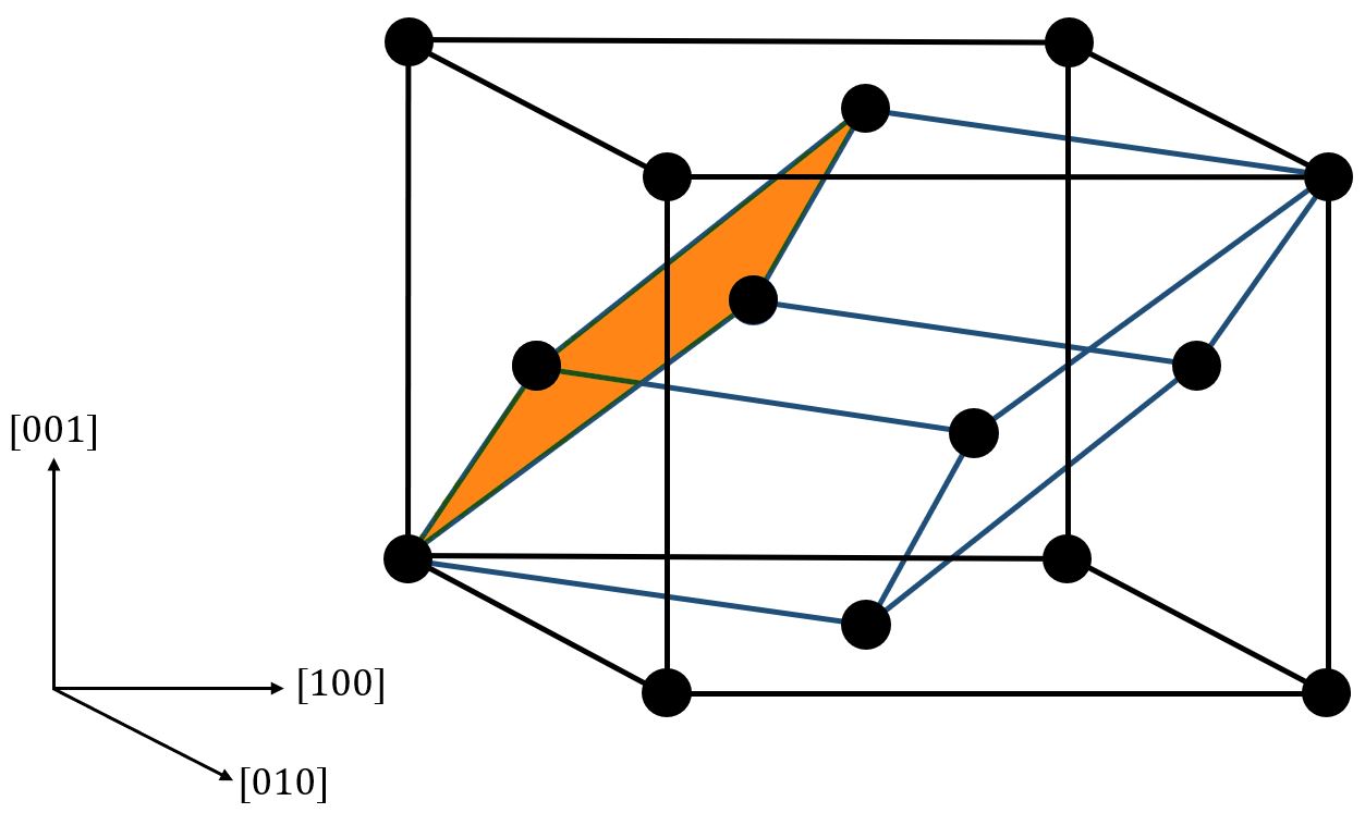
Furthermore, the shaded region represents the two-dimensional atomic plane used in our formulation whereby rhombus elements are incorporated throughout the domain. Since the same constitutive relation is used both within elements as well as between elements, dislocations and cracks emerge naturally through the separation of finite elements xiong2011coarse. This is a direct result of the CAC governing equations, and it allows such defects to pass smoothly between the atomistic and continuum regions without deforming individual elements.

A schematic of the two-dimensional rhombus element can be seen in Fig. 3(b). Here, the black circles represent the four nodes where the governing equations are applied, and the grey circles represent the lattice points which serve as nodal neighbors and thus aid in the force calculations. For monatomic crystals, each nodal location (unit cell) only contains one atom, and the positions of the lattice points are interpolated using Eq. (22) throughout the element. We emphasize that the lattice points are excluded from the Verlet algorithm. Finally, since no external forces are applied in this work, the governing equations from Sec. 4.1 reduce to the following:

$$\textbf{M}\ddot{\textbf{U}}-\textbf{F}^{int}=\textbf{0}$$

(28)

where

$$\textbf{M}=\int_{\Omega(\textbf{x})}\left[\rho\bm{\Phi}(\textbf{x})\bm{\Phi}(\textbf{x})\right]d\textbf{x}$$

(29)

$$\textbf{F}^{int}=\int_{\Omega(\textbf{x})}\bm{\Phi}(\textbf{x})\int_{\Omega(\textbf{x}^{\prime})}\sum_{j=1}^{n_{\alpha}}\textbf{f}\left[\bm{\Phi}(\textbf{x})\textbf{U}_{i}-\bm{\Phi}(\textbf{x}^{\prime})\textbf{U}_{j}\right]d\textbf{x}^{\prime}d\textbf{x}=\int_{\Omega(\textbf{x})}\bm{\Phi}(\textbf{x})\textbf{f}^{int}(\textbf{x})d\textbf{x}.$$

(30)

In Eq. (28), M is the mass matrix, and B.1 provides a full derivation of this term. In brief, we utilize the lumped mass matrix approach in the present formulation which effectively reduces M to the following expression for each element:

$$\textbf{M}=\frac{mN_{ppe}}{N_{npe}}$$

(31)

where $m$ is the atomic mass, $N_{ppe}$ is the number of particles per element (including lattice points), and $N_{npe}$ is the number of nodes per element xu2015quasistatic.

The terms $\ddot{\textbf{U}}$ and $\textbf{F}^{int}$ are vectors of the respective accelerations and internal forces for each atom/node in the lattice, and $n_{\alpha}$ represents the total number of neighbors of particle $i$ within a specified cutoff radius. Furthermore, the force $\textbf{f}^{int}(\textbf{x})$ on particle $i$ at position x is obtained exclusively from the interatomic potential function through relative displacements of particles, and the corresponding net force is obtained through Gaussian integration (see B.2). When calculating the force $\textbf{f}^{int}(\textbf{x})$ for a node in the coarse-scaled region, the surrounding lattice points are taken as neighbors. The only difference in the fine-scaled force calculations would be the fact that the neighbors of atoms are other atoms rather than lattice points.

For each simulation, the shock wave is characterized using either the Hugoniot (Sec. 2.2) or Eulerian (Sec. 2.3) governing equations, and the shock front is achieved by dividing the grid from Fig. 2 into different regions as seen in Fig. 4. The boundary particles within each continuum domain (red circles) constitute the thermostat regions (TRs) and are categorized as “damped" atoms since they apply a constant temperature to the lattice through the Langevin thermostat. Furthermore, a small band of inner atoms at each A-C interface are also damped to ensure that the window region (WR) made up of “undamped” atoms (blue circles) achieves the correct canonical ensemble davis2022moving. We note that as in qu2005finite, the nodes (black circles) are left undamped to prevent spurious behavior within each element. The shock wave front (SWF) originates at the center of the WR and travels to the right along the positive $x$-direction with a speed of $U_{S}$. Particles to the right of the SWF constitute the unshocked material while particles to the left constitute the shocked material.

To initialize the shock, we assign a final strain $\epsilon^{+}$ to the shocked material and use either Eqs. (2) and (3) for the Hugoniot formulation or Eqs. (6) and (7) for the Eulerian formulation to obtain the mean particle velocity $v^{+}$ and shock front velocity $U_{S}$. The Hugoniot parameters $C_{0}$ and $S$ as well as the elastic constants $C_{11}$, $\hat{C}_{111}$, and $\hat{C}_{1111}$ are initially assigned their literature values given in Table 2. The particle velocity $v^{+}$ represents the new equilibrium velocity for the shocked region, and the strain $\epsilon^{+}$ causes the lattice to compress uniaxially such that particles behind the SWF obey the Cauchy-Born rule. As a result, the shocked region achieves its final state and the SWF begins to propagate forward starting at the center of the WR. The temperature $\theta^{+}$ calculated from either Eq. (5) or (8) is applied to the shocked TR, and each TR is far enough away from the non-equilibrium SWF to be considered within a region of “local" equilibrium. Hence, we can legitimately apply the Langevin thermostat to the strained portion of the domain maillet2000uniaxial.

In this work, we overcome the runtime-limiting obstacle of boundary reflections present in traditional NEMD shock wave simulations by incorporating two moving window techniques into the multiscale framework. The first technique, known as the conveyor method, draws inspiration from the moving boundary conditions used in holland1998ideal and selinger2000dynamic to model dynamic crack propagation as well as the atomic insertion scheme from Zhakhovskii1997 and zhakhovsky2011two to model piston-driven shocks. The second technique, known as the coarsen-refine method, has similarities to mesh refinement schemes used in finite element berger1989local, greco2015crack as well as atomistic-continuum xu2016mesh, tembhekar2017automatic, amor2021adaptive frameworks. Both techniques serve to track the propagating shock front over engineering length scales and time frames by eliminating shock-boundary reflections, and a description of each can be found in the following sections.

Figure 5 provides a schematic of the conveyor technique for the two-dimensional CAC framework. This technique is similar to the scheme found in davis2022moving for one dimension, but there are more intricacies and complexities associated with the higher-dimensional lattice. After the SWF has traveled one lattice spacing ($a_{lat}$) along the positive $x$-direction from the center of the WR, the initial position, displacement, velocity, and acceleration of particles in the first two columns of the grid are set equal to the parameters of their rightmost neighbors within the same row. The neighbors may be either boundary atoms, nodes, or lattice points, but if they are lattice points, the Verlet parameters are first interpolated as discussed in Sec. 4.1. Effectively, the parameters of particles within the first two columns of the lattice are removed from the simulation as is noted in the figure by the leftmost arrow.

This process continues throughout the entire domain from the beginning of the shocked region to the end of the unshocked region, and we note that only the initial position of lattice points are updated since their displacements, velocities, and accelerations are interpolated during the integration algorithm. Particles in the final column of the domain (denoted by the gold and orange circles in Fig. 5) are given new initial $x$-positions which are one lattice spacing greater than their current initial $x$-positions, and their $y$-positions remain the same. Furthermore, their displacements, velocities, and accelerations are all set equal to zero, and local atomic energy fluctuations induced near $x_{F}$ are damped by the Langevin thermostat as in zhakhovsky2011two. This conveyor mechanism occurs with a frequency of $\tau^{-1}=U_{S}/a_{lat}$, and if the simulated and analytical shock velocities are the same, the SWF will remain stationary at the center of the WR for the entire runtime. The resulting time resolution of $a_{lat}/U_{S}$ is thus optimized for the given shock propagation velocity, but higher time resolutions are achievable depending on the speed of the phenomenon in question.

A schematic of the coarsen-refine method can be seen in Fig. 6. Here, after the SWF has traveled a distance equal to the length of the element diagonal ($e_{diag}$) plus the lattice spacing divided by two, the moving window mechanism begins whereby material in the shocked continuum region gets coarsened and material in the unshocked continuum region gets refined. In the shocked region, coarsening is achieved by transforming the relevant particles into nodes and lattice points such that new elements appear in the previous atomic locations. On the other hand, in the unshocked region, refinement takes place by changing nodes and lattice points into fine-scaled particles through both parameter re-assignment and linear interpolation – similar to what is done with the conveyor technique. This procedure effectively transmits the fine-scaled region forward to the new SWF location as seen in Fig. 6.

After this process completes, undamped particles at the A-C interfaces in the shocked material are redefined as damped particles and vice versa for particles in the unshocked material. Furthermore, the mass matrix is updated to reflect the new mass distribution within the lattice. This technique occurs iteratively with a frequency of $\tau^{-1}=U_{S}/\frac{1}{2}\left(e_{diag}+a_{lat}\right)$, and the integer time counter $n$ is increased by one each time the mechanism terminates (as shown in Fig. 6). When utilizing the coarsen-refine method, the entire two-dimensional grid remains stationary and merely the boundaries of the fine-scaled region are modified. As a result, most of the domain can be populated with finite elements while a comparatively small section of atoms track the propagating shock wave through the lattice. This technique thus ultimately emerges from a consideration of the balance between total efficiency and total accuracy of nonlinear shock wave modeling.

The results in this section are obtained from shock wave simulations performed with the conveyor moving window technique using the CAC domain described in Fig. 4. For every simulation, the left and right coarse-scaled regions each contain $250$ particle columns for a total length of $250a_{lat}$, and each element diagonal has a length of $8a_{lat}$. Furthermore, the fine-scaled region contains $2500$ particle columns, and the length of each element diagonal is merely the lattice spacing ($a_{lat})$. Additionally, each atomistic TR band contains $20$ columns – much longer than the force range to ensure the WR achieves the desired temperature. Simulations are conducted for compressive strains ($\epsilon^{+}$) ranging from $1\%$ to $9\%$ and $1\%$ to $8\%$ for Cu and Al respectively (see A.2), and the total runtime is $2$ ns. A velocity profile of the two-dimensional shocked lattice can be seen in Fig. 7a. Specifically, we track the SWF over time in MATLAB by taking a column average of the particle velocities as shown in Fig. 7b.

Shock velocity results obtained for both Hugoniot and Eulerian theory can be seen in Figs. 8 and 9 respectively. Specifically, Fig. 8 displays the shock velocity vs. particle velocity data (as well as the derived Hugoniot equations) of four different sets of simulations using both (a) Cu and (b) Al. Here, the blue line represents the polycrystalline Hugoniot calculated in marsh1980lasl, and the green data points are the average velocity results for shocks propagating through the standard CAC domain. As a comparison, we also invert the lattice such that the [110] orientation lies along the $x$-direction, and the [112] orientation lies along the $y$-direction, and these results are given by the red data points. As in A.2, we performed stress vs. strain studies for this inverted lattice and found yielding to occur at 9% strain for Cu and 8% strain for Al, so we maintain $\epsilon^{+}$ values below these elastic limits when simulating shocks along the [110] direction. Finally, we also present one-dimensional atomistic shock data obtained from davis2020one for Cu and calculated in this work for Al.

The data and associated Hugoniot equations in Fig. 8 clearly show the dependency of a shock’s propagation velocity on the given lattice orientation. In particular, both of the two-dimensional CAC Hugoniots have $C_{0}$ and $S$ values which are greater than the standard polycrystalline Hugoniot. This is most likely due to the fact that the FCC primitive unit cell is rhombohedral instead of cubic, so the entire CAC lattice is more compressed than a traditional structured FCC grid. This causes the particles in the domain to be more compact which results in larger forces from the interatomic potential and hence higher shock velocities. As expected, the inverted CAC lattice produces slightly higher shock velocities than the lattice from Fig. 4 since the [110] lattice spacing is shorter than the [112] spacing. Finally, the one-dimensional shock velocities are greater than the those from the two-dimensional simulations due to the lack of any transverse motion which naturally dampens the shock speed. Instead, the 1D results are comparable to plane-plane collisions in a bulk lattice tsai1966shock.

We observe a similar phenomenon for the Eulerian results in Fig. 9 where we now plot average shock velocity vs. applied strain. Here, the green and red data points are from the same types of 2D simulations as those from Fig. 8. However, the blue line now represents the analytical results from fourth-order Eulerian theory, and the orange data points are 1D CAC shock results obtained from davis2022moving. As seen previously, the 1D shock velocities are slightly greater than the 2D velocities from the present study, and the inverted CAC lattice has a higher slope than the standard CAC lattice. For Cu, the shock velocities predicted at higher strains by Eulerian theory are indeed lower than the 2D and 1D CAC results, but this is not the case for Al. The reason for the anomalous results with Al is not necessarily clear, but it could be due to the higher presence of aluminum alloys which could alter the density and thus affect the model’s outcomes. Nonetheless, we observe qualitative compatibility between the Hugoniot and Eulerian formulations which gives us confidence that the current CAC framework produces accurate results and can thus be reliably used to measure the response of materials to shock propagation along various lattice directions.

To supplement the anisotropic shock velocity results from Sec. 6.2, we perform longitudinal stress vs. strain studies using the shocked data for both Cu and Al, and these results can be seen in Fig. 10. Specifically, we calculate the time-averaged virial (thermodynamic) stress ($\sigma_{xx}$) in the shocked region using Eq. (33), and we relate the Cauchy stress ($P_{xx}$) to the virial stress as follows zimmerman2011elastic:

$$P_{xx}=(1-\epsilon)\sigma_{xx}$$

(32)

where we note that compressive stress/strain is considered positive.

Fig. 10 shows the shock stress $P_{xx}$ normalized by the second-order elastic constant $C_{11}$ as a function of the applied strain. The data from Hugoniot and Eulerian theory were practically identical, so without loss of generality, we only exhibit the Eulerian results. The [100] second, third, and fourth-order Eulerian models are represented by the blue, orange, and green lines respectively, while the [112] and [110] shock stress data are represented by the purple circles and gold diamonds respectively. As in Sec. 6.2, we clearly observe the orientation dependence of the shock stress as the CAC data is significantly higher than that predicted by the various Eulerian models for shocks along the [100] direction. Furthermore, the [110] CAC simulations produced shock stresses which were slightly higher than those from the [112] simulations. Again, this is primarily due to the higher compression velocities caused by the larger ‘compactness’ of CAC domains. This anisotropic stress data is congruent with a previous work which analyzed elastic shocks along various lattice directions using a number of different potential functions zimmerman2011elastic.

In Fig. 11, we present results from a shock wave simulation performed using the coarsen-refine technique over $6$ ns. Here, we can observe the atomistic portion of the domain successfully follow the evolving shock front throughout the CAC framework with no spurious wave behavior at the A-C interfaces. Due the elastic nature of the shock as discussed in Sec. 2.4, no dislocations are present to the left of the wave front, but we do see the shocked material maintain the mean particle velocity of $v^{+}$ for the entire runtime. These results are in contrast to those performed using the conveyor technique because now the SWF may travel through the entire CAC domain while staying within the fine-scaled region. Although previous work has used mesh refinement to study phenomena within both finite-element berger1989local and multiscale xu2016mesh, tembhekar2017automatic, amor2021adaptive schemes, utilizing simultaneous refine/coarsen techniques to study dynamic, high-temperature phenomena is still a challenging area of research davis2022moving. Thus, the present formulation provides a novel means for tracking propagating shocks over long runtimes, and may be used to research even more complex lattice structures in the future such as nanoscale composites or high-entropy alloys.

We now use the coarsen-refine simulations to analyze the shock front’s spatial width over $5$ ns, and the results for $\epsilon^{+}=-0.06$ can be seen in Fig. 12. As a comparison, we also show the 1D CAC results from davis2022moving. Unlike the 1D data, the present work shows a clear steadiness in the shock wave behavior as evidenced by the fact that the shock width remains constant throughout the simulation with very little deviation from the mean. We also do not observe a significant change in the shock front’s planarity throughout the simulation’s duration. Finally, similar results were found for both Cu and Al over the range of strains studied with the present formulation. Clearly, for shock waves modeled at the microscale, the ability of particles to oscillate transversely to the direction of shock propagation plays a large role in the overall steadiness of the wave. These results are similar to findings from previous NEMD studies which observed a change in shock structure and steadiness when transitioning from a 1D to 3D regime holian1995atomistic. In particular, the transition from unsteady to steady waves was due to the “increase in coupling between vibrational excitations normal and transverse to the direction of shock wave propagation” holian1979molecular. Our work shows this for two dimensions as well.

For the sake of completeness, we now present results for speedup/efficiency tests which compare the two-dimensional moving window CAC framework to equally-sized NEMD domains. The data from these two studies can be seen in Fig. 13. Specifically, in Fig. 13a, we maintain a constant ratio in the CAC lattice such that the fine-scaled region is always one-tenth the length of the entire grid, and we run simulations for increasing domain sizes. We observe the CAC vs. MD efficiency reach an asymptotic value around 81% (further increases in domain size did not significantly effect the speedup percentage). Next, in Fig. 13b, we keep the total lattice size constant and vary the length of the coarse-scaled region from 0% to 100% of the total area. Clearly, as the percentage of the lattice that is coarse-scaled increases, the speedup does as well, and we note that this increase appears to be fairly linear. These studies demonstrate the utility of using the present CAC framework to enhance performance in large-scale simulations.

References

- [1] M. A. Meyers, Dynamic behavior of materials. John wiley & sons, 1994.
- [2] L. Davison, Fundamentals of shock wave propagation in solids. Springer Science & Business Media, 2008.
- [3] G. T. (Rusty) Gray, “High-Strain-Rate Deformation: Mechanical Behavior and Deformation Substructures Induced,” Annual Review of Materials Research, vol. 42, no. 1, pp. 285–303, 2012.
- [4] S. J. Fensin, J. P. Escobedo, G. T. Gray, B. M. Patterson, C. P. Trujillo, and E. K. Cerreta, “Dynamic damage nucleation and evolution in multiphase materials,” Journal of Applied Physics, vol. 115, no. 20, 2014.
- [5] J. F. Bingert, R. M. Suter, J. Lind, S. F. Li, R. Pokharel, and C. P. Trujillo, “High-energy diffraction microscopy characterization of spall damage,” in Dynamic Behavior of Materials, Volume 1, pp. 397–403, Springer, 2014.
- [6] B. Holian, “Atomistic computer simulations of shock waves,” Shock waves, vol. 5, no. 3, pp. 149–157, 1995.
- [7] T. C. Germann, B. L. Holian, P. S. Lomdahl, D. Tanguy, M. Mareschal, and R. Ravelo, “Dislocation structure behind a shock front in fcc perfect crystals: Atomistic simulation results,” Metallurgical and Materials Transactions A, vol. 35, no. 9, pp. 2609–2615, 2004.
- [8] D. R. Tramontina, E. N. Hahn, M. A. Meyers, and E. M. Bringa, “Simulation of tantalum nanocrystals under shock-wave loading: Dislocations and twinning,” in AIP Conference Proceedings 1793, p. 070002, 2017.
- [9] G. Righi, C. J. Ruestes, C. V. Stan, S. J. Ali, R. E. Rudd, M. Kawasaki, H.-S. Park, and M. A. Meyers, “Towards the ultimate strength of iron: spalling through laser shock,” Acta Materialia, p. 117072, 2021.
- [10] Q. Zhu, J.-L. Shao, H. Pan, and P. Wang, “Collapse of stacking fault tetrahedron and dislocation evolution in copper under shock compression,” Journal of Nuclear Materials, p. 153081, 2021.
- [11] A. Higginbotham, M. J. Suggit, E. M. Bringa, P. Erhart, J. A. Hawreliak, G. Mogni, N. Park, B. A. Remington, and J. S. Wark, “Molecular dynamics simulations of shock-induced deformation twinning of a body-centered-cubic metal,” Physical Review B, vol. 88, p. 104105, sep 2013.
- [12] D. Wu, K. Chen, Y. Zhu, L. Zhao, M. Huang, and Z. Li, “Unveiling grain size effect on shock-induced plasticity and its underlying mechanisms in nano-polycrystalline ta,” Mechanics of Materials, p. 103952, 2021.
- [13] Y. Zhu, D. Wu, L. Zhao, S. Liang, M. Huang, and Z. Li, “A novel shock-induced multistage phase transformation and underlying mechanism in textured nano-twinned cu,” Extreme Mechanics Letters, p. 101448, 2021.
- [14] E. M. Bringa, S. Traiviratana, and M. A. Meyers, “Void initiation in fcc metals: effect of loading orientation and nanocrystalline effects,” Acta Materialia, vol. 58, no. 13, pp. 4458–4477, 2010.
- [15] A. Bisht, A. Neogi, N. Mitra, G. Jagadeesh, and S. Suwas, “Investigation of the elastically shock-compressed region and elastic–plastic shock transition in single-crystalline copper to understand the dislocation nucleation mechanism under shock compression,” Shock Waves, vol. 29, no. 7, pp. 913–927, 2019.
- [16] X. Tian, K. Ma, G. Ji, J. Cui, Y. Liao, and M. Xiang, “Anisotropic shock responses of nanoporous al by molecular dynamics simulations,” Plos one, vol. 16, no. 3, p. e0247172, 2021.
- [17] S. G. Srinivasan, M. I. Baskes, and G. J. Wagner, “Atomistic simulations of shock induced microstructural evolution and spallation in single crystal nickel,” Journal of Applied Physics, vol. 101, no. 4, 2007.
- [18] S. J. Fensin, J. P. Escobedo-Diaz, C. Brandl, E. K. Cerreta, G. T. Gray, T. C. Germann, and S. M. Valone, “Effect of loading direction on grain boundary failure under shock loading,” Acta Materialia, vol. 64, pp. 113–122, 2014.
- [19] X.-X. Wang, A.-M. He, T.-T. Zhou, and P. Wang, “Spall damage in single crystal tin under shock wave loading: A molecular dynamics simulation,” Mechanics of Materials, vol. 160, p. 103991, 2021.
- [20] Y. Chen, Z. Jian, S. Xiao, L. Wang, X. Li, K. Wang, H. Deng, and W. Hu, “Molecular dynamics simulation of shock wave propagation and spall failure in single crystal copper under cylindrical impact,” Applied Physics Express, vol. 14, no. 7, p. 075504, 2021.
- [21] M. Dewapriya and R. Miller, “Molecular dynamics simulations of shock propagation and spallation in amorphous polymers,” Journal of Applied Mechanics, vol. 88, no. 10, p. 101005, 2021.
- [22] A. Kedharnath, R. Kapoor, and A. Sarkar, “Classical molecular dynamics simulations of the deformation of metals under uniaxial monotonic loading: A review,” Computers & Structures, vol. 254, p. 106614, 2021.
- [23] J.-B. Maillet, M. Mareschal, L. Soulard, R. Ravelo, P. S. Lomdahl, T. C. Germann, and B. L. Holian, “Uniaxial hugoniostat: A method for atomistic simulations of shocked materials,” Physical Review E, vol. 63, no. 1, p. 016121, 2000.
- [24] J.-B. Maillet and S. Bernard, “Uniaxial hugoniostat: method and applications,” in AIP Conference Proceedings, vol. 620, pp. 367–370, American Institute of Physics, 2002.
- [25] E. J. Reed, L. E. Fried, and J. D. Joannopoulos, “A Method for Tractable Dynamical Studies of Single and Double Shock Compression,” Physical Review Letters, vol. 90, no. 23, p. 235503, 2003.
- [26] E. J. Reed, L. E. Fried, W. D. Henshaw, and C. M. Tarver, “Analysis of simulation technique for steady shock waves in materials with analytical equations of state,” Physical Review E, vol. 74, no. 5, p. 056706, 2006.
- [27] V. V. Zhakhovskii, K. Nishihara, and S. I. Anisimov, “Shock wave structure in dense gases,” Journal of Experimental and Theoretical Physics Letters, vol. 66, pp. 99–105, Jul 1997.
- [28] V. V. Zhakhovsky, M. M. Budzevich, N. A. Inogamov, I. I. Oleynik, and C. T. White, “Two-zone elastic-plastic single shock waves in solids,” Physical review letters, vol. 107, no. 13, p. 135502, 2011.
- [29] A. Davis and V. Agrawal, “One-dimensional moving window atomistic framework to model long-time shock wave propagation,” Computer Methods in Applied Mechanics and Engineering, vol. 371, p. 113290, 2020.
- [30] S. Kohlhoff, P. Gumbsch, and H. Fischmeister, “Crack propagation in bcc crystals studied with a combined finite-element and atomistic model,” Philosophical Magazine A, vol. 64, no. 4, pp. 851–878, 1991.
- [31] D. L. McDowell, “Connecting lower and higher scales in crystal plasticity modeling,” Handbook of Materials Modeling: Methods: Theory and Modeling, pp. 1609–1629, 2020.
- [32] E. Van Der Giessen, P. A. Schultz, N. Bertin, V. V. Bulatov, W. Cai, G. Csányi, S. M. Foiles, M. G. Geers, C. González, M. Hütter, et al., “Roadmap on multiscale materials modeling,” Modelling and Simulation in Materials Science and Engineering, vol. 28, no. 4, p. 043001, 2020.
- [33] L. Xiong, Y. Chen, I. J. Beyerlein, and D. McDowell, “Multiscale modeling of interface-mediated mechanical, thermal, and mass transport in heterogeneous materials: Perspectives and applications,” Journal of Materials Research, vol. 36, no. 13, pp. 2601–2614, 2021.
- [34] J. Fish, G. J. Wagner, and S. Keten, “Mesoscopic and multiscale modelling in materials,” Nature Materials, vol. 20, no. 6, pp. 774–786, 2021.
- [35] E. B. Tadmor and R. E. Miller, Modeling materials: continuum, atomistic and multiscale techniques. Cambridge University Press, 2011.
- [36] R. E. Rudd and J. Q. Broughton, “Coarse-grained molecular dynamics and the atomic limit of finite elements,” Physical review B, vol. 58, no. 10, p. R5893, 1998.
- [37] S. Xiao and T. Belytschko, “A bridging domain method for coupling continua with molecular dynamics,” Computer methods in applied mechanics and engineering, vol. 193, no. 17-20, pp. 1645–1669, 2004.
- [38] L. E. Shilkrot, R. E. Miller, and W. A. Curtin, “Coupled Atomistic and Discrete Dislocation Plasticity,” Physical Review Letters, vol. 89, pp. 1–4, June 2002.
- [39] E. B. Tadmor, M. Ortiz, and R. Phillips, “Quasicontinuum analysis of defects in solids,” Philosophical magazine A, vol. 73, no. 6, pp. 1529–1563, 1996.
- [40] Y. Chen and J. Lee, “Atomistic formulation of a multiscale field theory for nano/micro solids,” Philosophical Magazine, vol. 85, no. 33-35, pp. 4095–4126, 2005.
- [41] Y. Chen, “Reformulation of microscopic balance equations for multiscale materials modeling,” The Journal of chemical physics, vol. 130, no. 13, p. 134706, 2009.
- [42] L. Xiong, G. Tucker, D. L. McDowell, and Y. Chen, “Coarse-grained atomistic simulation of dislocations,” Journal of the Mechanics and Physics of Solids, vol. 59, no. 2, pp. 160–177, 2011.
- [43] S. Yang, L. Xiong, Q. Deng, and Y. Chen, “Concurrent atomistic and continuum simulation of strontium titanate,” Acta materialia, vol. 61, no. 1, pp. 89–102, 2013.
- [44] L. Xiong, X. Chen, N. Zhang, D. L. McDowell, and Y. Chen, “Prediction of phonon properties of 1d polyatomic systems using concurrent atomistic–continuum simulation,” Archive of Applied Mechanics, vol. 84, no. 9, pp. 1665–1675, 2014.
- [45] L. Xiong, S. Xu, D. L. McDowell, and Y. Chen, “Concurrent atomistic–continuum simulations of dislocation–void interactions in fcc crystals,” International Journal of Plasticity, vol. 65, pp. 33–42, 2015.
- [46] S. Xu, L. Xiong, Q. Deng, and D. L. McDowell, “Mesh refinement schemes for the concurrent atomistic-continuum method,” International Journal of Solids and Structures, vol. 90, pp. 144–152, 2016.
- [47] X. Chen, W. Li, A. Diaz, Y. Li, Y. Chen, and D. L. McDowell, “Recent progress in the concurrent atomistic-continuum method and its application in phonon transport,” MRS Communications, vol. 7, no. 4, pp. 785–797, 2017.
- [48] X. Chen, A. Diaz, L. Xiong, D. L. McDowell, and Y. Chen, “Passing waves from atomistic to continuum,” Journal of Computational Physics, vol. 354, pp. 393–402, 2018.
- [49] S. Xu, T. G. Payne, H. Chen, Y. Liu, L. Xiong, Y. Chen, and D. L. McDowell, “Pycac: The concurrent atomistic-continuum simulation environment,” Journal of Materials Research, vol. 33, no. 7, p. 857, 2018.
- [50] Y. Chen, S. Shabanov, and D. L. McDowell, “Concurrent atomistic-continuum modeling of crystalline materials,” Journal of Applied Physics, vol. 126, no. 10, p. 101101, 2019.
- [51] L. Xiong, D. L. McDowell, and Y. Chen, “Sub-thz phonon drag on dislocations by coarse-grained atomistic simulations,” International Journal of Plasticity, vol. 55, pp. 268–278, 2014.
- [52] X. Chen, L. Xiong, D. L. McDowell, and Y. Chen, “Effects of phonons on mobility of dislocations and dislocation arrays,” Scripta Materialia, vol. 137, pp. 22–26, 2017.
- [53] A. S. Davis and V. Agrawal, “Transmitting multiple high-frequency phonons across length scales using the concurrent atomistic–continuum method,” Computational Materials Science, vol. 214, p. 111702, 2022.
- [54] K. Chu, A. Diaz, Y. Chen, T. Zhu, and D. L. McDowell, “Multiscale concurrent atomistic-continuum (cac) modeling of multicomponent alloys,” Computational Materials Science, vol. 201, p. 110873, 2022.
- [55] A. Selimov, S. Xu, Y. Chen, and D. McDowell, “Lattice dislocation induced misfit dislocation evolution in semi-coherent 111 bimetal interfaces,” Journal of Materials Research, pp. 1–16, 2021.
- [56] A. Selimov, K. Chu, and D. L. McDowell, “Coarse-grained atomistic modeling of dislocations and generalized crystal plasticity,” Journal of Micromechanics and Molecular Physics, pp. 1–23, 2022.
- [57] A. S. Davis, J. T. Lloyd, and V. Agrawal, “Moving window techniques to model shock wave propagation using the concurrent atomistic–continuum method,” Computer Methods in Applied Mechanics and Engineering, vol. 389, p. 114360, 2022.
- [58] J. D. Clayton, “Nonlinear eulerian thermoelasticity for anisotropic crystals,” Journal of the Mechanics and Physics of Solids, vol. 61, no. 10, pp. 1983–2014, 2013.
- [59] J. Clayton, “Shock compression of metal crystals: a comparison of eulerian and lagrangian elastic-plastic theories,” International Journal of Applied Mechanics, vol. 6, no. 05, p. 1450048, 2014.
- [60] J. A. Zimmerman, J. M. Winey, and Y. M. Gupta, “Elastic anisotropy of shocked aluminum single crystals: Use of molecular dynamics simulations,” Physical Review B, vol. 83, no. 18, p. 184113, 2011.
- [61] J. S. Weaver, “Application of finite strain theory to non-cubic crystals,” Journal of Physics and Chemistry of Solids, vol. 37, no. 7, pp. 711–718, 1976.
- [62] G. Perrin and M. Delannoy, “Application de la théorie des déformations finies à la détermination de propriétés élastiques des polycristaux de symétrie hexagonale sous haute pression,” Journal de Physique, vol. 39, no. 10, pp. 1085–1095, 1978.
- [63] B. Holian and G. Straub, “Molecular dynamics of shock waves in one-dimensional chains,” Physical Review B, vol. 18, no. 4, p. 1593, 1978.
- [64] J. Lloyd, J. Clayton, R. Becker, and D. McDowell, “Simulation of shock wave propagation in single crystal and polycrystalline aluminum,” International Journal of Plasticity, vol. 60, pp. 118–144, 2014.
- [65] J. Lloyd, J. Clayton, R. Austin, and D. McDowell, “Plane wave simulation of elastic-viscoplastic single crystals,” Journal of the Mechanics and Physics of Solids, vol. 69, pp. 14–32, 2014.
- [66] S. Xu, R. Che, L. Xiong, Y. Chen, and D. L. McDowell, “A quasistatic implementation of the concurrent atomistic-continuum method for fcc crystals,” International Journal of Plasticity, vol. 72, pp. 91–126, 2015.
- [67] R. A. MacDonald and W. M. MacDonald, “Thermodynamic properties of fcc metals at high temperatures,” Physical review B, vol. 24, no. 4, p. 1715, 1981.
- [68] T. Schneider and E. Stoll, “Molecular-dynamics study of a three-dimensional one-component model for distortive phase transitions,” Physical Review B, vol. 17, no. 3, p. 1302, 1978.
- [69] S. P. Marsh, LASL shock Hugoniot data. University of California press, 1980.
- [70] Y. Hiki and A. Granato, “Anharmonicity in noble metals; higher order elastic constants,” Physical Review, vol. 144, no. 2, p. 411, 1966.
- [71] J. F. Thomas Jr, “Third-order elastic constants of aluminum,” Physical Review, vol. 175, no. 3, p. 955, 1968.
- [72] L. Xiong and Y. Chen, “Multiscale modeling and simulation of single-crystal mgo through an atomistic field theory,” International Journal of Solids and Structures, vol. 46, no. 6, pp. 1448–1455, 2009.
- [73] Q. Deng, L. Xiong, and Y. Chen, “Coarse-graining atomistic dynamics of brittle fracture by finite element method,” International Journal of Plasticity, vol. 26, no. 9, pp. 1402–1414, 2010.
- [74] G. Chen, R. Yang, and X. Chen, “Nanoscale heat transfer and thermal-electric energy conversion,” in Journal de Physique IV (Proceedings), vol. 125, pp. 499–504, EDP sciences, 2005.
- [75] Y. Chen, “Local stress and heat flux in atomistic systems involving three-body forces,” The Journal of chemical physics, vol. 124, no. 5, p. 054113, 2006.
- [76] S. Yang, A concurrent atomistic-continuum method for simulating defects in ionic materials. PhD thesis, University of Florida, 2014.
- [77] A. Needleman, “A continuum model for void nucleation by inclusion debonding,” 1987.
- [78] S. Qu, V. Shastry, W. Curtin, and R. E. Miller, “A finite-temperature dynamic coupled atomistic/discrete dislocation method,” Modelling and simulation in materials science and engineering, vol. 13, no. 7, p. 1101, 2005.
- [79] D. Holland and M. Marder, “Ideal brittle fracture of silicon studied with molecular dynamics,” Physical Review Letters, vol. 80, no. 4, p. 746, 1998.
- [80] R. L. Selinger and J. M. Corbett, “Dynamic fracture in disordered media,” MRS bulletin, vol. 25, no. 5, pp. 46–50, 2000.
- [81] M. J. Berger and P. Colella, “Local adaptive mesh refinement for shock hydrodynamics,” Journal of computational Physics, vol. 82, no. 1, pp. 64–84, 1989.
- [82] F. Greco, L. Leonetti, P. Lonetti, and P. N. Blasi, “Crack propagation analysis in composite materials by using moving mesh and multiscale techniques,” Computers & Structures, vol. 153, pp. 201–216, 2015.
- [83] I. Tembhekar, J. S. Amelang, L. Munk, and D. M. Kochmann, “Automatic adaptivity in the fully nonlocal quasicontinuum method for coarse-grained atomistic simulations,” International Journal for Numerical Methods in Engineering, vol. 110, no. 9, pp. 878–900, 2017.
- [84] A. Amor-Martin and L. E. Garcia-Castillo, “Adaptive semi-structured mesh refinement techniques for the finite element method,” Applied Sciences, vol. 11, no. 8, p. 3683, 2021.
- [85] T. C. Germann, B. L. Holian, P. S. Lomdahl, and R. Ravelo, “Orientation dependence in molecular dynamics simulations of shocked single crystals,” Physical review letters, vol. 84, no. 23, p. 5351, 2000.
- [86] E. Bringa, J. Cazamias, P. Erhart, J. Stölken, N. Tanushev, B. Wirth, R. Rudd, and M. Caturla, “Atomistic shock hugoniot simulation of single-crystal copper,” Journal of Applied Physics, vol. 96, no. 7, pp. 3793–3799, 2004.
- [87] E. Lin, H. Shi, and L. Niu, “Effects of orientation and vacancy defects on the shock hugoniot behavior and spallation of single-crystal copper,” Modelling and Simulation in Materials Science and Engineering, vol. 22, no. 3, p. 035012, 2014.
- [88] A. Neogi and N. Mitra, “Shock induced deformation response of single crystal copper: Effect of crystallographic orientation,” Computational materials science, vol. 135, pp. 141–151, 2017.
- [89] R. Chau, J. Stölken, P. Asoka-Kumar, M. Kumar, and N. Holmes, “Shock hugoniot of single crystal copper,” Journal of Applied Physics, vol. 107, no. 2, p. 023506, 2010.
- [90] D. H. Tsai and C. Beckett, “Shock wave propagation in cubic lattices,” Journal of Geophysical Research, vol. 71, no. 10, pp. 2601–2608, 1966.
- [91] B. L. Holian and G. K. Straub, “Molecular dynamics of shock waves in three-dimensional solids: Transition from nonsteady to steady waves in perfect crystals and implications for the rankine-hugoniot conditions,” Physical Review Letters, vol. 43, no. 21, p. 1598, 1979.
- [92] T. Shen, H. Song, M. An, and Y. Li, “Uncovering strengthening and softening mechanisms of nano-twinned cocrfecuni high entropy alloys by molecular dynamics simulation,” Journal of Applied Physics, vol. 131, no. 9, p. 094304, 2022.
- [93] J. Jiang, W. Sun, and N. Luo, “Molecular dynamics study of microscopic deformation mechanism and tensile properties in alxcocrfeni amorphous high-entropy alloys,” Materials Today Communications, vol. 31, p. 103861, 2022.
- [94] S. Elahi, R. Tavakoli, A. Boukellal, T. Isensee, I. Romero, and D. Tourret, “Multiscale simulation of powder-bed fusion processing of metallic alloys,” Computational Materials Science, vol. 209, p. 111383, 2022.
- [95] S. Xiao, P. Deierling, S. Attarian, and A. El Tuhami, “Machine learning in multiscale modeling of spatially tailored materials with microstructure uncertainties,” Computers & Structures, vol. 249, p. 106511, 2021.
- [96] L. Xiong, Q. Deng, G. Tucker, D. L. McDowell, and Y. Chen, “A concurrent scheme for passing dislocations from atomistic to continuum domains,” Acta Materialia, vol. 60, no. 3, pp. 899–913, 2012.
- [97] L. Xiong, Q. Deng, G. J. Tucker, D. L. McDowell, and Y. Chen, “Coarse-grained atomistic simulations of dislocations in al, ni and cu crystals,” International Journal of Plasticity, vol. 38, pp. 86–101, 2012.
- [98] J. Knap and M. Ortiz, “An analysis of the quasicontinuum method,” Journal of the Mechanics and Physics of Solids, vol. 49, no. 9, pp. 1899–1923, 2001.
Appendix A Verifications
In this section, we present results from additional studies which verify that the current CAC framework functions correctly.
A.1 Temperature equilibration
First, we verify that the two-dimensional CAC framework used in the shock wave simulations (Fig. 4) can achieve the correct canonical ensemble in the undamped WR when the Langevin thermostat is applied to each TR. In particular, we demonstrate that the system equilibrates to the proper steady-state value over long simulation times for a range of input temperatures. The initial random velocities of the particles are such that the system has the correct total energy for a given temperature . Furthermore, we ensure that each atomistic TR has a length which is at least equal to the force range of the interatomic potential, and we set the damping parameter equal to one-half the Debye frequency of the material (). These specifications are based off results from previous multiscale studies which used CADD qu2005finite as well as CAC davis2022moving to characterize the domain. The temperature equilibration results for both Cu and Al can be seen in Fig. 14.
The domain size for these simulations is as follows: total columns ( in the atomistic region and in each continuum region) and total rows. Within the fine-scaled region, there are columns in each TR and hence columns in the undamped WR. Each simulation is performed for ns, and the temperature in the WR is obtained at every time step using the equipartition theorem. As stated in Sec. 3.3, the maximum temperature obtained from shock loading in this work is 450 K, so we perform analysis for the following temperatures: K, K, K, K, K, and K. In Fig. 14, we observe that in each simulation, the temperature achieves a steady state around its mean value with very little deviation. Hence, this confirms the implementation of the framework from Fig. 4 and shows that the WR can maintain the correct equilibrium temperature during long runtimes with both materials.
A.2 Stress-strain relations
Next, we identify the elastic zone of the framework and ensure that the yield strength between a purely atomistic domain and equally-sized CAC domain is comparable. This is done to establish that the CAC force calculations are accurate as well as provide a range of input strains for the shock equations. Specifically, we compress the grid uniaxially along the -direction ([112] lattice orientation) with strains ranging from and calculate the virial stress of the domain for each input strain using the following expression tadmor2011modeling: