QUANTUM ENTANGLEMENT OF ANYON COMPOSITES

N Ramadas, V V Sreedhar

Chennai Mathematical Institute, SIPCOT IT Park, Siruseri, Chennai, 603103 India

A fundamental or elementary particle is, by definition, a particle that is not a composite of other particles. An interesting question concerns whether, and when, a given particle should be considered truly elementary. The answer to this question depends on the scale of the energy that is relevant to the system we are interested in. In the standard model of particle physics, which is the best known theoretical fit for all the experimental results we have so far, at the highest energies accessible in the laboratories, the fundamental particles are quarks, leptons, and gauge bosons. It has been postulated that these ‘fundamental’ particles are composed of even smaller particles called preons [1], or perhaps extended objects like strings [2], but there is no experimental evidence to support these ideas at the moment.

On the other hand, composites of fundamental particles themselves behave like individual particles and exhibit collective behaviour which is much more complex than that of the constituent particles. In the BCS theory, for example, the superconducting transition is described by the condensation of Cooper pairs [3] which, as the name suggests, are made up of pairs of fermions. There are theories of composite bosons (cobosons) [4] that are composites of an even number of fermions and they behave like bosons under certain conditions. Several bulk phenomena in condensed matter physics are understood in terms of quasiparticles and collective excitations like phonons, magnons, spinons, plasmons, and polarons [5].

We mention the example of fractional quantum Hall effect [6] which is of particular interest for the purposes of this paper. One way to understand this system comes from the composite fermion picture [7]. It should be noted that the said composite fermion is actually an even number of fluxes attached to an elementary electron.

Another interesting composite particle which has captured the imagination of physicists, with applications not only to the fractional quantum Hall effect but also to topological quantum computation, was proposed by Wilczek [8] and is called an anyon. It is a composite of a charged particle and a magnetic flux tube. Anyons obey the so-called exchange statistics – a generalization of Bose-Einstein and Fermi-Dirac statistics associated with the transformation properties of multi-particle wave functions of indistinguishable particles when an exchange of two particles is performed. Wilczek’s model may be considered as a physical realization of the ideas of Leinaas and Myrheim [9] who had argued earlier that the exchange statistics is a consequence of the nontrivial topology of the classical configuration space of indistinguishable particles in low dimensions.

Both Jain’s and Wilczek’s constructions are reductionist in nature, defining an anyon in terms of more elementary objects like charged particles and fluxes. It is also possible to define anyons more holistically, as objects which are fundamental or elementary by definition – a task accomplished by suitably generalising their quantum operator algebra and Pauli’s exclusion principle. In doing so, one is not restricted to low dimensions. Some of these approaches include Gentile statistics [10], Green’s statistics [11], quons [12], and Haldane’s exclusion statistics [13].

In the present work, we propose one such model of anyons by defining a generalized algebra. Since anyons are fundamental particles in this model, there is no need to introduce fluxes. A special feature of this model is that we can construct fermions as composites of anyons, which is exactly the opposite in spirit to Jain’s and Wilczek’s constructions.

As an application of this model, we construct a tight-binding Hamiltonian of particles hopping on a one-dimensional lattice, allowing not just the elementary anyons to hop, but also the fermionic anyon-composites to hop from one site to the other. We solve the two-site model explicitly for two special cases. Our primary motivation for introducing the above model is to investigate the quantum entanglement properties of anyons, in particular the dependence on the statistics parameter. In earlier papers, we have used the information theoretic methods developed by Lo Franco and Compagno in the context of entanglement of fermions and bosons, to study the entanglement in the Leinaas-Myrheim model and the two-site anyonic Hubbard model. The model analyzed in this paper is a natural, but significant, generalization of the latter model. The interplay between anyons and fermions leads to interesting features in the dependence of the entanglement entropy on the statistical parameter.

The rest of the paper is organised as follows: In section 1, we review the information theoretic approach to entanglement of indistinguishable particles. In section 2, we introduce our model of anyons and discuss the construction of fermions as composites of anyons. In section 3, we introduce the tight-binding model of anyons and their composites, and derive some interesting results regarding quantum entanglement. In section 4, we present the conclusions. Some calculational details are relegated to the Appendices.

Abstract

Studying quantum entanglement in systems of indistinguishable particles, in particular anyons, poses subtle challenges. Here, we investigate a model of one-dimensional anyons defined by a generalized algebra. This algebra has the special property that fermions in this model are composites of anyons. A Hubbard-like Hamiltonian is considered that allows hopping between nearest neighbour sites not just for the fundamental anyons, but for the fermionic anyon composites. Some interesting results regarding the quantum entanglement of these particles are obtained.

1 Information theoretic approach to quantum entanglement

Standard measures to quantify entanglement of distinguishable particles like the Schmidt rank and the von Neumann entropy fail to work in the case of indistinguishable particles. These measures give the wrong result that the state is entangled, even if the only correlations present in the state are due to the indistinguishability of particles.

Several alternate approaches [14, 15, 16, 17, 18, 19, 20, 21, 22] were developed to overcome the issues related to the quantum entanglement of indistinguishable particles. These approaches propose new notions of indistinguishable particle entanglement and measures to quantify it. In this section, we discuss the information theoretic approach as developed by Lo Franco and Compagno [14], which allows us to define the notions of partial trace and reduced density matrix in the case of indistinguishable particles. The von Neumann entropy computed using the reduced density matrix thus defined is proposed as a measure to quantify the entanglement of indistinguishable particles.

In the standard approach in quantum mechanics, indistinguishable particles are assigned labels and the states of bosons (fermions) are obtained by symmetrizing (antisymmetrizing) with respect to these labels. But, these labels are unphysical since indistinguishable particles cannot be individually addressed. Also, these labels add a fictitious contribution to the real entanglement of the particles.

The information theoretic approach to quantum entanglement of indistinguishable particles does not involve labeling individual particles. The state of indistinguishable particles is considered a holistic indivisible entity. For example, a state of a system of two indistinguishable particles is simply represented as $|\psi,\phi\rangle$ where $\psi$ and $\phi$ describe single particle states. The relevant quantities in the approach are transition amplitudes which can be expressed in terms of the single-particle transition amplitudes. For example, if we consider the transition amplitude from the two-particle state $|\psi,\phi\rangle$ to the state $|\zeta,\varphi\rangle$ , it can be expressed in terms of the single-particle transition amplitudes in the following way

\displaystyle\begin{aligned} \braket{\psi,\phi|\zeta,\varphi}&=\braket{\psi|\zeta}\braket{\phi|\varphi}+\eta\braket{\psi|\zeta}\braket{\phi|\varphi}\end{aligned}

(1)

where $\eta=1$ for bosons and $\eta=-1$ for fermions. It is also possible to define an inner product between Hilbert spaces of different dimensionality. For example, the inner product between a two-particle state $|\varphi_{1},\varphi_{2}\rangle$ and single-particle state $|\psi\rangle$ is defined as follows

\displaystyle\begin{aligned} \braket{\psi|\cdot|\varphi_{1},\varphi_{2}}:=\braket{\psi|\varphi_{1},\varphi_{2}}=\braket{\psi|\varphi_{1}}|\varphi_{2}\rangle+\eta\braket{\psi|\varphi_{2}}|\varphi_{1}\rangle\end{aligned}

(2)

where $\eta=\pm 1$ . The above formalism can be generalized to the $N-$ particle case.

The definition of the inner product between Hilbert spaces with different dimensions allows us to define a partial trace operation and the reduced density matrix. We explain the construction of the one-particle reduced density matrix corresponding to an $N-$ particle state $|\Phi\rangle$ : Consider a basis $\{|k\rangle\}$ of the single-particle Hilbert space. The normalized $(N-1)$ -particle state obtained by projecting $|\Phi\rangle$ onto $|k\rangle$ is given by

\displaystyle\begin{aligned} |\phi_{k}\rangle=\frac{\braket{k|\Phi}}{\sqrt{\braket{\Phi|\Pi^{(1)}_{k}|\Phi}}}\end{aligned}

(3)

where $\Pi^{(1)}_{k}=|k\rangle\langle k|$ . The probability to get a state $|k\rangle$ after projection is

\displaystyle p_{k}=\frac{1}{N}\braket{\Phi|\Pi^{(1)}_{k}|\Phi}

(4)

Then the reduced density matrix is defined as

\displaystyle\rho^{(N-1)}=\sum_{k}p_{k}|\phi_{k}\rangle\langle\phi_{k}|

(5)

The entanglement entropy is found by computing the von Neumann entropy of the reduced density matrix using the standard formula

\displaystyle E[\Phi]=S[\rho^{(N-1)}]=-\text{Tr}\left(\rho^{(N-1)}\ln\rho^{(N-1)}\right)=-\sum_{i}\lambda_{i}\ln\lambda_{i}

(6)

where $\lambda_{i}$ is an eigenvalue of the reduced density matrix. The entanglement entropy defined above allows us to quantify the entanglement in a state of indistinguishable particles.

The method can be recast in the language of second quantization which is useful to generalize the approach to study anyons. We note that the state obtained by taking the inner product of a single particle state $|k\rangle$ with an $N-$ particle state $|\Phi\rangle$ is equivalent to the state obtained by the action of the annihilation operator $a_{k}$ corresponding to the state $|k\rangle$ on the state $|\Phi\rangle$ , that is,

\displaystyle\begin{aligned} a_{k}|\Phi\rangle\equiv\langle k|\cdot|\Phi\rangle\end{aligned}

(7)

where $a_{k}$ is the annihilation operator such that $a^{\dagger}_{k}|0\rangle=|k\rangle$ and the right hand side denotes the inner product between a single particle state $|k\rangle$ and the $N-$ particle state $|\Phi\rangle$ . Using the above equivalence, the formula for the one-particle reduced density matrix in the second quantization language is

\displaystyle\rho^{(N-1)}\left(\Phi\right)=\frac{1}{\mathcal{N}}\sum_{k}a_{k}|\Phi\rangle\langle\Phi|a^{\dagger}_{k}

(8)

where $\mathcal{N}=\braket{\Phi|\sum_{k}a^{\dagger}_{k}a_{k}|\Phi}$ . Note that the above expression allows us to compute the reduced matrix in the case of anyons by using the creation and annihilation operators of anyons for a given initial multi-anyon state. After obtaining the reduced density matrix, the entanglement entropy is computed using the expression in Eq. 6.

2 A model for anyons

There are many approaches to generalizing Bose-Einstein and Fermi-Dirac statistics [10, 11, 12, 13]. One approach is based on the change in the properties of multiparticle wave functions of a system of indistinguishable particles when any two particles are exchanged. In the case of bosons (fermions), the wave function picks up a factor equal to $\pm 1$ when any two particles are exchanged. In the case of anyons, the wavefunction can pick up a phase factor $e^{i\theta}$ where $\theta\in[0,\pi]$ can have fractional values. Another approach to generalizing Bose-Einstein and Fermi-Dirac statistics is based on generalizing Pauli’s exclusion principle.

In the present work, we propose anyons in one dimension which are constructed by generalizing the phase factor picked up by the multiparticle wave function under exchange of particles, and by generalizing the number of particles allowed to occupy a quantum state. The latter case corresponds to Gentile statistics [10].

Consider a system of anyons in one dimension. Let $a^{\dagger}(a)$ denote the creation (annihilation) operators of anyons. We propose the following commutation relations satisfied by the creation and annihilation operators

\displaystyle\begin{aligned} a_{j}a_{k}&=e^{i\theta\sgn(j-k)}a_{k}a_{j},~~~~~j\neq k\\ a_{j}a_{k}^{\dagger}&=e^{-i\theta\sgn(j-k)}a_{k}^{\dagger}a_{j}~~~~j\neq k\\ a_{j}a_{j}^{\dagger}&=1-(a_{j}^{\dagger})^{(\nu)}(a_{j})^{(\nu)}\\ (a_{j}^{\dagger})^{\nu+1}&=0\end{aligned}

(9)

Here, $j$ and $k$ denote modes or sites, $\theta\in[0,\pi]$ and $\nu\in\mathbb{N}$ , the set of natural numbers. The function $\sgn(x)$ denotes the sign function where $\sgn(x)=1$ if $x>0$ , $\sgn(x)=0$ if $x=0$ and $\sgn(x)=-1$ if $x<0$ .

The first two relations in equation 9 indicate that the multi-particle wave function of anyons picks up a non-trivial phase factor when two particles are exchanged. The last relation $(a_{j}^{\dagger})^{\nu+1}=0$ implies that the maximum number of particles allowed in a given node or site is $\nu$ . This corresponds to a generalization of Pauli’s exclusion principle. Restriction in the occupancy of particles in a given quantum state to an integer $\nu$ gives rise to particles obeying Gentile statistics [10]. We will show that the distribution function of the anyons considered here is the same as the Gentile’s distribution function in section 2.1.

In the limit $\theta=\pi$ and $\nu=1$ , Eq. 9 reduces to anticommutation relations which represent fermions. Psuedo-bosons are obtained in the limit $\theta=0$ and $\nu=0$ where the particles behave as bosons when two particles are exchanged, but the occupancy is restricted to one particle per site or mode.

The limit $\nu=\infty$ and $\theta=0$ indicate that the wave function is unchanged when any two particles are exchanged and any number of particles are allowed to occupy the same site or mode. These are the characteristics of bosons. But, in this limit, the algebra in 9 does not give the usual commutation relations. Nevertheless, by looking at the properties of the particles, we can say that these particles are bosons in this limit.

For general values of $\theta$ and $\nu$ , the algebra represents anyons.

The total number operator for anyons is defined as

\displaystyle\begin{aligned} \hat{N}=\sum_{j}{n_{j}},~~~n_{j}=\sum_{k=1}^{\nu}(a^{\dagger}_{j})^{k}a_{j}^{k}\end{aligned}

(10)

It satisfies the standard algebraic relations

\displaystyle\begin{aligned} \left[\hat{N},a_{j}\right]=-a_{j},~~~~\left[\hat{N},a_{j}^{\dagger}\right]=a_{j}^{\dagger}\end{aligned}

(11)

A derivation of these results can be found in appendix A.

We define the Fock vacuum $|0\rangle$ such that $a_{j}|0\rangle=0$ for all $j$ values. The states of anyons are constructed by acting with creation operators on the vacuum state. This completely specifies the Fock space $\mathcal{F}_{a}$ of our anyons.

2.1 Distribution function

We consider a free gas of anyons in the grand canonical ensemble with the following Hamiltonian

\displaystyle\begin{aligned} H_{GCE}=\sum_{j}\epsilon_{j}n_{j}\end{aligned}

(12)

where $n_{j}$ is the number density operator. The partition function is given by $Z=\tr(e^{-\beta(H-\mu N)})$ , where $\beta$ is the inverse temperature, $\mu$ is the chemical potential and $N$ is the total number operator. The distribution function is given by

\displaystyle\begin{aligned} \braket{n_{j}}&=\frac{1}{\left(e^{\beta(\epsilon_{j}-\mu)}-1\right)}-\frac{(\nu+1)\left(e^{\beta(\epsilon_{j}-\mu)}-1\right)}{\left(e^{\beta{(\nu+1)}(\epsilon_{j}-\mu)}-1\right)}\end{aligned}

(13)

The details of the derivation are given in appendix B. Note that this is the same as the distribution function of particles obeying Gentile statistics [10], and the algebra given in equation 9 represents Gentile particles. However, we mention that the parameter $\theta$ makes statistics of these particles more general than Gentile statistics.

2.2 Fermions as composites of anyons

As mentioned earlier, the algebra in equation 9 represents fermions when $\nu=1$ and $\theta=\pi$ . But, our interest is to construct fermions as composites of anyons – particles represented by the algebra in equation 9 for general values of $\nu$ and $\theta$ .

Let $f_{j}^{\dagger}$ and $f_{j}$ represent fermionic creation and annihilation operators respectively. A crucial property of fermions is that they obey Pauli’s exclusion principle. This translates into an operator condition $(f_{j})^{2}=0$ for all $j$ values. In the algebra in equation 9, we note that $(a_{j})^{\nu+1}=0$ . A naive guess viz. defining $f_{j}=(a_{j})^{\frac{\nu+1}{2}}$ will ensure $f_{j}^{2}=0$ . To avoid difficulties with fractional powers, we restrict the values of $\nu$ to odd integers. Also, we assume that the value of $\nu$ is finite. For convenience, we use the notation $m=\frac{\nu+1}{2}$ , so that $f_{j}=a_{j}^{m}$ .

We define the fermionic operators as follows

\displaystyle\begin{aligned} f_{j}=a_{j}^{m},~f^{\dagger}_{j}=(a^{\dagger}_{j})^{m},~~~m=\frac{\nu+1}{2},~~~\nu=1,3,5,..\end{aligned}

(14)

We note the following algebraic relation for distinct values of $j$ and $k$

\displaystyle\begin{aligned} f_{j}f_{k}&=e^{im^{2}\theta\sgn(j-k)}f_{k}f_{j},~j\neq k\end{aligned}

(15)

We require $f_{j}$ and $f_{k}$ to anticommute for all values of $j$ and $k$ with $j\neq k$ . Therefore the phase factor $e^{im^{2}\theta\sgn(j-k)}$ should be equal to $-1$ for all values of $j,k$ and $\nu$ . This restricts the values of $\theta$ . For our purposes, we set

\theta=\frac{\pi}{m^{2}}=\frac{4\pi}{(\nu+1)^{2}}

(16)

With these choices for $\theta$ and $\nu$ , it is straightforward to show that the operators $f_{j}$ and $f_{j}^{\dagger}$ satisfy the anticommutation relations

\displaystyle\begin{aligned} f_{j}f_{k}&=-f_{k}f_{j},~~j\neq k\\ f_{j}f^{\dagger}_{k}&=-f^{\dagger}_{k}f_{j},~~j\neq k\\ f_{j}f_{j}^{\dagger}&=1-f_{j}^{\dagger}f_{j}\\ f_{j}^{2}&=0\end{aligned}

(17)

The details of the derivation are given in the appendix C.

The physical meaning of the construction is that a composite of $m$ anyons at a given site or mode behaves like a fermion. Note that our construction of fermions as composites of anyons is different from the composite fermions proposed by Jain which involve attaching an even number of fluxes to an elementary electron. Jain’s composite fermions are more like anyons than fermions. Our fermions are composites of anyons.

3 A Hubbard-like model

Migration plays a ubiquitous role in nature. Insects, birds, fish, and animals migrate in search of food, to breed, and to escape harsh climate. Human beings migrate to greener pastures, or to escape persecution due to socio-political reasons, often individually, sometimes in groups.

In physics, itinerant electrons play an important role in understanding magnetism. The Hubbard model [23] describes the hopping of electrons from one lattice site to another, along with on-site interaction terms, and is useful in understanding metal-insulator transitions. In the tight-binding approximation, one considers the cost of hopping alone, not the on-site interactions. Only individual particles, not their composites, are involved in the hopping.

In an earlier paper [24], we considered the anyonic Hubbard model to explore quantum entanglement of anyons. In this paper, we consider a scenario where not just the anyons, but also their fermionic composites, can hop on a one-dimensional lattice with open boundary conditions. We propose the following Hamiltonian for the model

\displaystyle\begin{aligned} H&=H_{a}+H_{f}\\ H_{a}&=-\kappa_{a}\sum_{j=1}^{L}\left(a_{j+1}^{\dagger}a_{j}+a_{j}^{\dagger}a_{j+1}\right)\\ H_{f}&=-\kappa_{f}\sum_{j=1}^{L}\left(f_{j+1}^{\dagger}f_{j}+f_{j}^{\dagger}f_{j+1}\right)\end{aligned}

(18)

Here $L$ is the number of lattice sites. The term $H_{a}$ describes the hopping of anyons and the term $H_{f}$ describes the hopping of fermions. The anyonic and fermionic hopping parameters are $\kappa_{a}$ and $\kappa_{f}$ , respectively.

We only consider the nearest-neighbor hopping of particles in this model. At first sight, this looks like a double tight-binding model of anyons and fermions, where the two have nothing to do with each other. However, if we rewrite $H_{f}$ in terms of anyonic operators using $f_{j}=a_{j}^{m}$ ,

\displaystyle\begin{aligned} H_{f}&=-\kappa_{f}\sum_{j=1}^{L}\left((a_{j+1}^{\dagger})^{m}(a_{j})^{m}+(a_{j}^{\dagger})^{m}(a_{j+1})^{m}\right)\end{aligned}

(19)

we see that $H_{f}$ actually describes nearest-neighbor interaction between anyons. The composite nature of fermions is linked to the interaction of anyons.

3.1 Two-site case

In this discussion, we consider the simplest case of two lattice sites. The Hamiltonian for the two-site case is given by

\displaystyle\begin{aligned} H&=H_{a}+H_{f}\\ H_{a}&=-\kappa_{a}\left(a_{1}^{\dagger}a_{2}+a_{2}^{\dagger}a_{1}\right)\\ H_{f}&=-\kappa_{f}\left((a_{1}^{\dagger})^{m}(a_{2})^{m}+(a_{2}^{\dagger})^{m}(a_{1})^{m}\right)\end{aligned}

(20)

Since the total number operator $\hat{N}$ commutes with the Hamiltonian, the total number of anyons is a conserved quantity. The Fock space $\mathcal{F}_{a}$ can be organized into $N-$ anyon Hilbert spaces corresponding to the eigenvalues of the total number operator. Since the maximum occupancy at each lattice site is $\nu$ , $N$ can take values $N=0,1,2,..,2\nu$ for a given value of $\nu$ . The dimension of the $N-$ particle Hilbert space $\mathcal{H}_{N}$ for a specific value $\nu$ is $d(N,\nu)$ where

\displaystyle\begin{aligned} d(N,\nu)=\begin{cases}N+1~&\text{if}~0\leq N\leq\nu\\ 2\nu+1-N~&\text{if}~\nu<N\leq 2\nu\end{cases}\end{aligned}

(21)

This also gives the dimension of the Fock space in the case of the two-site model which is $\nu^{2}$ for a given $\nu$ . To express the Hamiltonian in matrix form, we choose the following basis of the Fock space

\displaystyle\begin{aligned} \{|r,s\rangle\},~~~r,s=0,1,2,..,\nu\end{aligned}

(22)

where $|r,s\rangle=(a^{\dagger}_{1})^{r}(a^{\dagger}_{2})^{s}|0\rangle$ . We use the notation that $X^{0}=1$ , for any operator $X$ . The basis of $N-$ particle Hilbert space is the set of all vectors $\{|r,s\rangle\}$ such that $r+s=N$ .

The Hamiltonian can be expressed in the matrix form in the above basis

\displaystyle\begin{aligned} \boldsymbol{H}_{q,p;r,s}=\langle q,p|H|r,s\rangle=&-\kappa_{a}\left(e^{\frac{i\pi(1-q)}{m^{2}}}\delta_{q,r+1}\delta_{p+1,s}+e^{\frac{i\pi(r-1)}{m^{2}}}\delta_{q+1,r}\delta_{p,s+1}\right)\\ &-\kappa_{f}\left(e^{\frac{i\pi m(1-q)}{m^{2}}}\delta_{q,r+m}\delta_{p+m,s}+e^{\frac{i\pi m(r-1)}{m^{2}}}\delta_{q+m,r}\delta_{p,s+m}\right)\end{aligned}

(23)

The details of the derivation are given in appendix D. The matrix $\boldsymbol{H}$ can be written as a direct sum of $2\nu$ matrices, that is, $\boldsymbol{H}=\sum_{\oplus}\boldsymbol{H}_{N}$ where $N=0,1,..,2\nu$ and $\boldsymbol{H}_{N}$ is the $N-$ particle Hamiltonian matrix. This allows us to simplify the problem.

We observe that the matrix $\boldsymbol{H}_{N}$ is unitarily equivalent to a Hermitian Toeplitz matrix via a unitary transformation by the diagonal matrix with elements $U_{q,p;r,s}=e^{\frac{\pi i}{2m^{2}}r(r-1)}\delta_{q,r}\delta_{p,s}$ . The transformed Hamiltonian is given by

\displaystyle\begin{aligned} \left(\boldsymbol{H}^{\prime}_{N}\right)_{q,p;r,s}&=-\kappa_{a}\left(\delta_{q,r+1}\delta_{p+1,s}+\delta_{q+1,r}\delta_{p,s+1}\right)-\kappa_{f}\left(e^{\frac{-i\pi(m-1)}{2m}}\delta_{q,r+m}\delta_{p+m,s}+e^{\frac{i\pi(m-1)}{2m}}\delta_{q+m,r}\delta_{p,s+m}\right)\end{aligned}

(24)

It is evident from the expression that the matrix $\boldsymbol{H}^{\prime}_{N}$ has zeroes everywhere except four diagonals parallel to the main diagonal. The spectra of these Toeplitz matrices is not known analytically. However, we may look at two special cases where the spectrum can be obtained analytically.

3.2 The special case $\kappa_{f}=0$

In the case when $\kappa_{f}=0$ , the model corresponds to a tight-binding model of anyons represented by the Hamiltonian

\displaystyle\begin{aligned} H_{a}&=-\kappa_{a}\left(a_{1}^{\dagger}a_{2}+a_{2}^{\dagger}a_{1}\right)\end{aligned}

(25)

From equation 24, it is clear that the $N$ - particle Hamiltonian in the matrix form is a tridiagonal Hermitian Toeplitz matrix with zero entries along the main diagonal. The spectra of these matrices are known analytically [25]. Using standard formulae, the energy eigenvalues of the $N$ -particle Hamiltonian are given by

\displaystyle\begin{aligned} \epsilon^{(a)}_{j}&=-2\kappa_{a}\cos\left(\frac{j\pi}{d(N,\nu)+1}\right),~j=1,2,..,d(N,\nu)\end{aligned}

(26)

The components of the eigenvector $\phi_{N}^{j}=[\xi_{j,1},\xi_{j,2},...,\xi_{j,N}]^{T}$ are

\displaystyle\begin{aligned} \xi_{j,k}&=e^{\frac{i\pi}{2m^{2}}k(k-1)}\sin\frac{jk\pi}{d(N,\nu)+1},~j,k=1,2,..,d(N,\nu)\end{aligned}

(27)

3.3 The special case $\kappa_{a}=0$

In the case when $\kappa_{a}=0$ , the Hamiltonian which is given by

\displaystyle\begin{aligned} H_{f}&=-\kappa_{f}\left(f_{1}^{\dagger}f_{2}+f_{2}^{\dagger}f_{1}\right)\end{aligned}

(28)

describes a tight-binding model of fermions. The matrix elements of the Hamiltonian are

\displaystyle\begin{aligned} (H_{f})_{q,p;r,s}=\langle q,p|H|r,s\rangle&=-\kappa_{f}\left(e^{\frac{i\pi m(1-q)}{m^{2}}}\delta_{q,r+m}\delta_{p+m,s}+e^{\frac{i\pi m(r-1)}{m^{2}}}\delta_{q+m,r}\delta_{p,s+m}\right)\end{aligned}

(29)

Note that if $N<m$ , there are not enough numbers of anyons to form a fermion. Therefore the $N$ -particle Hamiltonian corresponding to the fermionic hopping term is zero if $N<m$ . Also, if $N>3m-2$ , both sites are occupied by one fermion each. Since both sites are occupied by one fermion each, it is not possible for a fermion to hop from one lattice site to the other. Thus, the $N$ -particle Hamiltonian corresponding to the fermionic hopping term is zero if $N>3m-2$ . Therefore, we only need to consider the cases where $m\leq N\leq 3m-2$ .

Consider the $N-$ particle Hilbert space basis $\{|\chi^{(N)}_{j}\rangle\}$ where

|\chi^{(N)}_{j}\rangle=(a^{\dagger}_{1})^{j}(a^{\dagger}_{2})^{(N-j)}|0\rangle

(30)

and

\displaystyle\begin{aligned} j&=\begin{cases}0,1,..,N~~&\text{if}~~0\leq N\leq 2m-1\\ N-(2m-1),N-(2m-1)+1,..,(2m-1)~~&\text{if}~~2m-1<N\leq 2(2m-1)\\ \end{cases}\end{aligned}

We expand the $N$ -particle Hamiltonian $H^{(N)}_{f}$ as follows

\displaystyle\begin{aligned} H^{(N)}_{f}&=\sum_{j,k}\braket{\chi^{(N)}_{j}|H_{f}|\chi^{(N)}_{k}}|\chi^{(N)}_{k}\rangle\langle\chi^{(N)}_{j}|\\ &=-\kappa_{f}\sum_{j,k}\left(e^{\frac{i\pi m(1-j)}{m^{2}}}\delta_{j,k+m}+e^{\frac{i\pi m(k-1)}{m^{2}}}\delta_{j+m,k}\right)|\chi^{(N)}_{k}\rangle\langle\chi^{(N)}_{j}|\\ &=-\kappa_{f}\sum_{k}\left(e^{\frac{i\pi m(1-k-m)}{m^{2}}}|\chi^{(N)}_{k}\rangle\langle\chi^{(N)}_{k+m}|+e^{\frac{i\pi m(k+m-1)}{m^{2}}}|\chi^{(N)}_{k+m}\rangle\langle\chi^{(N)}_{k}|\right)\end{aligned}

(31)

Note that the summation limits depend on $N$

\displaystyle\begin{aligned} k&=\begin{cases}0,1,..,N~~&\text{if}~~0\leq N\leq 2m-1\\ N-(2m-1),N-(2m-1)+1,..,(2m-1)~~&\text{if}~~2m-1<N\leq 2(2m-1)\\ \end{cases}\end{aligned}

First, we consider the case where $m\leq N\leq 2m-1$ . The Hamiltonian is

\displaystyle\begin{aligned} H^{(N)}_{f}&=-\kappa_{f}\sum_{k=0}^{N-m}\left(e^{\frac{i\pi m(1-k-m)}{m^{2}}}|\chi^{(N)}_{k}\rangle\langle\chi^{(N)}_{k+m}|+e^{\frac{i\pi m(k+m-1)}{m^{2}}}|\chi^{(N)}_{k+m}\rangle\langle\chi^{(N)}_{k}|\right)\end{aligned}

(32)

Consider a term $|\chi^{(N)}_{k^{\prime}}\rangle\langle\chi^{(N)}_{k^{\prime}+m}|$ and another term $|\chi^{(N)}_{k^{\prime\prime}}\rangle\langle\chi^{(N)}_{k^{\prime\prime}+m}|$ for different values $k^{\prime}$ and $k^{\prime\prime}$ of the summation index $k$ . We note that $k^{\prime\prime}$ cannot be equal to $k^{\prime}+m$ . If $k^{\prime\prime}=k^{\prime}+m$ , the second term is $|\chi^{(N)}_{k^{\prime}+m}\rangle\langle\chi^{(N)}_{k^{\prime}+2m}|$ . Since maximum occupancy at a given site is $\nu=2m-1$ , the second term vanishes. This property allows us to uniquely pair basis states and form orthonormal states defined by

\displaystyle\begin{aligned} |\xi_{\pm,k}^{(N)}\rangle&=\frac{1}{\sqrt{2}}\left(e^{\frac{i\pi m(1-k-m)}{2m^{2}}}|\chi^{(N)}_{k}\rangle\pm e^{-\frac{i\pi m(1-k-m)}{2m^{2}}}|\chi^{(N)}_{k+m}\rangle\right)\end{aligned}

(33)

The Hamiltonian $H^{(N)}_{f}$ is diagonal in these states

\displaystyle\begin{aligned} H^{(N)}_{f}&=-\kappa_{f}\sum_{k=0}^{N-m}\left(|\xi_{+,k}^{(N)}\rangle\langle\xi_{+,k}^{(N)}|-|\xi_{-,k}^{(N)}\rangle\langle\xi_{-,k}^{(N)}|\right)\end{aligned}

(34)

Therefore the non-zero eigenvalues are $\pm\kappa_{f}$ with corresponding eigenstates $|\xi_{\mp,k}^{(N)}\rangle$ .

Using a similar method, the eigenvalues and eigenstates of the Hamiltonian $H^{(N)}_{f}$ can be obtained for the case where $2m-1<N\leq 3m-2$ , by a change in the summation limits. The non-zero eigenvalues can be shown to be $\pm\kappa_{f}$ in this case.

The Hamiltonian $H$ is difficult to solve for general cases of $\nu$ . Hence, we use numerical methods to solve the eigenvalue equation

\displaystyle\begin{aligned} H_{N}|\Phi_{N}^{(j)}\rangle&=\epsilon_{N}^{(j)}|\Phi_{N}^{(j)}\rangle\end{aligned}

(35)

where $\epsilon_{N}^{(j)}$ is $j^{th}$ energy eigenvalue and $|\Phi_{N}^{(j)}\rangle$ is $j^{th}$ energy eigenstate of the $N-$ particle Hamiltonian.

4 Entanglement entropy

In this section, we use the information theoretic approach to study quantum entanglement of anyons and their fermionic composites. In particular, we are interested in studying how the entanglement entropy depends on the parameter $m=(\nu+1)/2$ which represents both anyonic statistics and the composite nature of fermions.

From Eq 6, it is clear that the entanglement entropy depends on the initial $N-$ anyon state $|\Phi\rangle$ . Since the properties of the $N-$ particle Hilbert space depend on the statistics parameter $\nu=2m-1$ and the number of particles $N$ , it is natural to expect that the entanglement entropy corresponding to an $N$ -anyon state depends on $\nu$ and $N$ . To study the dependence, we find the entropy corresponding to the ground state of the $N-$ particle Hamiltonian by computing the one-particle reduced density matrix for different values of $\nu$ and $N$ . In the case of ground state degeneracy, we randomly choose one of the states. This is justified since we aim at a qualitative understanding of the dependence.

To find the entanglement entropy, we find the one-particle reduced density matrix first. Let $|\Phi_{N}^{(0)}\rangle$ be the $N-$ particle ground state. We expand the $N-$ particle ground state in the $N-$ particle Hilbert space basis $\{|\chi^{(N)}_{j}\rangle\}$ where

|\chi^{(N)}_{j}\rangle=(a^{\dagger}_{1})^{j}(a^{\dagger}_{2})^{(N-j)}|0\rangle

(36)

and

\displaystyle\begin{aligned} j&=\begin{cases}0,1,..,N~~&\text{if}~~0\leq N\leq 2m-1\\ N-(2m-1),N-(2m-1)+1,..,(2m-1)~~&\text{if}~~2m-1<N\leq 2(2m-1)\\ \end{cases}\end{aligned}

Thus,

\displaystyle\begin{aligned} |\Phi_{N}^{(0)}\rangle&=\begin{cases}\sum\limits_{j=0}^{N}\phi^{(N)}_{j}|\chi_{j}\rangle~~&\text{if}~~0\leq N\leq 2m-1\\ \sum\limits_{j=N-(2m-1)}^{2m-1}\phi^{(N)}_{j}|\chi_{j}\rangle~~&\text{if}~~2m-1<N\leq 2(2m-1)\end{cases}\end{aligned}

(37)

Using the following expression

\displaystyle\begin{aligned} \langle 0|a_{2}^{N-1-l}a_{1}^{l}a_{k}|\Phi_{N}^{(0)}\rangle&=\delta_{k,1}\braket{\chi^{(N)}_{l+1}|\Phi_{N}^{(0)}}+e^{-i\frac{l}{m^{2}}}\delta_{k,2}\braket{\chi^{(N)}_{l}|\Phi_{N}^{(0)}}\\ &=\delta_{k,1}\phi^{(N)}_{l+1}+e^{-i\frac{l}{m^{2}}}\delta_{k,2}\phi^{(N)}_{l}\end{aligned}

(38)

the reduced density matrix is given by

\displaystyle\begin{aligned} \rho^{(N-1)}_{l,l^{\prime}}&=\frac{1}{\mathcal{N}}\left(\phi^{(N)}_{l+1}\left(\phi^{(N)}_{l^{\prime}+1}\right)^{*}+e^{-i\frac{(l-l^{\prime})}{m^{2}}}\phi^{(N)}_{l}\left(\phi^{(N)}_{l^{\prime}}\right)^{*}\right)\end{aligned}

(39)

The von Neumann entropy of the reduced density matrix can be found using the expression in equation 6. We solve the eigenvalue equation 35 numerically and obtain the ground state of the $N-$ particle Hamiltonian for various values of $N$ and $m$ . One of the states is chosen randomly if the ground state is degenerate. The corresponding one-particle reduced density matrices and entropy are found numerically. In Fig 1, we plot the entropy $S[m,N]$ against the number of particles $N$ for constant $m$ values for different values of $\kappa_{a}$ and $\kappa_{f}$ .

Refer to caption — Figure 1: Entropy $S[m,N]$ plotted against the number of particles $N$ for constant values of $m$ and for different values of $\kappa_{a}$ and $\kappa_{f}$ (the values are given in the inset.)

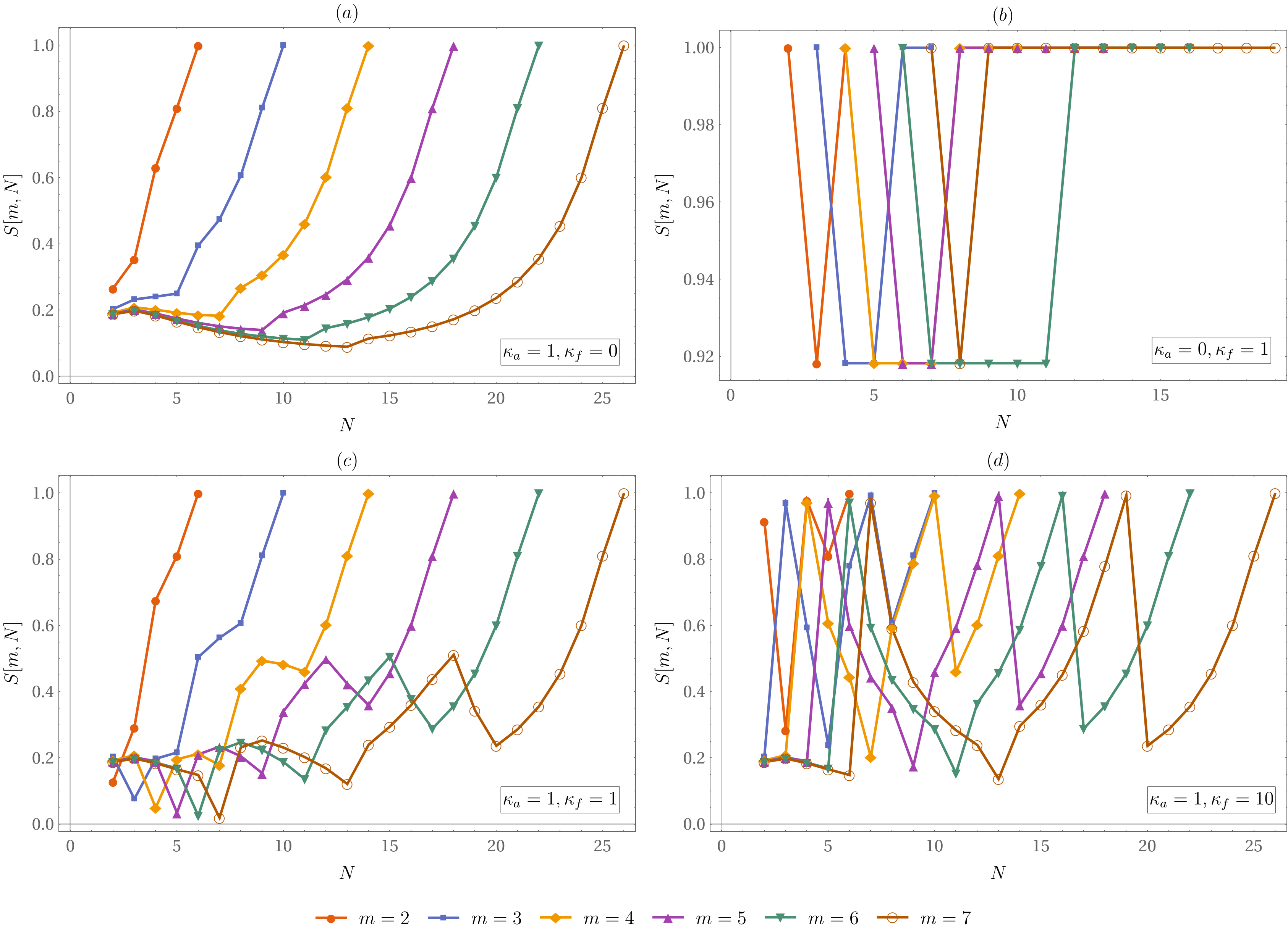
As expected, the entropy varies with the statistical parameter $m$ and the number of particles $N$ .

In Fig 1 a, we plot the entropy corresponding to the anyonic hopping model by setting $\kappa_{a}=1$ and $\kappa_{f}=0$ . In this plot a transition point is observed at $N=2m-1$ . When $N\leq 2m-1$ , the number of configurations (dimension of the $N$ -particle Hilbert space) increases linearly with $N$ . But, it decreases linearly with $N$ for $N>2m-1$ since the maximum occupancy at a given lattice site is limited to $2m-1$ . This transition at $N=2m-1$ is reflected in the entropy.

In Fig 1 b, we plot the entropy corresponding to the fermionic hopping model by setting $\kappa_{a}=0$ and $\kappa_{f}=1$ . For each constant value of $m$ , we plot the entropy against $N$ where $m\leq N\leq 3m-2$ . The reason, as mentioned in the last section, is that the $N$ -particle Hamiltonian vanishes if $N<m$ and $N>3m-2$ and hence it is meaningless to define the entropy in these cases. It is observed that the ground state is degenerate in this case and the entropy $S[m,N]$ for a given value of $m$ and $N$ depends on the randomly chosen ground state.

In Fig 1 c and in Fig 1 d, we plot the entropy corresponding to the values $(\kappa_{a}=1,\kappa_{f}=1)$ and $(\kappa_{a}=1,\kappa_{f}=10).$ Note that there are several transition points at different values of $N$ for different values of the statistics parameter $m$ in these plots. These transitions mainly occur at values $N=m$ , $N=2m-1$ , and $N=3m-1$ . The reason for a transition point at $N=2m-1$ is as explained in the case of Fig. 1 a. The transition points at $N=m$ and $N=3m-1$ are related to the number of fermions in the system. As explained before, the entropy does not depend upon the fermionic hopping parameter $\kappa_{f}$ when $N<m$ and $N>3m-2$ since the term vanishes in these limits. The dependence of entropy on the statistics parameter is dominated by the anyonic behaviour as the number of particles is increased, interspersed with jumps associated with fermionic behaviour obtained when the number of anyons completes a fermionic composite.

There are other transitions that happen at different $N$ values. It is not clear if these are an artifact of the numerical calculation, or if there is a deeper physical reason.

5 Conclusions

Composite particles help us to explain various physical phenomena. In the present work, we constructed fermions as composites of anyons in one dimension. These anyons are constructed by generalizing Pauli’s exclusion principle as well as the exchange properties of multiparticle wave functions and are defined by a specific algebra we propose. We studied a model of these anyons defined by a Hamiltonian which consists of hopping terms both for elementary anyons and fermionic composites of anyons. We also studied the quantum entanglement of these anyons. The dependence of the entanglement entropy on the statistics parameter and the number of particles is explored numerically.

Appendix A Number operator

We can derive the following identities using straightforward algebra

$\displaystyle a_{j}^{p}(a_{j}^{\dagger})a_{j}^{q}$	$\displaystyle=a_{j}^{p+q-1}$	(40)
$\displaystyle a_{j}(a_{j}^{\dagger})^{p}$	$\displaystyle=(a_{j}^{\dagger})^{(p-1)}-(a_{j}^{\dagger})^{(\nu)}(a_{j})^{(\nu-(p-1))}$	(41)
$\displaystyle(a_{j})^{q}(a_{j}^{\dagger})^{p}$	$\displaystyle=\delta_{p,q}+\theta_{1}(q-p)(a_{j})^{q-p}+\theta_{1}(p-q)(a_{j}^{\dagger})^{(p-q)}-(a_{j}^{\dagger})^{(\nu-(q-1))}(a_{j})^{(\nu-(p-1))}$	(42)
$\displaystyle a_{j}^{\nu}(a_{j}^{\dagger})^{p}a_{j}^{\nu}$	$\displaystyle=0,~~~p<\nu$	(43)
$\displaystyle a_{j}^{\nu}(a_{j}^{\dagger})^{(\nu)}a_{j}^{\nu}$	$\displaystyle=a_{j}^{\nu}$	(44)

where

\displaystyle\begin{aligned} \theta_{1}(x)=\begin{cases}1&x>0\\ 0&x\leq 0\end{cases}\end{aligned}

(45)

The number density operator is given by

\displaystyle\begin{aligned} n_{j}=\sum_{k=1}^{\nu}(a^{\dagger}_{j})^{k}a_{j}^{k}\end{aligned}

(46)

We compute the commutation relation

\displaystyle\begin{aligned} \left[n_{j},a_{j}\right]&=n_{j}a_{j}-a_{j}n_{j}\\ &=\sum_{k=1}^{\nu-1}(a^{\dagger}_{j})^{k}a_{j}^{k+1}-\sum_{k=1}^{\nu-1}a_{j}(a^{\dagger}_{j})^{k}a_{j}^{k}\\ &=\sum_{k=1}^{\nu-2}(a^{\dagger}_{j})^{k}a_{j}^{k+1}-\sum_{k=1}^{\nu-1}\left((a_{j}^{\dagger})^{(k-1)}-(a_{j}^{\dagger})^{(\nu-1)}(a_{j})^{(\nu-(k-1))}\right)a_{j}^{k}\\ &=\sum_{k=1}^{\nu-2}(a^{\dagger}_{j})^{k}a_{j}^{k+1}-\sum_{k=1}^{\nu-1}(a_{j}^{\dagger})^{(k-1)}a_{j}^{k}\\ &=\sum_{k=1}^{\nu-2}(a^{\dagger}_{j})^{k}a_{j}^{k+1}-\sum_{k=0}^{\nu-2}(a_{j}^{\dagger})^{(k)}a_{j}^{k+1}\\ &=-a_{j}\end{aligned}

(47)

Also,

\displaystyle\begin{aligned} \left[n_{j},a_{k}\right]&=0,~~k\neq j\end{aligned}

(48)

Therefore we obtain the relations

\displaystyle\begin{aligned} \left[n_{j},a_{k}\right]=-\delta_{j,k}a_{k},~~~~\left[n_{j},a_{k}^{\dagger}\right]=\delta_{j,k}a_{k}^{\dagger}\end{aligned}

(49)

The total number operator

\hat{N}=\sum_{i}{n_{i}}

(50)

and

\left[\hat{N},a_{k}\right]=-a_{k},~~~~\left[\hat{N},a_{k}^{\dagger}\right]=a_{k}^{\dagger}

(51)

Appendix B Distribution function

We consider a free gas of anyons in the grand canonical ensemble described by the Hamiltonian

\displaystyle\begin{aligned} H=\sum_{j}\epsilon_{j}n_{j}\end{aligned}

(52)

\displaystyle\begin{aligned} \braket{n_{j}}&=\frac{1}{Z}\tr(n_{j}e^{-\beta(H-\mu N)})&=\frac{1}{Z}\sum_{p=1}^{\nu}\tr\left((a^{\dagger}_{j})^{p}a_{j}^{p}e^{-\beta(H-\mu N)}\right)\end{aligned}

(53)

We have

\displaystyle\begin{aligned} \left[\hat{N},(a_{k}^{\dagger})^{p}\right]&=\left[\hat{N},(a_{k}^{\dagger})\right](a_{k}^{\dagger})^{p-1}+(a_{k}^{\dagger})\left[\hat{N},(a_{k}^{\dagger})\right](a_{k}^{\dagger})^{p-2}+..+(a_{k}^{\dagger})^{p-1}\left[\hat{N},(a_{k}^{\dagger})\right]\\ &=p(a_{k}^{\dagger})^{p}.\end{aligned}

(54)

Similarly,

\displaystyle\begin{aligned} \left[H,(a_{k}^{\dagger})^{p}\right]&=p\epsilon_{k}(a_{k}^{\dagger})^{p}.\end{aligned}

(55)

Using these relations

\displaystyle\begin{aligned} \braket{(a^{\dagger}_{j})^{p}a_{j}^{p}}&=\frac{1}{Z}\tr((a^{\dagger}_{j})^{p}a_{j}^{p}e^{-\beta(H-\mu N)})\\ &=\frac{1}{Z}\tr\left(e^{-\beta(H-\mu N)}(a^{\dagger}_{j})^{p}e^{\beta(H-\mu N)}e^{-\beta(H-\mu N)}a_{j}^{p}\right)\\ &=\frac{1}{Z}e^{-\beta p(\epsilon_{j}-\mu)}\tr\left(e^{-\beta(H-\mu N)}a_{j}^{p}(a^{\dagger}_{j})^{p}\right)\\ &=\frac{1}{Z}e^{-\beta p(\epsilon_{j}-\mu)}\tr\left(e^{-\beta(H-\mu N)}\left(1-(a_{j}^{\dagger})^{(\nu-(p-1))}(a_{j})^{(\nu-(p-1))}\right)\right)\\ &=e^{-\beta p(\epsilon_{j}-\mu)}\left(1-\braket{(a_{j}^{\dagger})^{(\nu-(p-1))}(a_{j})^{(\nu-(p-1))}}\right).\end{aligned}

(56)

We made use of the relation

\displaystyle\begin{aligned} a_{j}^{p}(a^{\dagger}_{j})^{p}&=1-(a_{j}^{\dagger})^{(\nu-(p-1))}(a_{j})^{(\nu-(p-1))}\end{aligned}

(57)

This gives

\displaystyle\begin{aligned} \braket{(a^{\dagger}_{j})^{(\nu-(p-1))}a_{j}^{(\nu-(p-1))}}&=e^{-\beta{(\nu-(p-1))}(\epsilon_{j}-\mu)}\left(1-\braket{(a_{j}^{\dagger})^{p}(a_{j})^{p}}\right).\end{aligned}

(58)

The term

\displaystyle\begin{aligned} \braket{(a^{\dagger}_{j})^{p}a_{j}^{p}}&=e^{-\beta p(\epsilon_{j}-\mu)}-e^{-\beta p(\epsilon_{j}-\mu)}\left(e^{-\beta{(\nu-(p-1))}(\epsilon_{j}-\mu)}-e^{-\beta{(\nu-(p-1))}(\epsilon_{j}-\mu)}\braket{(a_{j}^{\dagger})^{p}(a_{j})^{p}}\right)\\ &=e^{-\beta p(\epsilon_{j}-\mu)}-\left(e^{-\beta{(\nu+1)}(\epsilon_{j}-\mu)}-e^{-\beta{(\nu+1)}(\epsilon_{j}-\mu)}\braket{(a_{j}^{\dagger})^{p}(a_{j})^{p}}\right).\end{aligned}

(59)

Therefore

\displaystyle\begin{aligned} \braket{(a_{j}^{\dagger})^{p}(a_{j})^{p}}\left(1-e^{-\beta{(\nu+1)}(\epsilon_{j}-\mu)}\right)&=e^{-\beta p(\epsilon_{j}-\mu)}-e^{-\beta{(\nu+1)}(\epsilon_{j}-\mu)}\\ \braket{(a_{j}^{\dagger})^{p}(a_{j})^{p}}&=\frac{e^{-\beta p(\epsilon_{j}-\mu)}-e^{-\beta{(\nu+1)}(\epsilon_{j}-\mu)}}{\left(1-e^{-\beta{(\nu+1)}(\epsilon_{j}-\mu)}\right)}\end{aligned}

(60)

Substituting, we get

\displaystyle\begin{aligned} \braket{n_{j}}&=\sum_{p=1}^{\nu}\braket{(a^{\dagger}_{j})^{p}a_{j}^{p}}\\ &=\sum_{p=1}^{\nu}\frac{e^{-\beta p(\epsilon_{j}-\mu)}-e^{-\beta{(\nu+1)}(\epsilon_{j}-\mu)}}{\left(1-e^{-\beta{(\nu+1)}(\epsilon_{j}-\mu)}\right)}\\ &=\frac{\frac{e^{-\beta(\epsilon_{j}-\mu)}-e^{-\beta(\nu+1)(\epsilon_{j}-\mu)}}{1-e^{-\beta(\epsilon_{j}-\mu)}}-\nu e^{-\beta{(\nu+1)}(\epsilon_{j}-\mu)}}{\left(1-e^{-\beta{(\nu+1)}(\epsilon_{j}-\mu)}\right)}\\ &=\frac{1}{\left(e^{\beta(\epsilon_{j}-\mu)}-1\right)}-\frac{(\nu+1)\left(e^{\beta(\epsilon_{j}-\mu)}-1\right)}{\left(e^{\beta{(\nu+1)}(\epsilon_{j}-\mu)}-1\right)}\end{aligned}

(61)

Appendix C Fermionic Algebra

We use the notation $m=\frac{\nu+1}{2}$ where $\nu=1,3,5,..$ and $m\in\mathbb{N}$ . In this notation, the algebraic relations are

\displaystyle\begin{aligned} a_{j}a_{k}&=e^{i\theta\sgn(j-k)}a_{k}a_{j},~k\neq j\\ a_{j}a_{k}^{\dagger}&=e^{-i\theta\sgn(j-k)}a_{k}^{\dagger}a_{j}~k\neq j\\ a_{j}a_{j}^{\dagger}&=1-(a_{j}^{\dagger})^{(2m-1)}(a_{j})^{(2m-1)}\\ a_{j}^{2m}&=0\\ (a_{j}^{\dagger})^{2m}&=0\end{aligned}

(62)

and the identities are

$\displaystyle a_{j}^{p}(a_{j}^{\dagger})a_{j}^{q}$	$\displaystyle=a_{j}^{p+q-1}$	(63)
$\displaystyle a_{j}(a_{j}^{\dagger})^{p}$	$\displaystyle=(a_{j}^{\dagger})^{(p-1)}-(a_{j}^{\dagger})^{(2m-1)}(a_{j})^{(2m-p)}$	(64)
$\displaystyle(a_{j})^{q}(a_{j}^{\dagger})^{p}$	$\displaystyle=\theta_{1}(q-p)(a_{j})^{q-p}+\theta_{1}(p-q)(a_{j}^{\dagger})^{(p-q)}-(a_{j}^{\dagger})^{(2m-q)}(a_{j})^{(2m-p)}$	(65)
$\displaystyle a_{j}^{2m-1}(a_{j}^{\dagger})^{p}a_{j}^{2m-1}$	$\displaystyle=0,~~~p<(2m-1)$	(66)
$\displaystyle a_{j}^{2m-1}(a_{j}^{\dagger})^{(2m-1)}a_{j}^{2m-1}$	$\displaystyle=a_{j}^{2m-1}$	(67)

We define the fermionic operators

\displaystyle\begin{aligned} f_{j}=a_{j}^{m}\end{aligned}

(68)

Since $a_{j}^{2m}=0$ , we have

\displaystyle\begin{aligned} f_{j}^{2}=0.\end{aligned}

(69)

Also we derive the commutation relation

\displaystyle\begin{aligned} f_{j}f_{k}&=a_{j}^{m}a_{k}^{m}\\ &=e^{im\theta\sgn(j-k)}a_{k}a_{j}^{m}a_{k}^{m-1}\\ &=e^{im^{2}\theta\sgn(j-k)}a_{k}^{m}a_{j}^{m}\end{aligned}

(70)

We choose $\theta=\frac{\pi}{m^{2}}$ . This implies

\displaystyle f_{j}f_{k}=-f_{k}f_{j}

(71)

Also,

\displaystyle\begin{aligned} f_{j}f^{\dagger}_{k}&=a_{j}^{m}(a_{k}^{\dagger})^{m}\\ &=e^{-im^{2}\theta\sgn(j-k)}(a_{k}^{\dagger})^{m}a_{j}^{m}\\ &=e^{-i\pi\sgn(j-k)}(a_{k}^{\dagger})^{m}a_{j}^{m}\\ &=-f^{\dagger}_{k}f_{j}\end{aligned}

(72)

Similarly, the other relations can be derived

\displaystyle\begin{aligned} f_{j}f^{\dagger}_{j}&=a_{j}^{m}(a_{j}^{\dagger})^{m}\\ &=1-(a_{j}^{\dagger})^{(m)}a_{j}^{(m)}\\ &=1-f_{j}^{\dagger}f_{j}\end{aligned}

(73)

Hence, $f_{j}$ and $f_{j}^{\dagger}$ satisfy fermionic algebra.

Appendix D Matrix representation of the Hamiltonian

The Hamiltonian for the two-site case is given by

\displaystyle\begin{aligned} H&=H_{a}+H_{f}\\ H_{a}&=-\kappa_{a}\left(a_{1}^{\dagger}a_{2}+a_{2}^{\dagger}a_{1}\right)\\ H_{f}&=-\kappa_{f}\left((a_{1}^{\dagger})^{m}(a_{2})^{m}+(a_{2}^{\dagger})^{m}(a_{1})^{m}\right)\end{aligned}

(74)

We choose the following basis for the Fock space

\displaystyle\begin{aligned} \{|r,s\rangle\},~~~r,s=0,1,2,..,\nu\end{aligned}

(75)

where $|r,s\rangle=(a^{\dagger}_{1})^{r}(a^{\dagger}_{2})^{s}|0\rangle$ . For general $\nu$ there will be $\nu^{2}$ basis states when we consider two lattice sites.

We can express the Hamiltonian in the matrix form in the basis given above

\displaystyle\begin{aligned} H_{q,p;r,s}&=\langle q,p|H|r,s\rangle=\braket{0|a_{2}^{p}a_{1}^{q}H(a^{\dagger}_{1})^{r}(a^{\dagger}_{2})^{s}|0}\end{aligned}

(76)

We have the following matrix elements

\displaystyle\begin{aligned} \langle q,p|(a^{\dagger}_{1})(a_{2})|r,s\rangle&=\langle 0|a_{2}^{p}a_{1}^{q}(a^{\dagger}_{1})(a_{2})(a^{\dagger}_{1})^{r}(a^{\dagger}_{2})^{s}|0\rangle\\ &=e^{\frac{i\pi}{m^{2}}}e^{-\frac{i\pi q}{m^{2}}}\langle 0|a_{2}^{p+1}a_{1}^{q}(a^{\dagger}_{1})^{r+1}(a^{\dagger}_{2})^{s}|0\rangle\\ &=e^{\frac{i\pi(1-q)}{m^{2}}}\delta_{q,r+1}\delta_{p+1,s}\\ &=e^{-\frac{i\pi r}{m^{2}}}\delta_{q,r+1}\delta_{p+1,s}\\ \langle q,p|(a^{\dagger}_{2})(a_{1})|r,s\rangle&=e^{\frac{i\pi(r-1)}{m^{2}}}\delta_{q+1,r}\delta_{p,s+1}\\ \langle q,p|(a^{\dagger}_{1})^{m}(a_{2})^{m}|r,s\rangle&=e^{\frac{i\pi(r-1)}{m^{2}}}\delta_{q+1,r}\delta_{p,s+1}\\ \langle q,p|(a^{\dagger}_{2})^{m}(a_{1})^{m}|r,s\rangle&=e^{\frac{i\pi m(r-1)}{m^{2}}}\delta_{q+m,r}\delta_{p,s+m}\end{aligned}

(77)

Using the above results, the matrix elements of the Hamiltonian are

\displaystyle\begin{aligned} H_{q,p;r,s}=\langle q,p|H|r,s\rangle&=-\kappa_{a}\left(e^{\frac{i\pi(1-q)}{m^{2}}}\delta_{q,r+1}\delta_{p+1,s}+e^{\frac{i\pi(r-1)}{m^{2}}}\delta_{q+1,r}\delta_{p,s+1}\right)\\ &-\kappa_{f}\left(e^{\frac{i\pi m(1-q)}{m^{2}}}\delta_{q,r+m}\delta_{p+m,s}+e^{\frac{i\pi m(r-1)}{m^{2}}}\delta_{q+m,r}\delta_{p,s+m}\right)\end{aligned}

(78)

References

[1] Risto Raitio. A Model of Lepton and Quark Structure. Physica Scripta, 22(3):197–198, January 1980.
[2] Joseph Gerard Polchinski. String Theory, Volume I: An Introduction to the Bosonic String. Cambridge university press Cambridge, 1998.
[3] Leon N. Cooper. Bound Electron Pairs in a Degenerate Fermi Gas. Physical Review, 104(4):1189–1190, November 1956.
[4] Monique Combescot, Odile Betbeder-Matibet, and François Dubin. The many-body physics of composite bosons. Physics Reports, 463(5):215–320, July 2008.
[5] Charles Kittel and Ching-yao Fong. Quantum Theory of Solids. Wiley, 1987.
[6] SM Girvin and R Prange. The Quantum Hall Effect. Springer, New York, 1987.
[7] J. K. Jain. Composite-fermion approach for the fractional quantum Hall effect. Physical Review Letters, 63(2):199–202, July 1989.
[8] Frank Wilczek. Fractional Statistics and Anyon Superconductivity, volume 5. World scientific, 1990.
[9] J. M. Leinaas and J. Myrheim. On the theory of identical particles. Il Nuovo Cimento B (1971-1996), 37(1):1–23, January 1977.
[10] G Gentile j. Itosservazioni sopra le statistiche intermedie. Il Nuovo Cimento (1924-1942), 17:493–497, 1940.
[11] H. S. Green. A Generalized Method of Field Quantization. Physical Review, 90(2):270–273, April 1953.
[12] O. W. Greenberg. Example of infinite statistics. Physical Review Letters, 64(7):705–708, February 1990.
[13] F. D. M. Haldane. “Fractional statistics” in arbitrary dimensions: A generalization of the Pauli principle. Physical Review Letters, 67(8):937–940, August 1991.
[14] Rosario Lo Franco and Giuseppe Compagno. Quantum entanglement of identical particles by standard information-theoretic notions. Scientific reports, 6:20603, 2016.
[15] AP Balachandran, TR Govindarajan, Amilcar R de Queiroz, and AF Reyes-Lega. Algebraic approach to entanglement and entropy. Physical Review A, 88(2):022301, 2013.
[16] GianCarlo Ghirardi and Luca Marinatto. Identical particles and entanglement. Optics and Spectroscopy, 99(3):386–390, 2005.
[17] John Schliemann, J Ignacio Cirac, Marek Kuś, Maciej Lewenstein, and Daniel Loss. Quantum correlations in two-fermion systems. Physical Review A, 64(2):022303, 2001.
[18] R Paškauskas and L You. Quantum correlations in two-boson wave functions. Physical Review A, 64(4):042310, 2001.
[19] Howard Mark Wiseman and John A Vaccaro. Entanglement of indistinguishable particles shared between two parties. Physical review letters, 91(9):097902, 2003.
[20] N Killoran, M Cramer, and Martin B Plenio. Extracting entanglement from identical particles. Physical review letters, 112(15):150501, 2014.
[21] Rosario Lo Franco and Giuseppe Compagno. Indistinguishability of elementary systems as a resource for quantum information processing. Physical review letters, 120(24):240403, 2018.
[22] Fabio Benatti, Roberto Floreanini, and Kelvin Titimbo. Entanglement of identical particles. Open Systems & Information Dynamics, 21(01n02):1440003, 2014.
[23] J. Hubbard and Brian Hilton Flowers. Electron correlations in narrow energy bands. Proceedings of the Royal Society of London. Series A. Mathematical and Physical Sciences, 276(1365):238–257, November 1963.
[24] N Ramadas and VV Sreedhar. Quantum entanglement in the one-dimensional anyonic Hubbard model. Annals of Physics, 442(0003-4916):168908, 2022.
[25] Silvia Noschese, Lionello Pasquini, and Lothar Reichel. Tridiagonal Toeplitz matrices: Properties and novel applications. Numerical Linear Algebra with Applications, 20(2):302–326, 2013.