Can the Higgs Still Account for the Anomaly?
Abstract
We use an Effective Field Theory (EFT) approach to evaluate the viability of the Higgs to account for the anomaly. Although the SM contribution of the Higgs to the muon’s magnetic dipole moment is negligible, using a bottom-up EFT, we show that given the current level of experimental limits on the Higgs sector, the Higgs can still yield a viable solution to the anomaly if its couplings to the rest of the SM particles are allowed to deviate from their SM predictions. Such a solution would only require an fine-tuning. Further, applying unitarity arguments, we show that such a solution would indicate a scale of New Physics (NP) of TeV, which could be lowered to TeV if the Higgs couplings to the and are assumed to conform to their SM predictions. We show that such a scenario could yield significant enhancement to the di-Higgs production in muon colliders, thus providing further motivation for its consideration. A key takeaway of this study is to highlight the importance of measuring the coupling in future experiments.
I Introduction
The anomalous magnetic dipole moment of the muon, known as the anomaly, remains one of the best hints for physics Beyond the Standard Model (BSM). The E821 experiment at BNL Muong-2:2006rrc first showed a discrepancy compared with the theoretical predictions, at a significance of . This was confirmed in 2021 by the E989 experiment at Fermilab Muong-2:2021ojo; Muong-2:2021ovs; Muong-2:2021vma, which yielded a measurement of . The Fermilab measurement, in comparison with the latest theoretical SM prediction of Aoyama:2020ynm; Davier:2017zfy; Keshavarzi:2018mgv; Colangelo:2018mtw; Hoferichter:2019mqg; Davier:2019can; Keshavarzi:2019abf; Kurz:2014wya; FermilabLattice:2017wgj; Budapest-Marseille-Wuppertal:2017okr; RBC:2018dos; Giusti:2019xct; Shintani:2019wai; FermilabLattice:2019ugu; Gerardin:2019rua; Aubin:2019usy; Giusti:2019hkz; Melnikov:2003xd; Masjuan:2017tvw; Colangelo:2017fiz; Hoferichter:2018kwz; Gerardin:2019vio; Bijnens:2019ghy; Colangelo:2019uex; Pauk:2014rta; Danilkin:2016hnh; Jegerlehner:2017gek; Knecht:2018sci; Eichmann:2019bqf; Roig:2019reh; Colangelo:2014qya; Blum:2019ugy; Aoyama:2012wk; Aoyama:2019ryr; Czarnecki:2002nt; Gnendiger:2013pva, further increases the discrepancy to
| (1) |
On the other hand, some of the latest high-precision QCD lattice simulations Borsanyi:2020mff; Ce:2022kxy; Alexandrou:2022amy appear to agree with the experimental measurements, thus reducing the anomaly. However, these results could be in conflict with the data Colangelo:2022vok; DiLuzio:2021uty. This discrepancy arises mainly from the Hadronic Vacuum Polaization (HVP) corrections, which are difficult to calculate (see for instance Crivellin:2020zul; Keshavarzi:2020bfy; Colangelo:2020lcg). Therefore, it seems that further confirmation is needed. On the other hand, a new measurement of the cross section of from the CMD-3 group CMD-3:2023alj, reveals a larger contribution to compared to the previous values in the literature, which makes closer to the experimental value, thereby lowering the significance of the discrepancy in the data-driven approach as well. Nonetheless, this result too is inconsistent with the previous results in the literature and still needs independent corroboration.
The upcoming runs of the E989 experiment are expected to lower the uncertainty by a factor of 4, whereas the E34 collaboration at J-PARC Saito:2012zz; Mibe:2011zz; Abe:2019thb plans on measuring using a completely different method. As for the SM predictions, various theory and lattice groups are expected to present updated results from those in Borsanyi:2020mff; Ce:2022kxy; Alexandrou:2022amy. For the purposes of this study, we will assume that the anomaly exists and is given by eq. (1).
We should also point out that another discrepancy between the predicted and measured magnetic dipole moments of the electron was reported, however, there is disagreement between the two experiments that reported the discrepancy on the sign and significance of the electron anomaly. The first group Aoyama:2019ryr reported an electron anomaly corresponding to a significance of , whereas the second group Morel:2020dww reported , corresponding to a significance of only . Given this disagreement, it is not clear whether the electron anomaly indeed exists or not, and if it does which sign it has. As the sign of the discrepancy is crucial in determining the nature of the physics behind the anomaly, we will ignore it in this work, waiting for more accurate measurements to be made, and for an agreement to be reached.
In this paper, we seek to investigate whether or not the Higgs boson can still accommodate a solution to the anomaly for the muon. In the SM, the contribution of the Higgs to at one loop is and is thus negligible, however, the current level of experimental bounds on the Higgs couplings to the rest of the SM particles still leaves ample room for significant deviation from the SM predictions. For instance, the coupling of the Higgs to is only constrained at , whereas higher-dimensional Higgs operators remain essentially unconstrained. This suggests using an EFT approach in the Higgs interaction with the muon, in order to determine whether or not the muon anomaly can still be solved by the Higgs boson within the experimental constraints. The strategy is simple: We write down the most general Higgs interactions with the muon, and then calculate its contribution to given the experimental constraints, then we determine whether this contribution can account for the measured discrepancy in eq. (1) or not. Similar work using the Standard Model EFT (SMEFT) already exists in the literature Buttazzo:2020ibd; Yin:2020afe; Fajfer:2021cxa; Aebischer:2021uvt; Allwicher:2021jkr; Cheung:2021iev, however, here we utilize a more phenomenologically-transparent, completely model-independent approach Chang:2019vez; Abu-Ajamieh:2020yqi; Abu-Ajamieh:2021egq; Abu-Ajamieh:2022ppp; Abu-Ajamieh:2021vnh in order to calculate the Higgs BSM contributions to the anomaly. We find that given the current level of experimental constraints, the Higgs sector can still provide a solution to the muon anomaly. We show that the viable part of the parameter space can be significantly probed by future experiments, especially the proposed -TeV muon collider MuonCollider:2022cre.
This paper is organized as follows: In Sec. II, we present a review of the model-independent EFT used in Chang:2019vez; Abu-Ajamieh:2020yqi; Abu-Ajamieh:2021egq; Abu-Ajamieh:2022ppp; Abu-Ajamieh:2021vnh; Abu-Ajamieh:2023qvh. In Sec. III, we present the contributions to in this framework at 1 and 2 loops, and we present the current experimental bounds and future projections on the parameter space. In Sec. IV we discuss the phenomenological implications of the model. In Sect. V, we introduce a simple UV extension that can be matched to the EFT, and finally we conclude in Sec. VI.
II Overview of the Model-independent EFT
In this paper, we adopt the EFT framework employed in Chang:2019vez; Abu-Ajamieh:2020yqi; Abu-Ajamieh:2021egq; Abu-Ajamieh:2022ppp; Abu-Ajamieh:2021vnh; Abu-Ajamieh:2023qvh. In this framework, we avoid any power expansion in writing down higher-dimensional operators, as is the case in the SMEFT. Instead, we parameterize NP as deviations from the SM predictions. Therefore, we write the effective Lagrangian of the Yukawa interaction of the lepton sector as follows11 1 This methodology of expanding the Higgs couplings, is reminiscent of the chiral expansion of the Higgs Lagrangian (see for example,Buchalla:2020kdh and the references therein).
| (2) |
where parameterize the deviations of the leptons’ Yukawa couplings compared to the SM predictions
| (3) |
whereas are Wilson coefficients that do not have SM counterparts. The field is defined in terms of the Higgs doublet as
| (4) |
whereas we define the projector , with
| (5) |
where are the Goldstone bosons. Notice that we are dividing by the appropriate powers of only to keep the Wilson coefficients dimensionless, i.e., is NOT an expansion parameter. Notice that in the unitary gauge, and the Goldstone bosons are eaten. In this paper, we simplify our calculations by working in the unitary gauge. Therefore, in this gauge, the Lagrangian in terms of the physical masses becomes
| (6) |
and for the case of the muon . Before we proceed, a couple of remarks are in order. First, we are assuming that is the minimum of the Higgs potential including all higher-order corrections, i.e., GeV, and second, although eq. (6) appears similar to the Higgs EFT (HEFT) Grinstein:2007iv, we should keep in mind that secretly we are using the Higgs doublet in our expansion, and one can easily demonstrate that the effective Lagrangian in eqs. (2) and (6) can be mapped to any expansion in either the SMEFT or the HEFT (see Abu-Ajamieh:2020yqi; Abu-Ajamieh:2021egq; Abu-Ajamieh:2022ppp; Abu-Ajamieh:2021vnh for the matching to the SMEFT operators). In other words, the deviations and Wilson coefficients in eqs. (2) and (6) can receive corrections from any number of higher-order operators in either the SMEFT or the HEFT frameworks. The benefit of this construction is twofold. First: there are fewer assumptions in this framework compared to either the SMEFT or the HEFT. Namely, we are only assuming that there are no light degrees of freedom below the energy scale where the EFT breaks down, and that the deviations and Wilson coefficients are compatible with experimental measurements. The second benefit lies in the fact that parameterizing NP this way is more phenomenologically-transparent, as these deviations and Wilson coefficients are what is measured experimentally as opposed to any expansion scale.
III The BSM contributions to
With eq. (6) in hand, we can readily calculate the BSM contributions to with , treating the effective couplings as contact terms. In our calculation, we limit ourselves to 2 loops. The Feynman diagrams that contribute to the anomaly at one and two loops are shown in Fig. 1. Diagram I has already been calculated in the SM case Jackiw:1972jz (see also Tucker-Smith:2010wdq; Chen:2015vqy). Thus, the BSM contribution can be readily calculated simply by substituting . Given the latest bounds on ATLAS:2019nkf
| (7) |


it is easy to show that this contribution is at most and thus is negligible. Diagram II is loop-suppressed compared to diagram I and therefore is also negligible. Diagrams III and IV (of the Barr-Zee type) have also been calculated before in the SM Czarnecki:1995sz; Haestier:2006mg; Gribouk:2005ee; Gnendiger:2013pva; Czarnecki:1995wq. Therefore, we can immediately extend the results to the BSM case with the above rescaling
| (8) | |||
| (9) |
where and . Notice here that in the fermion loop in diagram IV, only the contributions from are retained. Also notice in the same diagram that the BSM contribution could include the deviations in the Yukawa couplings of the above fermions, namely and , however, given the bounds on these deviations, we checked that their contribution to is insignificant, even if we saturate all experimental bounds and arrange for all the corresponding contributions to conspiratorially add up. Therefore, we set .
Figure 2: The parameter space that corresponds to the solution to , together with the LHC constraints (solid red), the HL-LHC projections (dotted red), and the muon collider projections (dotted blue) on , superimposed. is unconstrained.
Diagram V only depends , and explicit calculation of its contribution shows that it is of when the bound in eq. 7 is saturated. On the other hand, the contribution from diagram VI depends on both and and therefore could be significant. Nonetheless, we checked that compared to the other diagrams, the contribution is suppressed and does not exceed at best, and thus can safely be neglected.
This leaves us with diagrams VII and VIII. Both diagrams are somewhat complicated, however, if we use a UV-cutoff scheme such that , then one can show that they can be approximated by
| (10) | |||||
| (11) |
Here we note in passing that we are only using a UV cutoff scheme for convenience, and using dimensional regularization yields similar results if the renormalization scale is defined appropriately. The results are insensitive to the choice of the renormalization scheme or the UV cutoff/ renormalization scale, as the divergence is only logarithmic. Putting all pieces together, the total BSM contribution to is thus given by
| (12) |
We have 3 parameters, namely , and . In the rest of this paper, we fix TeV. Now, we can use eq. (12) in order to find the region in the parameter space that corresponds to solving the anomaly in eq. 1. Figure 2 shows the viable parameter space that corresponds to the solution to . The plot also shows the experimental constraints given in eq. 7 in solid red. The plot shows that the Higgs sector can still accommodate a solution to the anomaly. This is mainly because the BSM Wilson coefficient is essentially unconstrained experimentally, and we can see that a solution to the anomaly is still possible even if . On the other hand, cannot on its own solve the anomaly if . In fact, we can see that only mildly affects , which is hardly surprising given the smallness of the muon Yukawa coupling and the bound in eq. 7.
The size of required to solve the anomaly is , which might seem large, however, we should keep in mind that this is merely an artifact of our parameterization when we divided by to keep it dimensionless. We should note that with proper power counting (such as in the SMEFT), is divided by a larger UV scale that is typically which would yield lower values of . We shall show later on that perturbativity is maintained for this range of up to safe levels. In addition, we shall discuss the fine-tuning associated with it in the next section.
| HL-LHC | HE-LHC | ILC | CLIC | CEPC | FCC-ee | FCC | Muon (10 TeV) | |
| S2 S2′ | 250 500 1000 | 380 1500 3000 | 240 365 | (ee/eh/hh) | +125 GeV | |||
The current LHC bound in eq. 7 is not very stringent, however, there are many proposed future experiments that are expected to probe the viable parameter space almost fully. These are summarized in Table 1. We show the most relevant ones in Figure 2, which are the HL-LHC projections and the projections from the proposed muon collider with COM runs of . We can see from the plot that the proposed muon collider can essentially probe the entire range of . However, even in this scenario, the Higgs sector remains viable as a potential solution to the anomaly, because remains unconstrained. To the best of our knowledge, there aren’t any proposed measurements of either currently in the LHC or in the future. We think that current and future experiments should probe this effective coupling both because it can potentially provide a solution to the anomaly, even when ; and because of its potential enhancement of the di-Higgs production as we will show below.
IV Phenomenological implications
In this section, we will discuss the phenomenological implications of the viable parameter space, including the implications of nonzero and on unitarity; corrections to the muon mass and the corresponding fine-tuning, the impact on other couplings; and the enhancement to the di-Higgs production.
IV.1 Unitarity-Violation and the Scale of New Physics
As explained in detail in Chang:2019vez; Abu-Ajamieh:2020yqi; Abu-Ajamieh:2021egq; Abu-Ajamieh:2022ppp; Abu-Ajamieh:2021vnh, any non-vanishing deviations from the SM predictions will eventually lead to a breakdown in unitarity at some high energy scale. This is because the SM is the unique UV-complete theory with the observed particle content, and any deviation from the SM predictions will lead to UV-incompleteness that manifests itself as processes with energy-growing amplitudes that eventually lead to a breakdown in unitarity at some high energy scale, which signals the onset of NP.
This implies that each point in the parameter space that corresponds to will point to an energy scale where unitarity is violated, and thus to the scale at which NP should come into play. It is fairly easy to adapt the results of the top sector in Abu-Ajamieh:2022ppp to the muon sector. There is only one model-independent process, namely
| (13) |
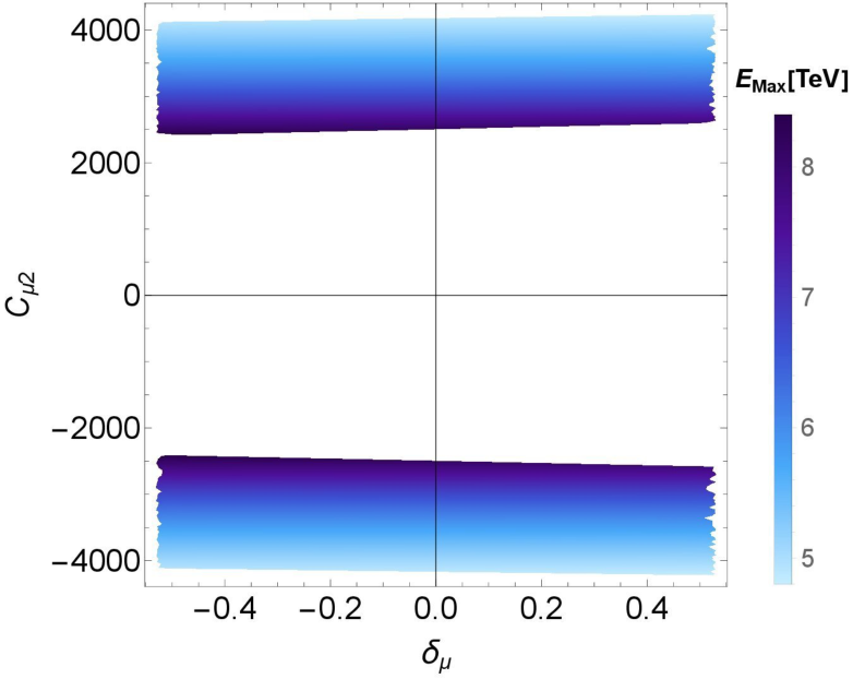
This process is model-independent because it only depends on one parameter, i.e. , and thus the scale of NP is independent of any other assumptions regarding the other potential deviations in the SM. We show the scale of NP that corresponds to the parameter space obtained from eq. 13 on the left side of Figure 3. We can see from the plot that the scale of NP is TeV, which could be probed in the LHC, although if the scale of NP lies at the higher end, this might be difficult. However, this is well within the range of the future -TeV collider, and possibly the proposed muon collider.
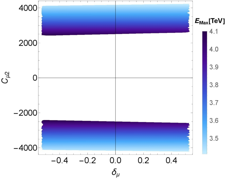
Better bounds, however, can be obtained if the deviations in the couplings of the Higgs to the massive gauge bosons are assumed to vanish. As shown in Abu-Ajamieh:2022ppp, there are other process that violate unitarity, however, the amplitudes of these processes also receive contamination from the deviation in and couplings, with being the or the . Therefore, the scale of NP will also depend on the sizes of these deviations. However, if these deviations are assumed to vanish, then these processes will become functions of and only, which enables us to obtain a lower scale of NP. Up to 6-body scattering, these processes include33 3 We refer the interested reader to Abu-Ajamieh:2022ppp for a complete discussion of how these bounds are obtained from unitarity.
| (14) | |||||
| (15) | |||||
| (16) | |||||
| (17) | |||||
| (18) |
where are the longitudinal modes of the boson. We plot the lowest unitarity-violating scale from eqs. (14-18) on the right-hand side of Figure 3. We can see now that the scale of NP drops to TeV, which is indeed within the reach of the LHC. This suggests that the HL-LHC could shed more light on the potential BSM physics in the Higgs sector and its potential solution of the anomaly.
IV.2 Corrections to the Muon Mass and Fine-tuning
Nonzero and/or will yield corrections to the muon mass. Given the bound in eq. 7, it is easy to see that will at most lead to a mass correction , and thus to fine-tuning . On the other hand, the required size of to solve the anomaly is larger, and thus the corresponding mass correction could be significantly larger.
The correction to the muon mass due to arises when the Higgs loop is closed. Thus, calculating the mass correction can easily be done by integrating out that loop. The corresponding fine-tuning can be estimated as
| (19) |
Given that the size of required to solve the anomaly is , is is easy to see that although the fine-tuning is larger in this case, it is nonetheless still of , and thus remains acceptable.
IV.3 Modification to Muon’s Coupling to the and
The Lagrangian in eq. (2) might suggest that the couplings of the muon to other SM particles might be significantly modified. In particular, when eq. (2) is expressed in a general gauge where the Goldstone bosons are manifest, one would expect from the equivalence theorem, that the coupling of to and will be modified compared to their SM predictions. Nonetheless, here we show that this is not the case, as we are defining the field to be VEV-subtracted as can be seen in eq. (4). To show this explicitly, we write the Higgs doublet in a general gauge
| (20) |
then we insert in eqs. (4) and (5) and expand in powers of , we find
| (21) | |||||
| (22) |
and the eq. (2) becomes
| (23) |
We can expand eq. (23) in powers of , where it is easy to see that at leading order, there is no correction to either or . On the other hand, we could have the effective couplings and . Nonetheless, it is easy to see that even when saturates the bound in es. (7), these couplings are at most, and thus can easily evade any experimental constraints.
IV.4 Di-Higgs Production Enhancement
Nonzero and/or could have interesting phenomenological consequences, such as deviation in the branching fraction of the Higgs decay to , and deviations in the Higgs signal strength from the SM predictions. However, perhaps the most interesting experimental signature for a nonzero and/or is their enhancement of the di-Higgs production. The di-Higgs production provides an excellent probe for NP through both investigating the Higgs couplings compared to the SM, and searching for BSM particles through resonant enhancement, such as additional heavy Higgses, KK gravitons etc. Thus, we confine our discussion to the potential enhancement of the di-Higgs production.
Figure 4: The cross-section of the di-Higgs production in the proposed -TeV muon collider as a function of . The red dashed lines bound the region of the parameter space that corresponds to solving the anomaly.
The strongest enhancement of the di-Higgs production through nonzero and/or arises in muon colliders. In a muon collider, the di-Higgs production proceeds at tree-level and is therefore expected to be sizable. Specifically, proceeds through the and channels, in addition to the contact term. The and channels are proportional to alone and are negligible. On the other hand the contact term depends on and can be sizable. Its cross-section is given by
| (24) |
In Figure 4, we show the cross-section of the di-Higgs production in the proposed -TeV muon collider. The plot shows that for the region of the parameter space that corresponds to the solution to the anomaly, the di-Higgs production cross-section is pb, which is quite sizable. This could be the smoking gun for the viability of the Higgs solution to the anomaly, and it indeed represents another motivation for building the muon collider.
V A Possible UV Model
So far, we have followed a completely bottom-up model-independent approach without reference to any UV completions. Similar work has been discussed in the literature using the SMEFT, see for instance Dermisek:2022aec, where it was argued that any new interaction that results in a chirally-enhanced contribution to , necessarily modifies the decay rate of the Higgs to , or leads to an electric dipole moment for the muon.
In our paper, we have seen that a proper solution would require sizable contributions to the , while at the same time keep the contribution to small to evade the LHC constraints in eq. (7). Building such a model is challenging as it would require conspiratorial cancellations to achieve such a requirement. Here we present a model than can achieve this using vectorlike leptons. The use of vectorlike leptons to solve the anomaly is not new, and has been studied extensively in the literature (see for instance Dermisek:2021mhi; Kannike:2011ng; Dermisek:2013gta; Poh:2017tfo; Dermisek:2021ajd; Arkani-Hamed:2021xlp).
We adopt a model similar to the one presented in Dermisek:2021ajd. The SM is extended by two vectorlike doublets and two vectorlike singlets . and have the same quantum numbers as the SM leptons. In addition, we also introduce a heavy Higgs-like scalar doublet that develops a VEV
| (25) |
![[Uncaptioned image]](2209.10898v4/UV.png) Figure 5: The relevant UV processes. After integrating out the fields and , we obtain the effective Lagrangian in eq. (27).
Figure 5: The relevant UV processes. After integrating out the fields and , we obtain the effective Lagrangian in eq. (27).
The most general Lagrangian can be written as
| (26) |
where we have neglected the interaction of with as they are irrelevant for our purposes. However, we assume that the parameters of the scalar potential are such that they are consistent with experiment. In our model, we set . Assuming that , we can integrate out and (see Figure 5) to arrive at the effective Lagrangian
| (27) |
Defining and matching the Lagrangian in eq. (27) with the effective Lagrangian in eq. (6), we obtain the following matching conditions:
| (28) | |||||
| (29) | |||||
| (30) |
In order to be consistent with experimental measurements, we require that , which leads to
| (31) |
and we can see that we can easily generate the required hierarchy in the scales of the and couplings with TeV. For instance, setting , , we can generate by selecting TeV.
We can see from the proposed UV completion, that maintaining small corrections at LO while allowing for sizable corrections at NLO, would require some conspiratorial cancellations. Nonetheless, one can envisage that such cancellations might arise from a hidden symmetry that protects the LO from receiving large corrections. We will not pursue this issue any further.
VI Conclusions and outlook
In this paper, we analyzed the viability of a BSM Higgs solution to the anomaly using a bottom-up EFT approach. In the SM, the Higgs contribution to the muon’s magnetic dipole moment is negligible. However, given that the current level of experimental limits on the Higgs sector still leaves ample room for NP, it is possible for this contribution to be significantly enhanced compared to the SM.
We saw that while the deviation in the Higgs Yukawa coupling to the muon is not enough to account for the anomaly, the effective coupling , which is unconstrained experimentally, can account for the entire discrepancy. We surveyed the proposed projections on the parameter space and found that the proposed muon collider could provide the best sensitivity for exploring the parameter space. We also showed that unitarity can be used in order to estimate the scale of NP that corresponds to non-vanishing deviations from the SM, i.e. and . We found that the model-independent scale of NP that corresponds to the region of the parameter space that can solve the anomaly to be TeV. This scale is lowered to TeV if the Higgs couplings to massive gauge bosons are assumed to be equal to their SM predictions. We also showed that the corrections to the muon mass that correspond to the size of and required to solve the anomaly, correspond to a fine-tuning level of only.
We also discussed the possible enhancement of the di-Higgs production cross-section, and found that it could be sizable in the proposed TeV muon collider as a result of the contact term interaction through . A key takeaway of this study is that current and future experiments should try to measure and set limits on due to its potential significance in solving the anomaly. Current searches focus of the coupling , which if non-vanishing, is expected to be the largest of the effective couplings of the type . Nonetheless, we believe that should be given similar interest.
In this paper, we confined our analysis to flavor-conserving operators and avoided Flavor Violation (FV). FV Yukawa couplings have been discussed extensively in the literature, see for instance Harnik:2012pb and the references therein, however, to the best of our knowledge, FV effective operators such as have never been properly investigated before, although they were briefly discussed in Babu:1999me; Giudice:2008uua; Goudelis:2011un. We will study these types of FV coupling in a future work.
Acknowledgments
FA would like to that Stephen Martin for the valuable correspondence. The work of FA is supported by the C.V. Raman fellowship from CHEP at IISc. S.K.V. thanks SERB Grant CRG/2021/007170 ”Tiny Effects from Heavy New Physics” from Department of Science and Technology, Government of India.
References
- (1) G. W. Bennett et al. [Muon g-2], “Final Report of the Muon E821 Anomalous Magnetic Moment Measurement at BNL,” Phys. Rev. D 73, 072003 (2006) hep-ex/hep-ex/0602035.
- (2) B. Abi et al. [Muon g-2], “Measurement of the Positive Muon Anomalous Magnetic Moment to 0.46 ppm,” Phys. Rev. Lett. 126, no.14, 141801 (2021) hep-ex/2104.03281.
- (3) T. Albahri et al. [Muon g-2], “Magnetic-field measurement and analysis for the Muon Experiment at Fermilab,” Phys. Rev. A 103, no.4, 042208 (2021) hep-ex/2104.03201.
- (4) T. Albahri et al. [Muon g-2], “Measurement of the anomalous precession frequency of the muon in the Fermilab Muon Experiment,” Phys. Rev. D 103, no.7, 072002 (2021) hep-ex/2104.03247.
- (5) T. Aoyama, N. Asmussen, M. Benayoun, J. Bijnens, T. Blum, M. Bruno, I. Caprini, C. M. Carloni Calame, M. Cè and G. Colangelo, et al. “The anomalous magnetic moment of the muon in the Standard Model,” Phys. Rept. 887, 1-166 (2020) hep-ph/2006.04822.
- (6) M. Davier, A. Hoecker, B. Malaescu and Z. Zhang, “Reevaluation of the hadronic vacuum polarisation contributions to the Standard Model predictions of the muon and using newest hadronic cross-section data,” Eur. Phys. J. C 77, no.12, 827 (2017) hep-ph/1706.09436.
- (7) A. Keshavarzi, D. Nomura and T. Teubner, “Muon and : a new data-based analysis,” Phys. Rev. D 97, no.11, 114025 (2018) hep-ph/1802.02995.
- (8) G. Colangelo, M. Hoferichter and P. Stoffer, “Two-pion contribution to hadronic vacuum polarization,” JHEP 02, 006 (2019) hep-ph/1810.00007.
- (9) M. Hoferichter, B. L. Hoid and B. Kubis, “Three-pion contribution to hadronic vacuum polarization,” JHEP 08, 137 (2019) hep-ph/1907.01556.
- (10) M. Davier, A. Hoecker, B. Malaescu and Z. Zhang, “A new evaluation of the hadronic vacuum polarisation contributions to the muon anomalous magnetic moment and to ,” Eur. Phys. J. C 80, no.3, 241 (2020) [erratum: Eur. Phys. J. C 80, no.5, 410 (2020)] hep-ph/1908.00921.
- (11) A. Keshavarzi, D. Nomura and T. Teubner, “ of charged leptons, , and the hyperfine splitting of muonium,” Phys. Rev. D 101, no.1, 014029 (2020) hep-ph/1911.00367.
- (12) A. Kurz, T. Liu, P. Marquard and M. Steinhauser, “Hadronic contribution to the muon anomalous magnetic moment to next-to-next-to-leading order,” Phys. Lett. B 734, 144-147 (2014) hep-ph/1403.6400.
- (13) B. Chakraborty et al. [Fermilab Lattice, LATTICE-HPQCD and MILC], “Strong-Isospin-Breaking Correction to the Muon Anomalous Magnetic Moment from Lattice QCD at the Physical Point,” Phys. Rev. Lett. 120, no.15, 152001 (2018) hep-lat/1710.11212.
- (14) S. Borsanyi et al. [Budapest-Marseille-Wuppertal], “Hadronic vacuum polarization contribution to the anomalous magnetic moments of leptons from first principles,” Phys. Rev. Lett. 121, no.2, 022002 (2018) hep-lat/1711.04980.
- (15) T. Blum et al. [RBC and UKQCD], “Calculation of the hadronic vacuum polarization contribution to the muon anomalous magnetic moment,” Phys. Rev. Lett. 121, no.2, 022003 (2018) hep-lat/1801.07224.
- (16) D. Giusti, V. Lubicz, G. Martinelli, F. Sanfilippo and S. Simula, “Electromagnetic and strong isospin-breaking corrections to the muon from Lattice QCD+QED,” Phys. Rev. D 99, no.11, 114502 (2019) hep-lat/1901.10462.
- (17) E. Shintani et al. [PACS], “Hadronic vacuum polarization contribution to the muon with 2+1 flavor lattice QCD on a larger than (10 fm lattice at the physical point,” Phys. Rev. D 100, no.3, 034517 (2019) hep-lat/1902.00885.
- (18) C. T. H. Davies et al. [Fermilab Lattice, LATTICE-HPQCD and MILC], “Hadronic-vacuum-polarization contribution to the muon’s anomalous magnetic moment from four-flavor lattice QCD,” Phys. Rev. D 101, no.3, 034512 (2020) hep-lat/1902.04223.
- (19) A. Gérardin, M. Cè, G. von Hippel, B. Hörz, H. B. Meyer, D. Mohler, K. Ottnad, J. Wilhelm and H. Wittig, “The leading hadronic contribution to from lattice QCD with flavours of O() improved Wilson quarks,” Phys. Rev. D 100, no.1, 014510 (2019) hep-lat/1904.03120.
- (20) C. Aubin, T. Blum, C. Tu, M. Golterman, C. Jung and S. Peris, “Light quark vacuum polarization at the physical point and contribution to the muon ,” Phys. Rev. D 101, no.1, 014503 (2020) hep-lat/1905.09307.
- (21) D. Giusti and S. Simula, “Lepton anomalous magnetic moments in Lattice QCD+QED,” PoS LATTICE2019, 104 (2019) hep-lat/1910.03874.
- (22) K. Melnikov and A. Vainshtein, “Hadronic light-by-light scattering contribution to the muon anomalous magnetic moment revisited,” Phys. Rev. D 70, 113006 (2004) hep-ph/0312226.
- (23) P. Masjuan and P. Sanchez-Puertas, “Pseudoscalar-pole contribution to the : a rational approach,” Phys. Rev. D 95, no.5, 054026 (2017) hep-ph/1701.05829.
- (24) G. Colangelo, M. Hoferichter, M. Procura and P. Stoffer, “Dispersion relation for hadronic light-by-light scattering: two-pion contributions,” JHEP 04, 161 (2017) hep-ph/1702.07347.
- (25) M. Hoferichter, B. L. Hoid, B. Kubis, S. Leupold and S. P. Schneider, “Dispersion relation for hadronic light-by-light scattering: pion pole,” JHEP 10, 141 (2018) hep-ph/1808.04823.
- (26) A. Gérardin, H. B. Meyer and A. Nyffeler, “Lattice calculation of the pion transition form factor with Wilson quarks,” Phys. Rev. D 100, no.3, 034520 (2019) hep-lat/1903.09471.
- (27) J. Bijnens, N. Hermansson-Truedsson and A. Rodríguez-Sánchez, “Short-distance constraints for the HLbL contribution to the muon anomalous magnetic moment,” Phys. Lett. B 798, 134994 (2019) hep-ph/1908.03331.
- (28) G. Colangelo, F. Hagelstein, M. Hoferichter, L. Laub and P. Stoffer, “Longitudinal short-distance constraints for the hadronic light-by-light contribution to with large- Regge models,” JHEP 03, 101 (2020) hep-ph/1910.13432.
- (29) V. Pauk and M. Vanderhaeghen, “Single meson contributions to the muon‘s anomalous magnetic moment,” Eur. Phys. J. C 74, no.8, 3008 (2014) hep-ph/1401.0832.
- (30) I. Danilkin and M. Vanderhaeghen, “Light-by-light scattering sum rules in light of new data,” Phys. Rev. D 95, no.1, 014019 (2017) hep-ph/1611.04646.
- (31) F. Jegerlehner, “The Anomalous Magnetic Moment of the Muon,” Springer Tracts Mod. Phys. 274, pp.1-693 (2017) Springer, 2017,
- (32) M. Knecht, S. Narison, A. Rabemananjara and D. Rabetiarivony, “Scalar meson contributions to a from hadronic light-by-light scattering,” Phys. Lett. B 787, 111-123 (2018) hep-ph/1808.03848.
- (33) G. Eichmann, C. S. Fischer and R. Williams, “Kaon-box contribution to the anomalous magnetic moment of the muon,” Phys. Rev. D 101, no.5, 054015 (2020) hep-ph/1910.06795.
- (34) P. Roig and P. Sanchez-Puertas, “Axial-vector exchange contribution to the hadronic light-by-light piece of the muon anomalous magnetic moment,” Phys. Rev. D 101, no.7, 074019 (2020) hep-ph/1910.02881.
- (35) G. Colangelo, M. Hoferichter, A. Nyffeler, M. Passera and P. Stoffer, “Remarks on higher-order hadronic corrections to the muon g2,” Phys. Lett. B 735, 90-91 (2014) hep-ph/1403.7512.
- (36) T. Blum, N. Christ, M. Hayakawa, T. Izubuchi, L. Jin, C. Jung and C. Lehner, “Hadronic Light-by-Light Scattering Contribution to the Muon Anomalous Magnetic Moment from Lattice QCD,” Phys. Rev. Lett. 124, no.13, 132002 (2020) hep-lat/1911.08123.
- (37) T. Aoyama, M. Hayakawa, T. Kinoshita and M. Nio, “Complete Tenth-Order QED Contribution to the Muon g-2,” Phys. Rev. Lett. 109, 111808 (2012) hep-ph/1205.5370.
- (38) T. Aoyama, T. Kinoshita and M. Nio, “Theory of the Anomalous Magnetic Moment of the Electron,” Atoms 7, no.1, 28 (2019)
- (39) A. Czarnecki, W. J. Marciano and A. Vainshtein, “Refinements in electroweak contributions to the muon anomalous magnetic moment,” Phys. Rev. D 67, 073006 (2003) [erratum: Phys. Rev. D 73, 119901 (2006)] hep-ph/0212229.
- (40) C. Gnendiger, D. Stöckinger and H. Stöckinger-Kim, “The electroweak contributions to after the Higgs boson mass measurement,” Phys. Rev. D 88, 053005 (2013) hep-ph/1306.5546.
- (41) S. Borsanyi, Z. Fodor, J. N. Guenther, C. Hoelbling, S. D. Katz, L. Lellouch, T. Lippert, K. Miura, L. Parato and K. K. Szabo, et al. “Leading hadronic contribution to the muon magnetic moment from lattice QCD,” Nature 593, no.7857, 51-55 (2021) hep-lat/2002.12347.
- (42) M. Cè, A. Gérardin, G. von Hippel, R. J. Hudspith, S. Kuberski, H. B. Meyer, K. Miura, D. Mohler, K. Ottnad and P. Srijit, et al. “Window observable for the hadronic vacuum polarization contribution to the muon from lattice QCD,” hep-lat/2206.06582.
- (43) C. Alexandrou, S. Bacchio, P. Dimopoulos, J. Finkenrath, R. Frezzotti, G. Gagliardi, M. Garofalo, K. Hadjiyiannakou, B. Kostrzewa and K. Jansen, et al. “Lattice calculation of the short and intermediate time-distance hadronic vacuum polarization contributions to the muon magnetic moment using twisted-mass fermions,” hep-lat/2206.15084.
- (44) G. Colangelo, A. X. El-Khadra, M. Hoferichter, A. Keshavarzi, C. Lehner, P. Stoffer and T. Teubner, “Data-driven evaluations of Euclidean windows to scrutinize hadronic vacuum polarization,” Phys. Lett. B 833, 137313 (2022) hep-ph/2205.12963.
- (45) L. Di Luzio, A. Masiero, P. Paradisi and M. Passera, “New physics behind the new muon g-2 puzzle?,” Phys. Lett. B 829, 137037 (2022) hep-ph/2112.08312.
- (46) A. Crivellin, M. Hoferichter, C. A. Manzari and M. Montull, “Hadronic Vacuum Polarization: versus Global Electroweak Fits,” Phys. Rev. Lett. 125, no.9, 091801 (2020) hep-ph/2003.04886.
- (47) A. Keshavarzi, W. J. Marciano, M. Passera and A. Sirlin, “Muon and connection,” Phys. Rev. D 102, no.3, 033002 (2020) hep-ph/2006.12666.
- (48) G. Colangelo, M. Hoferichter and P. Stoffer, “Constraints on the two-pion contribution to hadronic vacuum polarization,” Phys. Lett. B 814, 136073 (2021) hep-ph/2010.07943.
- (49) F. V. Ignatov et al. [CMD-3], “Measurement of the cross section from threshold to 1.2 GeV with the CMD-3 detector,” hep-exp/2302.08834.
- (50) N. Saito [J-PARC g-’2/EDM], “A novel precision measurement of muon g-2 and EDM at J-PARC,” AIP Conf. Proc. 1467, 45-56 (2012)
- (51) T. Mibe [J-PARC g-2], “Measurement of muon g-2 and EDM with an ultra-cold muon beam at J-PARC,” Nucl. Phys. B Proc. Suppl. 218, 242-246 (2011)
- (52) M. Abe, S. Bae, G. Beer, G. Bunce, H. Choi, S. Choi, M. Chung, W. Da Silva, S. Eidelman and M. Finger, et al. “A New Approach for Measuring the Muon Anomalous Magnetic Moment and Electric Dipole Moment,” PTEP 2019, no.5, 053C02 (2019) physics.ins-det/1901.03047.
- (53) L. Morel, Z. Yao, P. Cladé and S. Guellati-Khélifa, “Determination of the fine-structure constant with an accuracy of 81 parts per trillion,” Nature 588, no.7836, 61-65 (2020)
- (54) D. Buttazzo and P. Paradisi, “Probing the muon anomaly with the Higgs boson at a muon collider,” Phys. Rev. D 104, no.7, 075021 (2021) hep-ph/2012.02769.
- (55) W. Yin and M. Yamaguchi, “Muon g-2 at a multi-TeV muon collider,” Phys. Rev. D 106, no.3, 033007 (2022) hep-ph/2012.03928.
- (56) S. Fajfer, J. F. Kamenik and M. Tammaro, “Interplay of New Physics effects in (g 2)l and h → +- — lessons from SMEFT,” JHEP 06, 099 (2021) hep-ph/2103.10859.
- (57) J. Aebischer, W. Dekens, E. E. Jenkins, A. V. Manohar, D. Sengupta and P. Stoffer, “Effective field theory interpretation of lepton magnetic and electric dipole moments,” JHEP 07, 107 (2021) hep-ph/2102.08954.
- (58) L. Allwicher, L. Di Luzio, M. Fedele, F. Mescia and M. Nardecchia, “What is the scale of new physics behind the muon g-2?,” Phys. Rev. D 104, no.5, 055035 (2021) hep-ph/2105.13981.
- (59) K. Cheung and Z. S. Wang, “Physics potential of a muon-proton collider,” Phys. Rev. D 103, 116009 (2021) hep-ph/2101.10476.
- (60) S. Chang and M. A. Luty, “The Higgs Trilinear Coupling and the Scale of New Physics,” JHEP 03, 140 (2020) hep-ph/1902.05556.
- (61) F. Abu-Ajamieh, S. Chang, M. Chen and M. A. Luty, “Higgs coupling measurements and the scale of new physics,” JHEP 07, 056 (2021) hep-ph/2009.11293.
- (62) F. Abu-Ajamieh, “The scale of new physics from the Higgs couplings to and Z,” JHEP 06, 091 (2022) hep-ph/2112.13529.
- (63) F. Abu-Ajamieh, “The scale of new physics from the Higgs couplings to gg,” Phys. Lett. B 833, 137389 (2022) hep-ph/2203.07410.
- (64) F. Abu-Ajamieh, “Model-independent Veltman condition, naturalness and the little hierarchy problem *,” Chin. Phys. C 46, no.1, 013101 (2022) hep-ph/2101.06932.
- (65) F. Abu-Ajamieh, M. Frasca and S. K. Vempati, “Flavor Violating Di- Higgs Coupling,” hep-ph/2305.17362.
- (66) D. Stratakis et al. [Muon Collider], “A Muon Collider Facility for Physics Discovery,” physics.acc-ph/2203.08033.
- (67) G. Buchalla, O. Catà, A. Celis, M. Knecht and C. Krause, “Higgs-electroweak chiral Lagrangian: One-loop renormalization group equations,” Phys. Rev. D 104, no.7, 076005 (2021) hep-ph/2004.11348.
- (68) B. Grinstein and M. Trott, “A Higgs-Higgs bound state due to new physics at a TeV,” Phys. Rev. D 76, 073002 (2007) hep-ph/0704.1505.
- (69) R. Jackiw and S. Weinberg, “Weak interaction corrections to the muon magnetic moment and to muonic atom energy levels,” Phys. Rev. D 5, 2396-2398 (1972)
- (70) D. Tucker-Smith and I. Yavin, “Muonic hydrogen and MeV forces,” Phys. Rev. D 83, 101702 (2011) hep-ph/1011.4922.
- (71) C. Y. Chen, H. Davoudiasl, W. J. Marciano and C. Zhang, “Implications of a light “dark Higgs” solution to the -2 discrepancy,” Phys. Rev. D 93, no.3, 035006 (2016) hep-ph/1511.04715.
- (72) G. Aad et al. [ATLAS], “Combined measurements of Higgs boson production and decay using up to fb-1 of proton-proton collision data at 13 TeV collected with the ATLAS experiment,” Phys. Rev. D 101, no.1, 012002 (2020) hep-ex/1909.02845.
- (73) “Electroweak corrections to the muon anomalous magnetic moment,” Phys. Rev. Lett. 76, 3267-3270 (1996) ./hep-ph/9512369
- (74) J. Haestier, S. Heinemeyer, W. Hollik, D. Stockinger, A. M. Weber and G. Weiglein, “Precision Observables in the MSSM: W mass and the muon magnetic moment,” AIP Conf. Proc. 903, no.1, 291-294 (2007) ./hep-ph/0610318
- (75) T. Gribouk and A. Czarnecki, “Electroweak interactions and the muon g-2: Bosonic two-loop effects,” Phys. Rev. D 72, 053016 (2005) ./hep-ph/0509205
- (76) A. Czarnecki, B. Krause and W. J. Marciano, “Electroweak Fermion loop contributions to the muon anomalous magnetic moment,” Phys. Rev. D 52, R2619-R2623 (1995) ./hep-ph/9506256
- (77) J. de Blas, M. Cepeda, J. D’Hondt, R. K. Ellis, C. Grojean, B. Heinemann, F. Maltoni, A. Nisati, E. Petit and R. Rattazzi, et al. “Higgs Boson Studies at Future Particle Colliders,” JHEP 01, 139 (2020) hep-ph/1905.03764.
- (78) F. Abu-Ajamieh, S. Chang, M. Chen, D. Liu and M. A. Luty, “Snowmass 2021 White Paper: Higgs Coupling Sensitivities and Model-Independent Bounds on the Scale of New Physics,” hep-ph/2203.09512.
- (79) S. Dawson, P. Meade, I. Ojalvo, C. Vernieri, S. Adhikari, F. Abu-Ajamieh, A. Alberta, H. Bahl, R. Barman and M. Basso, et al. “Report of the Topical Group on Higgs Physics for Snowmass 2021: The Case for Precision Higgs Physics,” hep-ph/2209.07510.
- (80) A. Azatov, R. Contino, G. Panico and M. Son, “Effective field theory analysis of double Higgs boson production via gluon fusion,” Phys. Rev. D 92, no.3, 035001 (2015) hep-ph/1502.00539.
- (81) R. Harnik, J. Kopp and J. Zupan, “Flavor Violating Higgs Decays,” JHEP 03, 026 (2013) hep-ph/1209.1397.
- (82) K. S. Babu and S. Nandi, “Natural fermion mass hierarchy and new signals for the Higgs boson,” Phys. Rev. D 62, 033002 (2000) hep-ph/hep-ph/9907213.
- (83) G. F. Giudice and O. Lebedev, “Higgs-dependent Yukawa couplings,” Phys. Lett. B 665, 79-85 (2008) hep-ph/0804.1753.
- (84) A. Goudelis, O. Lebedev and J. h. Park, “Higgs-induced lepton flavor violation,” Phys. Lett. B 707, 369-374 (2012) hep-ph/1111.1715.
- (85) R. Dermisek, K. Hermanek, N. McGinnis and S. Yoon, “Ellipse of Muon Dipole Moments,” Phys. Rev. Lett. 129, no.22, 221801 (2022) hep-ph/2205.14243.
- (86) K. Kannike, M. Raidal, D. M. Straub and A. Strumia, “Anthropic solution to the magnetic muon anomaly: the charged see-saw,” JHEP 02, 106 (2012) [erratum: JHEP 10, 136 (2012)] hep-ph/1111.2551.
- (87) R. Dermisek and A. Raval, “Explanation of the Muon g-2 Anomaly with Vectorlike Leptons and its Implications for Higgs Decays,” Phys. Rev. D 88, 013017 (2013) hep-ph/1305.3522.
- (88) Z. Poh and S. Raby, “Vectorlike leptons: Muon g-2 anomaly, lepton flavor violation, Higgs boson decays, and lepton nonuniversality,” Phys. Rev. D 96, no.1, 015032 (2017) hep-ph/1705.07007.
- (89) R. Dermisek, K. Hermanek and N. McGinnis, “Muon g-2 in two-Higgs-doublet models with vectorlike leptons,” Phys. Rev. D 104, no.5, 055033 (2021) hep-ph/2103.05645.
- (90) R. Dermisek, K. Hermanek and N. McGinnis, “Di-Higgs and tri-Higgs boson signals of muon g-2 at a muon collider,” Phys. Rev. D 104, no.9, L091301 (2021) hep-ph/2108.10950.
- (91) N. Arkani-Hamed and K. Harigaya, “Naturalness and the muon magnetic moment,” JHEP 09, 025 (2021) hep-ph/2106.01373.
- (92) A. Crivellin and M. Hoferichter, “Consequences of chirally enhanced explanations of for and ,” JHEP 07, 135 (2021) [erratum: JHEP 10, 030 (2022)] hep-ph]/2104.03202.