Online Ridesharing with Meeting Points
Abstract.
Nowadays, ridesharing becomes a popular commuting mode. Dynamically arriving riders post their origins and destinations, then the platform assigns drivers to serve them. In ridesharing, different groups of riders can be served by one driver if their trips can share common routes. Recently, many ridesharing companies (e.g., Didi and Uber) further propose a new mode, namely “ridesharing with meeting points”. Specifically, with a short walking distance but less payment, riders can be picked up and dropped off around their origins and destinations, respectively. In addition, meeting points enables more flexible routing for drivers, which can potentially improve the global profit of the system. In this paper, we first formally define the Meeting-Point-based Online Ridesharing Problem (MORP). We prove that MORP is NP-hard and there is no polynomial-time deterministic algorithm with a constant competitive ratio for it. We notice that a structure of vertex set, -skip cover, fits well to the MORP. -skip cover tends to find the vertices (meeting points) that are convenient for riders and drivers to come and go. With meeting points, MORP tends to serve more riders with these convenient vertices. Based on the idea, we introduce a convenience-based meeting point candidates selection algorithm. We further propose a hierarchical meeting-point oriented graph (HMPO graph), which ranks vertices for assignment effectiveness and constructs -skip cover to accelerate the whole assignment process. Finally, we utilize the merits of -skip cover points for ridesharing and propose a novel algorithm, namely SMDB, to solve MORP. Extensive experiments on real and synthetic datasets validate the effectiveness and efficiency of our algorithms.
PVLDB Reference Format:
PVLDB, 15(13): XXX-XXX, 2022.
doi:XX.XX/XXX.XX
††
This work is licensed under the Creative Commons BY-NC-ND 4.0 International License. Visit https://creativecommons.org/licenses/by-nc-nd/4.0/ to view a copy of this license. For any use beyond those covered by this license, obtain permission by emailing info@vldb.org. Copyright is held by the owner/author(s). Publication rights licensed to the VLDB Endowment.
Proceedings of the VLDB Endowment, Vol. 15, No. 13 ISSN 2150-8097.
doi:XX.XX/XXX.XX
PVLDB Artifact Availability:
The source code, data, and/or other artifacts have been made available at https://github.com/dominatorX/open.
1. Introduction
Nowadays, on-demand ridesharing becomes important in civil commuting services. Together with online platforms (e.g., DiDi (did 2022)), ridesharing surpasses traditional taxi services with more saved energy, less air pollution, and lower cost (SUMC 2018).
In online ridesharing, riders arrive dynamically. Platforms need to deal with them immediately for different objectives, including maxmizing the number of served riders (Cici et al. 2015; d’Orey et al. 2012; Kleiner et al. 2011; Santos and Xavier 2013; Yeung et al. 2016), minimizing the total travel distance (Alonso-Mora et al. 2017; Gupta et al. 2010; Herbawi and Weber 2012; Huang et al. 2014; Ma et al. 2013; Ota et al. 2017; Rubinstein et al. 2012; Santos and Xavier 2013; Thangaraj et al. 2017), or maximizing the unified revenue (Asghari et al. 2016; Asghari and Shahabi 2017; Tong et al. 2018).
Ridesharing allows one driver to serve more than one group of riders simultaneously. The route of a driver is a sequence of pick-up/drop-off points. Given a set of drivers and riders, route planning is to design and update routes every time a rider arrives. A key operation, called insertion, shows great effectiveness and efficiency for solving online ridesharing problem (Ma et al. 2013; Huang et al. 2014; Thangaraj et al. 2017; Ota et al. 2017; Santos and Xavier 2013; Yeung et al. 2016; Cheng et al. 2017; Cici et al. 2015; Tong et al. 2018). It tries to insert a newly coming rider’s origin and destination into a driver’s route without changing the order of his/her current sequence of pick-up/drop-off points.

However, due to the complex topology of the city road network, some locations are spatially close to each other but hard to access for vehicles. Especially, if two locations are only connected by a Pedestrian Street, where vehicles cannot go through, a short walking could greatly reduce the travel cost of the assigned vehicle. To deal with the case, meeting points (MP for short) are introduced as alternative locations for pick-up/drop-off locations of riders (Stiglic et al. 2015). As shown in Figure 1, a rider at location A wants to go to location C. The nearby roads are directed roads. A driver at location B is assigned to serve . Then, the shortest route for is represented in blue dashed arrow lines. If can move a short distance, for example, to location D (i.e., an MP), can serve through a much shorter route displayed in the green line.
In a recent work (Zhao et al. 2018), the authors utilize meeting points to improve the results of offline ridesharing problems, whose method however is slow and only can handle up to 40 riders/vehicles in real time. Thus, it is not practical for online applications (e.g., Uber and DiDi) with hundreds of riders/vehicles every several seconds. Existing studies also investigate the strategies to properly select MPs with online surveys (Czioska et al. 2017; Eser et al. 2018). In industry, Uber recently offers Express POOL to encourage riders to walk to Express spots (meeting points) for efficient routing (Exp 2019). Nevertheless, Uber Express Pool only schedules the route for each vehicle when there are shareable ride-requests to group with, otherwise, the rider needs to wait until other shareable riders come. In addition, the MPs in Uber Express Pool are similar to the stops of buses for nearby riders to come together and thus not flexible (Ube 2019). For the example in Figure 1, Uber Express POOL will not assign driver to pick up rider until another rider appears close to point (i.e., the selected pick-up stop). In summary, to the best of our knowledge, in the existing research works, there is no solution for the online ride-sharing services boosted with flexible MPs.
With MPs, online ridesharing is more flexible but challenging. To solve it, we first define Meeting-Point-based Online Ridesharing Problem (MORP) mathematically. Based on existing studies (Asghari et al. 2016; Tong et al. 2018), we prove that the MORP problem is NP-hard and has no deterministic algorithms with a constant competitive ratio, thus intractable.
In the traffic network, some vertices are more convenient to come and go and thus “popular” during assignments, such as those close to highways. Flexible MPs makes it possible to serve more riders at or near those vertices, which makes them even more frequently used. This motivates us to take the advantage of -skip cover (Tao et al. 2011), which is a subset of vertices to be the skeleton of a graph .
To solve the MORP problem, we prepare Meeting point candidates for each vertex offline. On the other hand, we propose a hierarchical meeting-point oriented (HMPO) graph, which further filters MPs for effectiveness and accelerate shortest path queries during insertion. Based on the -skip cover in HMPO graph, we propose a meeting-point-based insertion operator, named SMDB, which can solve MORP effectively and efficiently.
Here we summarize our main contributions:
- •
We formulate the online route planning problem with MPs mathematically, namely MORP. We prove that it is NP-hard and has no algorithm with constant competitive ratio in Section 3.
- •
With observations and analyses, we propose a heuristic algorithm to select MP candidates for riders in Section 5, which is based on a unified cost function considering the travel cost from additional walking. We propose a novel hierarchical structure of the road network, namely hierarchical meeting-point oriented (HMPO) graph, to fasten the solution for MORP in Section 6.
- •
With HMPO graph, we propose an effective and efficient insertor, namely SMDB, to handle the requests in MORP in Section 7.
- •
Extensive experiments on synthetic and real data sets show the efficiency and effectiveness of SMDB in Section 8.
2. Background and Related Works
2.1. Online Ridesharing
Route planning for ridesharing, which has been widely studied in recent years, is a variant of the dial-a-ride problem (DARP) proposed in 1975 (Wilson et al. 1975; Wilson et al. 1976). Traditional DARP problems usually have additional restrictions, such as limiting the drivers to start from/return to depot(s) and serve all the requests (Ho et al. 2018; Gschwind and Irnich 2015). These settings lead to small scale datasets with near-optimal solutions. In comparison, route planning for ridesharing is more applicable in the real world, which applies to hundreds of thousands of requests and tens of thousands of drivers with locations distributed over large scale road network (Asghari et al. 2016; Asghari and Shahabi 2017; Huang et al. 2014; Tong et al. 2018). Realistic revenue and serving cost can be designed as objectives to meet the requirement of ridesharing platforms (Asghari et al. 2016; Asghari and Shahabi 2017; Tong et al. 2018; Zheng et al. 2018). A common setting for the serving cost is a unified score based on distance/time cost of driving and penalty of rejecting riders. One can further extend the unified cost to an application-specific one, such as maximizing the score combined with complicated social utilities from both workers and requests (Cheng et al. 2017; Feuerstein and Stougie 2001). Using meeting point results in additional costs such as walking, which is handled with a unified cost function.
2.2. Insertion
Real-world ridesharing services require solutions for online instead of off-line mode. Efficient heuristic methods are developed for route planning without information of future workers and requests in advance (Asghari et al. 2016; Asghari and Shahabi 2017; Cici et al. 2015; Huang et al. 2014; Ma et al. 2013; Ota et al. 2017; Thangaraj et al. 2017; Yeung et al. 2016). With large scale dataset and requirement for real-time response, a commonly used operator called insertion shows good performance for route planning (Cheng et al. 2017; Cici et al. 2015; Huang et al. 2014; Ma et al. 2013; Jaw 1984; Ma et al. 2015; Ota et al. 2017; Rubinstein et al. 2012; Santos and Xavier 2013; Thangaraj et al. 2017; Tong et al. 2018). Insertion greatly reduces the search space of possible new routes to serve each rider from to . Tong et al. further reduce its time complexity to linear time using dynamic programming (Tong et al. 2018; Tong et al. 2017). We adapt the linear insertion (Tong et al. 2018) for our MORP problem as baseline and further propose a more effective insertor based on a new graph structure.
2.3. Ridesharing with meeting points
As an effective way to improve ridesharing experience, meeting points (MPs) are used in online hailing companies, such as Didi and Uber. Stiglic et al. (Stiglic et al. 2015) first introduce the concept of “meeting points” to give alternatives to pick up and drop off riders. They devise a heuristic algorithm for meeting-point-based offline ridesharing problem. Zhao et al. (Zhao et al. 2018) develop the mathematical model for the offline ridesharing problem with flexible pickup and delivery locations and propose an integer linear programming model to solve it. In recent years, Uber had proposed Express Pool as an online ridesharing service, in which riders need to walk a little and may have a longer waiting time, but get a discount. On the other hand, Uber prefers to group passengers together with the same MPs, then pick up and drop off them like a bus with selectable stations, which has less flexibility (Ube 2019). In this paper, we focus on the online ridesharing problem with MPs, which needs to respond to requests within a very short time (e.g., within 5 seconds).
2.4. -skip cover
Tao et al. (Tao et al. 2011) first propose -skip cover: given a graph , we call a set a -skip cover if for any shortest path on with exactly vertices, there is at least one vertex satisfying . In general, for any shortest path in , vertices of succinctly describes by sampling the vertices in with a rate of at least . Such a sub-path out of the whole path is called a -skip shortest path. In many applications, such as electronic map presentation, given all vertices are unnecessary and the -skip shortest path gives a good skeleton of it. The study further shows that answering k-skip queries is significantly faster than finding the original shortest paths. Funke et al. (Funke et al. 2014) further generalize the work of (Tao et al. 2011) by constructing -skip path cover for all paths instead of only shortest paths. Besides, they devise a new way of constructing a smaller size of -skip path cover. To construct -skip cover, -skip neighbor is defined (Tao et al. 2011). If vertices and are both in a -skip cover and is a -skip neighbor of , the shortest path from to does not pass any other vertices in the -skip cover.
3. Problem Definition
3.1. Basic Notations
We use graph to represent a road network for cars, where and indicate a set of vertices and a set of edges, respectively. Each edge, , is associated with a weight indicating travel time for driving from vertex to through it. Similarly, graph is used to represent a road network for passengers. Each edge is weighed by as its travel time for walking. For the two graphs, we denote the union of vertices as . In the city network, passengers are more flexible. We set all the edges in undirected according to the network of OSM (OSM 2022). In addition, usually for any edge , walking is slower than driving (e.g., ). We denote path as a sequence of vertices with travel time . For each pair of vertices , we represent the time cost of its shortest path for cars and passengers as and , respectively.
Definition 3.1 (Drivers).
Let be a set of drivers that can provide transportation services. Each driver is defined as a tuple with a current location and a capacity limitation .
At any time, the number of riders in a taxi of driver must not exceed its capacity .
Definition 3.2 (Requests).
Let be a set of requests. Each request is denoted with its source location , destination location , release time , latest pick-up time , deadline , rejection penalty , and a capacity . Once it is assigned, two vertices as pick-up point and drop-off point will be recorded. The shortest time for a request to walk from source to pick-up point is represented as and from drop-off point to destination is denoted as .
In practice, we do not ask riders to set all the parameters in Definition 3.2. Excluding and , which are given by the rider, other parameters can be auto-filled by the platform to improve the user’s experience, such as deadline for reasonable serving time (Huang et al. 2014). A request can be served by driver only if: (a) can arrive at after ; (b) the remaining capacity of is at least when he/she arrives at ; and (c) can pick at no later than and deliver at no later than .
Note that in real-application, rejections are unavoidable for the “urgent” requests on a platform, especially at rush hours. The loss from rejecting is denoted by penalty . The penalty can be application-specific. Furthermore, we denote all the requests that are served by driver as . Then, and refer to the total served and unserved requests, respectively. To simplify, we will use to indicate a request or a rider of a request without differentiation.
Definition 3.3 (Meeting Points).
For a request , the pick-up point denotes that driver will pick up rider at vertex . The drop-off point denotes that will drop off at vertex . Pick-up and drop-off points are meeting points (MP for short).
With MPs, we allow the drivers to flexibly pick up and drop off passengers. Traditional online ridesharing solutions only assign drivers to pick up a rider from its source and drop off to its destination . With MPs, the rider can move a short distance to location and be picked up there by a driver. After being dropped off at location , walks to his/her destination .
Definition 3.4 (Route).
The route of a driver located at is a sequence, , where each is a pick-up or drop-off point of a request and the driver will reach these locations in the order from to .
We call the vertices of a route as stations. Drivers move on shortest paths between stations. A feasible route satisfies: (a) , its drop-off time of is no later than ; (b) , its pick-up point appears earlier than its drop-off point in ; (c) The total capacity of undropped riders is no larger than the driver’s capacity at any time. We denote as all the route plans.
Here we define as the shortest time to finish :
3.2. Meeting-Point-based Online Ridesharing
Definition 3.5 (Meeting-Point-based Online Ridesharing Problem, MORP).
Given transportation networks for cars and for passengers, a set of drivers , a set of dynamically arriving requests , a driving distance cost coefficient , a walking distance cost coefficient , MORP problem is to find a set of routes for all the drivers with the minimal unified cost:
| (1) |
which satisfies the following constraints: Feasibility constraint: each driver is assigned with a feasible route; Non-undo constraint: if a request is assigned in a route, it cannot be canceled or assigned to another route; if it is rejected, it cannot be revoked.
3.3. Hardness Analysis

Lemma 3.6.
The MORP problem is NP-hard.
Proof.
Please refer to Appendix A. ∎
The Competitive Ratio (CR) is commonly used to analyze the online problem. CR is defined as the ratio between the result achieved by a given algorithm and the optimal result for the corresponding offline scenario. The existing work proves no constant CR to maximize the total revenue for basic route planning for shareable mobility problems with neither deterministic nor randomized algorithm (Asghari et al. 2016; Tong et al. 2018). Here we have the following lemma for MORP.
Lemma 3.7.
There is no randomized or deterministic algorithm guaranteeing constant CP for the MORP problem.
Proof.
Please refer to Appendix B. ∎
4. Overview of the Framework
In this section, we first introduce the -skip cover and how it coincides with the demand of MORP (Tao et al. 2011). Then we show the detail of our framework, which makes full use of the -skip cover.
A -skip cover is vertex set on graph . By definition, any shortest path of length has at least 1 vertex that is (Tao et al. 2011). A good has small size, such that each of its vertices is frequently passed for transportation.
We claim that -skip cover suits MORP problem well for 2 reasons. Figure 2 is shown as an example:
- •
For a road network, vertices that are convenient to come and go are good candidates for both a -skip cover and MPs, as they are usually components of many short paths and thus vital for transportation. These convenient vertices are fast for comuting and rider-concentrated, thus “popular” during assignments. MPs enable drivers to serve more requests through them, which make them more popular. After constructing the cover , shortest path queries on points of can be computed quickly. This motivates us to build a hierarchical meeting-point oriented graph with -skip cover in Section 6, which encourages more requests to be served effectively through and boost the overall query time cost.
- •
During assignment, we try to insert nearby MP candidates into each worker, where many queries are from same source to different MPs. We claim that -skip cover has underexplored merits to bound the differences between these queries, shown in Section 7. If one of them is infeasible to insert, the bound makes it possible to prune other MPs, which greatly improve the efficiency. We explore this attribute and devise a new insertion algorithm SMDB in Section 7.2.
Taking the advantage of -skip cover, we construct our framework to solve MORP problem, shown in Figure 3.
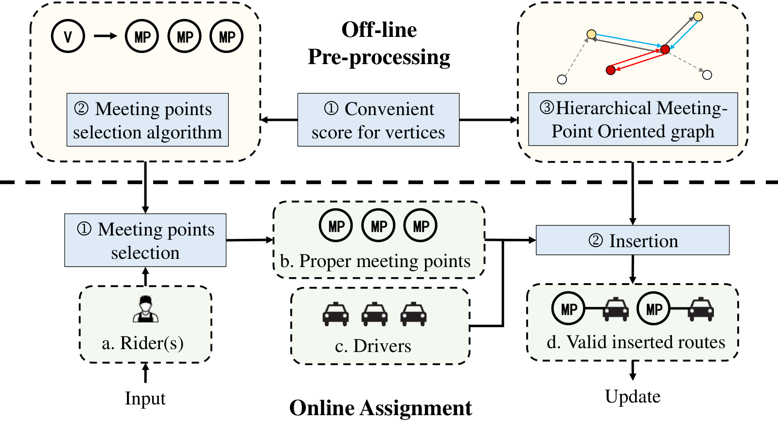
During the online assignment, requests arrive and are assigned one-by-one. Given a new request , we first select meeting points (MP) according to its source and destination locations. Then we iteratively insert each pair of MPs into each driver . In our work, we adapt the insertion algorithm with time complexity for MP insertion (Tong et al. 2018). If there exists valid insertion(s), we choose the one with the minimal unified cost; otherwise, we reject .
Compared with traditional ridesharing problem, we need to select MPs and accelerate related computations. Our work conducts off-line pre-processing to improve the efficiency and effectiveness of online assignment. we first propose a method to evaluate the convenience of each vertex, which bases on statistics of shortest path queries to meet the demand of MPs and -skip cover. MP candidates are selected for each vertex in Section 5, which greatly shrink search space with time complexity during online assignment. In addition, we design a structure, namely hierarchical meeting-point oriented graph (HMPO graph), to rank vertices for effective assignments in Section 6. -skip cover is embedded for efficiency. Based on it, we further devise a new insertion algorithm in Section 7, namely SMDB, which prunes candidate MPs and drivers during the insertion phase.
5. Select Meeting Point Candidates
After Stiglic et al. (Stiglic et al. 2015) introduced the concept of “meeting points” (MP) to provide flexible pick-up and drop-off points for riders, many researchers aim to find an effective solution for ridesharing with MPs (Stiglic et al. 2015; Czioska et al. 2017). In this paper, we pre-select a set of vertices as candidates to serve their nearby vertices.
In this section, we first introduce the motivation of selecting MP candidates. Then, we propose a heuristic algorithm, Local-Flexibility-Filter, to select them.
5.1. Meeting Point Candidates
To insert one rider into a route, traditional ridesharing only inserts 1 pair of pick-up and drop-off points. Assume that on average, one vertex has nearby vertices, which are within the acceptable distance for rider to walk to. Enumerating pick-up points and drop-off points as MPs increases the time cost by a factor of , which is unacceptable. Here, we pre-select Meeting Point Candidates for each vertex. To insert a pair of origin and destination, we can directly get their MPs, instead of searching among all their neighboors.
Definition 5.1.
(Meeting Point Candidates) Given the road network for cars and passengers , MP Candidates is a dictionary, which maps each vertex to a vertex set . For the MORP problem, we only select MPs for a vertex from its MP candidates, that is, and .
5.2. Meeting Point Candidate Selection
MP candidates should easily get to and conveniently reach other vertices. We introduce our Local-Flexibility-Filter algorithm to find the candidate sets in two phases.
Vertices convenient for drivers. The first phase aims to find the vertices which are convenient for drivers, thus boosting transportation efficiency. As the example shown in Figure 2, MPs and -skip cover have similar preferences. We quantify the convenience from the statistic of shortest path queries, named equivalent in/out cost for each vertex. If a vertex is inserted into a route between and , the and indicates the average cost from to and from to , respectively.
As riders are usually assigned to nearby drivers, shortest path queries between a vertex and its surrounding vertices will indicate its convenience. For each source vertex , we directly select its nearest vertices on the car graph as reference vertices . Intuitively, we define the equivalent out cost of as the average distance towards its reference vertices:
Similarly, for , we reverse the graph and select its nearest inward neighboors . indicates the average cost of reaching from other vertices. Here, depends on the density of a road network and the speed of drivers.
Vertices convenient for riders. The second phase takes the walking convenience into account. For each vertex , we select vertices no farther than a maximum walking distance . For each reachable vertex , we calculate a serving-cost score combining both walking distance and the equivalent in/out costs as , where and are the weight factors for driving and walking cost defined in MORP. Especially, each vertex has the SCS score for itself: .
Filtering of MP candidates. We want a small candidate set for pruning effectiveness, while only good MPs are retained. A vertex with a low average cost to serve a rider (low ) does not need alternatives. But a vertex with high needs more choices to find a good MP.
Here, for a vertex , we prune all its candidates with a score higher than . is a user-specified threshold. We also set an upper bound for the number of candidates of each vertex.
Now, we have the MP candidate set for each vertex. Once a request arrives, we find the candidate MPs only in the MP candidate sets of its source and destination.
We show an selection algorithm with detailed analysis in Appendix C.
6. Hierarchical Meeting-Point Oriented Graph
With MPs, assigned routes can be concentrated on the convenient vertices, where inconvenient ones can be replaced by nearby MPs. In this section, we first validate this assumption by analyzing the real-world data. Then we rank the vertices and design a Hierarchical Meeting-Point Oriented graph (HMPO graph). To be more specific, we 1) find defective vertices and guide us to assign riders through convenient vertices for effectiveness; and 2) further define core vertices, which form a -skip cover and reduce additional computing costs.
6.1. Graph Analysis for Meeting Point
Take the road network of New York City on Open Street Map (OSM) (OSM 2022) as an example, which contains 58189 vertices and 122337 edges. In this real-world road network, some vertices are more “convenient” than the others, which have larger traffic flows and lower transition costs. Based on this intuition, we evaluate the original road graph and vertex-flexibility with methods in Section 5. Based on the result in Section 5, vertices can be ranked by as an indication of convenience. We find that for more than 70% vertices, each of their MP candidates has at least one vertex among the 20% most convenience vertices. According to this observation, convenient vertices would be more frequently used for ridesharing with MPs compared without MPs. On the other hand, some vertices are inconvenient to drive in and out for drivers, while MPs can be their convenient alternatives. This motivates us to build a hierarchical graph, which gives an indication for effective assignment and boosts the queries on convenient vertices.
Formally, we introduce Hierarchical Meeting-Point Oriented Graph (HMPO Graph), which gives the hierarchical order over the vertex set and has 3 levels of vertices:
- •
Core vertices . They are used as MPs frequently.
- •
Defective vertices . They are inconvenient to access.
- •
Sub-level vertices . The remaining vertices are classified as sub-level vertices.
The three sets of vertices form a partition of all vertices in and , that is, and . We introduce an example below, which will be used to show the main steps of our algorithms to build a HMPO graph in this section.


6.2. Defective Vertices
Defective vertices are inconvenient vertices for vehicles to access and will be eliminated. These defective vertices are not welcomed in traditional ridesharing either, but only with meeting points, removing them is feasible as we can serve riders with MPs. However, vertex removal also induces additional travel cost. We use a heuristic method to select and remove these vertices and improve the assignment effectiveness.
Vertex removing cost. Removing a vertex from a traditional graph leads to 2 kinds of additional costs for transportation: (i) the detour cost. If a query finds a path containing , removing means that we need to find a new path without passing . The new path is usually longer than the original one and results in a detour; (ii) the inaccessibility cost, which is from queries with as origins or destinations. No path will exist after removing .
With prepared MP candidates for each vertex in , the walking cost is checked directly without query on . Thus, for assigment, shortest path queries are only on the graph , which is affected by vertex removing.
With MPs, the inaccessibility cost of removing vertices can decrease from to a limited mixture of walking and driving costs. We propose a heuristic algorithm called Defective Vertices Selection Algorithm (DVS algorithm for short) to remove the defective vertices without error from the detour cost and maintain its accessibility in the meantime. As the vertices with larger equivalent in/out cost and are harder to reach and leave, we try to remove defective vertices in decreasing order of . For each vertex, we first check its MP candidates to ensure that at least one candidate is not defective and the vertex is accessible. Then, we search the shortest path queries passing it with a bounded search space. If there is no detour cost, we mark it as defective vertex.
We show the detail of DVS algorithm with time complexity in Appendix D and an example in Appendix E. In addition, we propose two lemmas about the removing cost of defective vertices.
Lemma 6.2.
Removing all vertices selected by the DVS algorithm from with their edges leads to no detour cost.
Proof.
For details, please refer to Appendix F. ∎
Lemma 6.3.
is accessible after removing vertices selected by the DVS algorithm from with MPs.
Proof.
For details, please refer to Appendix G. ∎
| ID | ||||||
|---|---|---|---|---|---|---|
| 5.33 | 4.67 | 5.33 | 5 | 6.67 | ||
| 5.33 | 3.67 | 5.67 | 6.33 | 6.33 | ||
6.3. Core Vertices
Some convenient vertices take over the major traffic flow of a city network, such as the vertices along the highways. People in nearby places usually drive to the highway and go along it, then finally turn to small road for the destination. By assigning more route segments along highways, drivers can finish requests fast along highways in most time. With MPs, we can efficiently organize more routes along highways. Thus, these fast and request-concentrated vertices are more frequently used in solving the MORP problem. Finding such a group of convenient vertices and optimizing their related operations are pretty beneficial.
In this subsection, we select core vertices as a backbone of the whole graph. As shown in Figure 2, -skip cover (Tao et al. 2011) is a skeleton vertex set, which coincides with our demand on finding convenient vertices and accelerating their related computations. Thus, we define the Core Vertices Selection Problem to find core vertices, which have a good coverage of MP with embedded -skip cover. We first formulate the coverage of MP as an integer linear program, which can be solved with constant approximation ratio. Then, using an evaluational cost from the first step, we further complement its output and make it a -skip cover as well.
First, we define the Core Vertices Selection Problem:
Definition 6.4.
Given the union of vertices and car graph with its selected defective vertices , the Core Vertices Selection Problem is to find a set of core vertices with the minimum size , such that
(i) is a -skip cover of the updated graph with and adjacent edges removed from .
(ii) Proportion factor of vertices in passenger vertex set has at least one vertex as its MP candidate.
For attribute (i), the concept of the -skip cover is introduced in Section 2. Both of (Tao et al. 2011; Funke et al. 2014) tend to keep the vertices that are components of more shortest paths and remove the ones that belong to fewer shortest paths. They simply rank their vertices according to the degree, which is pretty coarse as road network has very low vertex degree. Instead, we use a cost which is evaluated from the internal connections between vertices for ranking, aiming at comparing vertex importances more quantitatively. Attributes (ii) assures that most of the requests can be assigned with core vertices as MPs. So the optimization for core vertices can benefit more assignments. If a set of core vertices is valid to represent the graph skeleton, the smaller its size is, the more efficient its inner operations are after further preprocessing. So, we want to find a which satisfies attribute (i) (ii) with minimal size.
Now, to satisfy the attribute (ii), we can formulate an equivalent interger linear program. The detailed mapping steps include: (i) constructing candidate serving set to indicate the set of servable vertices for each vertex , that is, for any pair of vertex , iff . As an inverse-function relationship of , we can convert the MP candidate set by scanning each vertex and for each , add to . This process is linear; (ii) the universe is defined to be the set of all the passenger-accessible-vertices ; (iii) find the smallest sub-collection of vertices that the union of their serving sets covers at least of the universe, that is, .
Mathematically, we have the following integer linear program (ILP):
| (2) | |||||
where iff vertex is chosen to serve its candidate serving set . The binary variable iff vertex is not served by any selected vertex.
The partial set cover problem is an NPC problem. Luckily, in our setting, each element (vertex) is in at most candidate serving sets as the times of adding a vertex to some equals to the number of ’s MP candidates . Such a case is called a low-frequency system. There exists a solution to approximate the optimum within a factor using LP relaxation in polynomial time (Gandhi et al. 2004). In detail, the corresponding LP relaxation can be derived by substituting the constraints by and by . Then the problem is transferred to a linear Program . After deriving the dual LP of it, (Gandhi et al. 2004) iteratively chooses each set to be the highest cost set and obtains a feasible cover with the primal-dual stage. This step generates a cost for each set. Intuitively, in our setting, this cost can be treated as how bad the “quantity” each vertex with its serving set to be included in the final output. The higher its value, the worse a vertex is. Finally, it chooses the solution with minimum cost.
However, to guarantee attribute (i) simultaneously, we cannot apply this algorithm directly to our problem. Both of the two attributes require the set of chosen vertices to have a good “coverage” of other vertices, that is, each of them can serve many nearby vertices. Motivated by this observation, we first use our equivalent in/out cost as a coarse estimation in the solution of (Gandhi et al. 2004). Then we use the of (Gandhi et al. 2004) as the ranking for -skip cover completion. For the detail of our CVS algorithm and complexity analysis, please refer to Appendix H.
We show that the size of is bounded with the following lemma and present an example below.
Lemma 6.5.
Assume that we have vertices in total, with set as optimal solution for the attribute (ii), the upper bound of the size of core vertex set is .
Proof.
For details, please refer to Appendix I. ∎
Example 6.6.
Let us continue using the setting in Example 6.1. After selecting and to , we select the core vertices among the rest of vertices. We set to guarantee that no fewer than vertices are covered. and the result of partial set cover are shown in Table 2. The final cover is with cost 2. To maintain a -skip cover, we initialize and iteratively check each vertex . As none of these removals violates the 2-skip cover, both of them are removed from . Removing or violates attribute (ii) and we finally output .
| ID | ||||
|---|---|---|---|---|
| Partial set cover | ||||
| Cost |
Finally, as , , and is a partition of , .
6.4. Construction of HMPO colorred Graph and Fast Query
After obtaining the three levels of vertices, we use them to construct the hierarchical graph . In this subsection, we first concentrate on the formulation of edge . Then, we show that how to compute shortest path queries fast on .
HMPO graph construction. First, for the defective vertices, we “discard” them so there is no edge for drivers to come nor leave them. We get an updated car graph by removing and its adjacent vertices from
Recall that is a -skip cover of . Based on that, all the shortest distance queries can be answered by efficiently.
Core vertices serve as the skeleton of the original road network. Borrowing the definition in the previous work (Tao et al. 2011), for each , one can find its -skip neighbors and build super-edges, leading to a new graph for fast query. To be more specific, one can construct a graph , which has 2 vertex sets and and 3 edge sets , , and . Any query result between these core vertices on the new graph is the same as that on the original graph. Query start from or aim at sub-level vertices can be answered by temporally extending the graph with super-edges between sub-level vertex and its nearby core vertices.
Here we summarize the construction steps. (1) Instead of the -skip neighbors of , , we can find a superset of efficiently according to (Tao et al. 2011). (2) We build super-edge, which is weighted by the shortest path distance between two vertices, from to each . Add these super-edges between core vertices to . (3) For , we find its on and on the reversed graph. The super-edges built to are stored into edge set , each represents a path from a sub-level vertex to a core vertex. Similarly, the super-edges built to are stored into edge set for core-to-sub-level vertex pairs. (4) In the middle of finding for each , every sharing a shortest path with without core vertex generates a sub-to-sub level super-edge, added to .
Fast queries. We can calculate the exact -shortest path using the three edge sets (Tao et al. 2011). Consider the following cases: (i) . We simply return the query result on graph ; (ii) . First we check the super-edges of in . If can reach directly, return the weight of super-edge. Otherwise, follow the general cases in (iii, iv); (iii) . We need an additional step to add with its super-edges into ; (iv) . Add with its super-edges into and return the query result. Its correctness has been proved. For details, please refer to (Tao et al. 2011).
In summary, our final output for HMPO graph is consists of: , which forms the graph for query together with super-edges ; , of which each vertex is added to with edge sets temporally for query; , which is only called at the route planning stage with . and .

Example 6.7.
Following the setting in Example 6.1, we construct the in Figure 5. are marked in white and their edges are removed. are marked in dark red. Sub-level vertices are marked in light yellow. Two core-to-core edges between them are added to and marked in red. Two edges from to and are added to and marked in grey. Two edges from and to are added to and marked in blue.
7. HMPO Graph Based Insertor

With the HMPO Graph, we introduce a new algorithm to boost the insertion phase for the solution of MORP problem.
Requests are served one-by-one, where the MP candidates of their origins and destinations are inserted into drivers’ routes. With limited walking distance, the MP candidates for each are close to each other. One interesting problem is, if we fail to insert a candidate , do the rest help? To answer it, we define a new distance correlation, which bounds the time saving of switching to any vertex in . If deducting the saving still cannot meet the time limitation, we can safely prune the whole set. However, to derive it on the traditional graph, we need all the distances from sources even though vertices in are close to each other. Fortunately, we find that based on the -skip structure in our hierarchical graph, an upper bound can be derived effectively. As shown in Figure 2, -skip cover “cuts off” the shortest paths using the core vertices, which can be used as anchors to compare the difference between the paths from the same source to a pair of vertices. Most of the related works only use k-skip cover for faster query and vertex clustering (Cheng et al. 2017). To the best of our knowledge, this is the first paper to explore this property of k-skip cover graph for task assignment.
We demonstrate an example through this section in Figure 6. The network and edge weights are consistent with Figure 2(a), where red vertices belong to core vertices and yellow ones belong to sub-level vertices. In Figure 6(b), a rider is waiting to be picked up at origin and a driver is at . The MP candidates for are . We want to know that if driver cannot reach MP / in time, can we prune the other MP.
In the following subsections, we first extract the important distance correlations in subsection 7.1, then devise an effective algorithm SMDB for MORP problem in subsection 7.2.
7.1. Maximum Difference for Reaching Distances
Insertion for MPs induces many shortest path queries, which are from the same source to closely-located MPs. Here, we bound the distance differences between these queries. We first give related definitions for the bound. Given a vertex and its MP candidates , we have (i) one checker vertex , and (ii) the distance bound, named set maximum difference (). We show that after computing the query of one long path from a vertex to checker , (i.e., ), the distance from to any other candidate vertices is no shorter than .
In this subsection, we first introduce the above concepts. Then, as any shortest path is split by -skip cover , we can quickly derive the bound locally, where only the subgraph formed by surrounding is needed.
First, we define maximum difference between two vertices as a general distance correlation as follows:
Definition 7.1.
(Maximum Difference) Given a graph , for each pair of vertices , the maximum difference for and is:
In general, starting from any source , the largest difference between distances to reach two given vertices is denoted as their .
When we insert a set of MP candidates of source or destination into a route, it is more reasonable to use a set-based relationship for maximum difference rather than pairwise . To be more specific, for the MP candidates of vertex , by defining a checker vertex , we want to know the Maximum Differences between checker and all the vertices in the candidate set. The upper bound of these s is defined as set maximum difference (). That is,
In the following part, we show that for a modified with narrower source vertices, which are not sub-level vertices that have super-edges to , the -skip structure can help us get in time. Mathematically, we define
and
| (3) |
where and are super-edge sets in Section 6.4.
With a -skip cover , any shortest paths of length ended at a vertex must reach its surrounding . Our core vertices , also a -skip cover, further builds super edges between and these surrounding . As shown in Figure 6(c), any paths ended at and need reach , and first. They are also the only 4 vertices having super edges with and in the HMPO graph, e.g., Figure 6(d). We check super edges and get the surrounding for each vertex in an MP candidate set and define their union as . In Figure 6, . As vertices in are close to each other, is a small set.
Note that the distance from any to any is already recorded in HMPO graph, which does not need to compute. We denote its cost as . By fixing a vertex as checker vertex, we can compute the following Local Maximum Difference quickly:
Now, we have the following Lemma:
Lemma 7.2.
If we use as the checker vertex, the Local Maximum Difference is a valid Set Maximum Difference . Mathematically, if a vertex has no super-edge towards any , then .
Proof.
We prove it by contradiction. Given a vertex and its with outputs and , assume that has no super-edges in to , which satisfies . We denote the last core vertex in the path from to as . Here we have
As is the last core vertex along the path, must be a -skip neighbors of . Thus, we have:
Contradiction. The original lemma is proved. ∎
For example, in Figure 6(f), if we choose and check vertex, we can calculate and . So when or . After we compute the cost from to as , we want to bound the cost from to (i.e., ). In Figure 6(g), its last passed core vertex is . we have .
Now we can efficiently find given a checker. Here, we show the detail in our HMPO Graph-based Maximum Difference Generator (HMDG), which finds the for each that minimize when calculating .
Algorithm sketch Lines 3-8 collect all the cost from vertices to vertices . As , if , we check the its super edges from core to core vertices. The costs are stored in the form of dictionary ; if , we check its super edges from sub to core vertices instead.
Secondly, we initialize as a dictionary, which can be further used to choose the checker with minimal . Instead of fixing checker and calculating corresponding , for each , we find the vertex which has minimal in line 11, that is, among vertices in , is the closest destination for . If we use as checker, the is the maximal of , which should be minimized. Lines 12-14 enumerate and update the if a higher maximum difference is found, that is, . Finally, saves the required for each checker. We find the minimal value of with its key and return and .
So our algorithm finds with such that: (i) for any source from nearby core vertices, , ; (ii) is chosen among to minimize .
Time Complexity. The time costs of Lines 2 and 3 are . There are iterations in lines 4-8 and each iteration costs , where is the number of super edges a vertex has on average. Line 9 costs time. Line 11 costs to find the minimum value and lines 12-14 form iterations taking time in each iteration. For the size of , we borrow the definition from (Tao et al. 2011), where is the average number of k-hop neighbors of the vertices in . Thus, there are iterations in lines 10-14. Their total time complexity is . Line 15 cost to find the minimum. So the total time complexity of the big loop in lines 1-15 is and grows linearly with , where both and depend on the structure of the road network instead of the size.
Note that, though we only discuss the distance relationships from the same source to different destinations, similar property still hold for queries from different sources to the same destination. We further emphasize that such a relationship is not only applicable for meeting points, but a property of -skip cover. It is useful for many crowdsourcing scenarios, which have shortest path queries with close sources and destinations.
7.2. SMD-Boost Algorithm
We use to boost insertion in this subsection.
Recall that whenever we try to insert a request into a route, the rider should be picked up no later than . Considering that we try to insert one pick-up into a fixed position of route. If we use as the MP, it is not insertable if the time to pick up rider at , denoted as here, is later than . The worker needs to pick up rider at least earlier. In the last subsection, we find the maximum time saving for each checker, . If of is smaller than , no matter which MP of is used for insertion, we cannot pick up the request by . In such case, there is no need to try other MPs for insertion with the help of .
We illustrate our algorithm SMDBoost for the insertion phase in Algorithm 2. Note that we add one more set for pruning, dead vertices . It means that no driver with current location can serve this rider. We initialize for each new request. Assume that we try to insert rider into the route of driver . First, if , we can prune driver . Otherwise, we derive arriving time for each route vertex according to (Tong et al. 2018). In line 4, all the sub-level vertices which have super-edges towards are collected into a set , which covers vertices that cannot be pruned. This is because that distances between these vertices and an MP can be arbitrarily short through super-edges in and not follow the definition of in Equation 3.
Pruning strategy in lines 5-12 finds the largest index to insert any pick-up in . We initialize . Then we check each vertex in order. As the distances from vertices in to some MPs in can be arbitrarily short, if , it is possible to insert rider after . In this case, we continue to check the next insertion position in line 8. For each vertex , it can be viewed as a source for subject to . So if , according to Lemma.7.2, inserting any MP after misses the deadline . Insertion position can only be smaller than index of denoted as , that is, . A special case is that if inserting after the driver’s current location cannot catch , driver and all the other drivers at currently can not serve . So we add into for future pruning.
After the checking phase, we insert without checking indexes after for the pick-up point. The base algorithm adapts the linear insertion algorithm (Tong et al. 2018) for MPs.
Time Complexity. Line 3 is a linear operation according to (Tong et al. 2018). Line 4 costs . There is an loop in lines 5-12. All other lines from 1 to 12 cost . As the algorithm in line 13 is linear, the total time complexity is .
Lemma 7.3.
Pruning Algorithm 2 has no performance loss.
Proof.
For details, please refer to Appendix J. ∎
For example, in Figure 6(g), assume that rider needs to be picked up in 10 time steps. If the shortest path from to is 12 time steps, as is 1, the shortest time to reach any other MP candidates is bounded by . We can stop checking other MP candidate(s) (). Any other worker at currently cannot serve . is marked as a dead vertex and added to .
8. Experimental Study
8.1. Experimental Methodology
Data set. We use both real and synthetic data to test our HMPO Graph-Based solution. Specifically, for the real data, we use a public data set NYC (NYC 2021). It is collected from two types of taxis (yellow and green) in New York City, USA. We use all the request data on December 30th to simulate the ridesharing requests in our experiments. Each taxi request in NYC contains the latitudes/longitudes of its source/destination locations, its starting timestamp, and its capacity. We can generate a ridesharing request and initialize its locations, release time, and capacity correspondingly.
In addition, we derive the distribution of requests of all the NYC requests in December and generate 5 synthetic datasets (Syn) with the size of requests as 100k, 200k, 400k, 800k, and 1000k. We extract the road network of NYC from Geofabrik (geo 2022). It includes the labels of roads for both driving and walking. We clean it into the directed car graph and passenger graph according to road labels. The road network is widely used in existing ridesharing studies (Tong et al. 2018).
The settings of our dataset are summarized in Table 3.
| Parameters | Settings |
|---|---|
| Number of vertices of NYC | 57030 |
| Number of edges of NYC | 122337 |
| Number of valid requests of NYC | 277410 |
Implementation. We follow the common settings for simulating ridesharing applications in (Asghari et al. 2016; Huang et al. 2014; Tong et al. 2018). While building the graph for road network, the weights of edges are set to their time cost (divide the road length on Geofabric by the velocity of its road type). The walking speed is set to 3.6km/h, while the driving speed varies according to the road type in OSM, i.e., 60% of the maximum legal speed limit in their cities (Spe 2022). For each request, we map its source and destination to the closest vertex in the road network. The initial location of each driver is randomly chosen.
8.2. Setting Default Values for Parameters
| Parameters | Settings |
|---|---|
| Deadline Coefficient | 0.1, 0.2, 0.3, 0.4, 0.5 |
| Capacity | 2, 3, 4, 7, 10 |
| Driving Distance Weight | 1 |
| Walking Distance Weight | 0.5, 1, 1.5, 2 |
| Penalty | 3, 5, 10, 15, 30 |
| Number of drivers | 5k, 10k, 20k, 30k, 40k |
| Number of requests | 100k, 200k, 400k, 800k, 1000K |
Table 4 summarizes the major parameter settings for our experiments, where default values are in bold font. Other hyperparameters are discussed in Appendix1 K with extensive experiments.
Note that for a mix mode where some riders are not willing to walk, our algorithm SMDB can directly handle it by manipulating its input. Instead of generating meeting point candidates according to Section 5, we restrict the candidates as source for pick-up point and destination for drop-off point, where the walking distance is 0. The candidates are fed into SMDB, which still works regardless of the number of candidates.
The experiments are conducted on a server with Intel(R) Xeon(R) E5 2.30GHz processors with hyper-threading enabled and 128 GB memory. The simulation implementation is single-threaded, and the total running time is limited to 14 hours for NYC. In reality, a real-time solution should stop before its time limit (24 hours for us) (Huang et al. 2014; Tong et al. 2018). All the algorithms are implemented in Java 11. We first preprocess our road network according to Section 6. The modified vertices and weighted edges can be loaded directly for route planning. We boost the shortest distance and path queries with an LRU cache according to the previous studies (Huang et al. 2014; Tong et al. 2018).
Compared Algorithms. We compare SMDB with the state-of-the-art algorithms for route planning of ride-sharing.
- •
GreedyDP (Tong et al. 2018). It uses a greedy strategy for route planning without MPs. Each request is assigned to the feasible new route with minimum increased cost.
- •
Kinetic Tree (KT). For each driver, it saves all the possible routes for the assigned request using a structure called Kinetic Tree. The new request is inserted by traversing and updating the tree, which is more local optimal but slower compared with GreedyDP.
- •
BasicMP. It is an extension from GreedyDP by adapting MPs to solve the MORP problem.
- •
First Serve (FS). A variant of BasicMP, where each request is directly assigned to the first driver who can serve it.
- •
HSRP. It uses the HMPO Graph to improve the effectiveness of BasicMP without pruning.
Metrics. All the algorithms are evaluated in terms of total unified cost, served requests and response time (average waiting time to arrange a request, resp. time for short), which are widely used as metrics in large-scale online ride-sharing proposals (Huang et al. 2014; Ma et al. 2013; Tong et al. 2018).
8.3. Experimental Results
In this subsection, we present the experimental results.
Impact of Number of Drivers . The first column of Figure 7 presents the results with different numbers of drivers in NYC. Compared with GreedyDP, BasicMP outperforms it in terms of the number of served requests by 6.6% to 12.7% with the help of MPs, while SMDB and HSRP outperforms it by 21.4% to 29.9%. More requests are served with more drivers, results in a decrease of unified costs and an increase in the served rates of all the algorithms. BasicMP decreases the cost by 2.7% to 13.2% and SMDB decreases it by 4.5% to 32.7%. GreedyDP and FS run the fastest, where GreedyDP does not use MPs and FS assigns each request to the first feasible worker suboptimally. SMDB runs faster than other local-optimal MP-based methods ( HSRP and BasicMP) with a resp. time .
Impact of Capacity of Drivers . The second column of Figure 7 presents the effect of the capacities of drivers. BasicMP serves 8.6% to 12.2% more requests than GreedyDP with 5.1% to 9.2% less cost. SMDB outperforms other algorithms on both serving rate, 27.3% to 33.1% higher than GreedyDP, and unified cost, 13.0% to 20.5% less than GreedyDP. With a larger capacity, all the algorithms serve more requests with lower costs. However, the improvement with capacity from 4 to 10 is not as significant as from 2 to 4. The reason is that the extra spaces are mostly wasted. GreedyDP and FS still runs faster but serve fewer requests. SMDB costs less time than BasicMP and HSRP. KT is much slower than other methods but serves the fewest requests.
Impact of Deadline Coefficient . The third column of Figure 7 shows the results of varying the deadline coefficient . With larger , all the algorithms serve more requests with a lower unified cost. SMDB still serves more requests with lower cost, which outperforms GreedyDP by serving 26.6% to 30.3% more requests than GreedyDP and decreasing its cost by 9.8% to 18.7%. With meeting points, BasicMP increases the number of served requests by 8.0% to 12.6% and decreases the cost by 3.4% to 9.2% compared with GreedyDP. With a larger deadline coefficient , they find more feasible routes and serve more requests. KT builds tree to record all the possible routes for each driver, which even fails to finish with . Time cost increases with larger as each request can find more feasible candidate routes. GreedyDP and FS still run the fastest and SMDB is faster than BasicMP and HSRP.
Impact of Number of Requests . The fourth column of Figure 7 displays the results on different sizes of synthetic requests. The datasets are generated based on the distribution of all the NYC requests in December. We increase the number of requests from 10k to 100k to test the extreme case that drivers are fully busy, i.e., the number of served requests does not increase with 100k arrival requests compared with 80k requests for all the algorithms.
When drivers are not fully busy with requests fewer than 80k, all the algorithms serve more requests with a lower unified cost as the increases. Comparing with each other, SMDB serves 7.3% to 28.4% more requests than GreedyDP and decreasing its cost by 10.6% to 21.8%. BasicMP works weaker that increases the number of served requests by 3.3% to 10.8% and decreases the cost by 5.0% to 14.8% compared with GreedyDP. Response time of KT drops quickly with more requests while it rejects more requests. SMDB has a closer response time compared with GreedyDP and FS with increasing , where HSRP and BasicMP are the slowest methods.
Summary of Results.
- •
Our SMDB algorithm can serve 7.3% to 33.1% more requests than the state-of-art algorithm (Tong et al. 2018). The unified cost is decreased by 4.5% to 32.7%. These results validate the effectiveness of our algorithm in large scale datasets.
- •
With MPs, BasicMP, HSRP, and SMDB outperform GreedyDP and KT. Suboptimal MP-based First Serve method also has competitive performance compared to GreedyDP. SMDB potentially arranges more requests on the highway and prunes candidates, which uses less time to serve more requests than BasicMP and HSRP. On the real-world dataset, SMDB can save 11% to 24% time compared with HSRP. On the synthetic dataset where a large amount of requests is test, SMDB saves more time (up to 31% compared with HSRP) given more requests, which is important to handle heavy traffic cases. With a response time lower than 0.2 seconds, SMDB is acceptable to be used as a real-time solution for ridesharing tasks.
9. Conclusion
In this paper, we propose the MORP problem, which utilizes meeting points for better ride-sharing route planning. We formulate a modified objective function to cover the cost of walking. We prove that the MORP problem is NP-hard and there is no polynomial-time algorithm with a constant competitive ratio for it. To cut the search space of meeting points for fast assignemnts, we devise an algorithm to prepare meeting point candidates for each vertex. Besides, we construct an HMPO graph with hierarchical order on vertices for fast route planning, which takes the advantage of flexibility from meeting points to improve efficacy. Based on it, we propose SMDB algorithm to solve MORP problem effectively and efficiently. Extensive experiments on real and synthetic datasets show that our proposed solution outperforms baseline and the state-of-the-art algorithms for traditional ridesharing in effectiveness greatly without losing too much efficiency. Our paper is provided as a comprehensive theoretical reference for optimizing route planning with meeting points in ridesharing.
Acknowledgements.
Peng Cheng’s work is partially supported by the National Natural Science Foundation of China under Grant No. 62102149, Shanghai Pujiang Program 19PJ1403300 and Open Foundation of Key Laboratory of Transport Industry of Big Data Application Technologies for Comprehensive Transport. Libin Zheng is supported by the National Natural Science Foundation of China No. 62102463, the Natural Science Foundation of Guangdong Province of China No. 2022A1515011135 and the Fundamental Research Funds for the Central Universities, Sun Yat-sen University No. 22qntd1101. Wenjie Zhang’s work is partially supported by the ARC Future Fellowship FT210100303. Corresponding author: Peng Cheng.References
- (1)
- Exp (2019) 2019. [Online] Express Pool. https://www.uber.com/us/en/ride/express-pool/.
- Ube (2019) 2019. [Online] Uber Express Just like a Bus. https://gizmodo.com/i-tried-uber-s-new-pool-express-service-and-honestly-j-1823190462.
- NYC (2021) 2021. [Online] TLC Trip Record Data. https://www1.nyc.gov/site/tlc/about/tlc-trip-record-data.page.
- did (2022) 2022. [Online] Didi Chuxing. http://www.didichuxing.com/.
- geo (2022) 2022. [Online] Geofabrik. https://download.geofabrik.de/.
- OSM (2022) 2022. [Online] Open Street Map. https://www.openstreetmap.org/.
- Spe (2022) 2022. [Online] Speed limits in the United States – Wikipedia. https://en.wikipedia.org/wiki/Speed_limits_in_the_United_States.
- Alonso-Mora et al. (2017) Javier Alonso-Mora, Samitha Samaranayake, Alex Wallar, Emilio Frazzoli, and Daniela Rus. 2017. On-demand high-capacity ride-sharing via dynamic trip-vehicle assignment. PNAS (2017).
- Asghari et al. (2016) Mohammad Asghari, Dingxiong Deng, Cyrus Shahabi, Ugur Demiryurek, and Yaguang Li. 2016. Price-aware real-time ride-sharing at scale: an auction-based approach. In SIGSPATIAL. ACM.
- Asghari and Shahabi (2017) Mohammad Asghari and Cyrus Shahabi. 2017. An On-line Truthful and Individually Rational Pricing Mechanism for Ride-sharing. In SIGSPATIAL. ACM.
- Cheng et al. (2017) Peng Cheng, Hao Xin, and Lei Chen. 2017. Utility-Aware Ridesharing on Road Networks. In SIGMOD. ACM.
- Cici et al. (2015) Blerim Cici, Athina Markopoulou, and Nikolaos Laoutaris. 2015. Designing an on-line ride-sharing system. In SIGSPATIAL. ACM.
- Czioska et al. (2017) Paul Czioska, Dirk C Mattfeld, and Monika Sester. 2017. GIS-based identification and assessment of suitable meeting point locations for ride-sharing. Transportation Research Procedia (2017).
- d’Orey et al. (2012) Pedro M. d’Orey, Ricardo Fernandes, and Michel Ferreira. 2012. Empirical evaluation of a dynamic and distributed taxi-sharing system. In ITSC. IEEE.
- Eser et al. (2018) Elif Eser, Julien Monteil, and Andrea Simonetto. 2018. On the tracking of dynamical optimal meeting points. IFAC-PapersOnLine (2018).
- Feuerstein and Stougie (2001) Esteban Feuerstein and Leen Stougie. 2001. On-line single-server dial-a-ride problems. Theor. Comput. Sci. (2001).
- Funke et al. (2014) Stefan Funke, André Nusser, and Sabine Storandt. 2014. On k-Path Covers and their Applications. PVLDB (2014).
- Gandhi et al. (2004) Rajiv Gandhi, Samir Khuller, and Aravind Srinivasan. 2004. Approximation algorithms for partial covering problems. J. Algorithms (2004).
- Gschwind and Irnich (2015) Timo Gschwind and Stefan Irnich. 2015. Effective Handling of Dynamic Time Windows and Its Application to Solving the Dial-a-Ride Problem. Transportation Science (2015).
- Gupta et al. (2010) Anupam Gupta, Mohammad Taghi Hajiaghayi, Viswanath Nagarajan, and R. Ravi. 2010. Dial a Ride from k-forest. ACM Trans. Algorithms (2010).
- Herbawi and Weber (2012) Wesam Herbawi and Michael Weber. 2012. A genetic and insertion heuristic algorithm for solving the dynamic ridematching problem with time windows. In GECCO. ACM.
- Ho et al. (2018) Sin C Ho, WY Szeto, Yong-Hong Kuo, Janny MY Leung, Matthew Petering, and Terence WH Tou. 2018. A survey of dial-a-ride problems: Literature review and recent developments. Transportation Research Part B: Methodological (2018).
- Huang et al. (2014) Yan Huang, Favyen Bastani, Ruoming Jin, and Xiaoyang Sean Wang. 2014. Large Scale Real-time Ridesharing with Service Guarantee on Road Networks. PVLDB (2014).
- Jaw (1984) Jang-Jei Jaw. 1984. Solving large-scale dial-a-ride vehicle routing and scheduling problems. Ph.D. Dissertation. Massachusetts Institute of Technology.
- Kleiner et al. (2011) Alexander Kleiner, Bernhard Nebel, and Vittorio A. Ziparo. 2011. A Mechanism for Dynamic Ride Sharing Based on Parallel Auctions. In IJCAI.
- Ma et al. (2013) Shuo Ma, Yu Zheng, and Ouri Wolfson. 2013. T-share: A large-scale dynamic taxi ridesharing service. In ICDE. IEEE.
- Ma et al. (2015) Shuo Ma, Yu Zheng, and Ouri Wolfson. 2015. Real-Time City-Scale Taxi Ridesharing. IEEE Trans. Knowl. Data Eng. (2015).
- Ota et al. (2017) Masayo Ota, Huy T. Vo, Cláudio T. Silva, and Juliana Freire. 2017. STaRS: Simulating Taxi Ride Sharing at Scale. IEEE Trans. Big Data (2017).
- Rubinstein et al. (2012) Zachary B. Rubinstein, Stephen F. Smith, and Laura Barbulescu. 2012. Incremental Management of Oversubscribed Vehicle Schedules in Dynamic Dial-A-Ride Problems. In AAAI.
- Santos and Xavier (2013) Douglas Oliveira Santos and Eduardo Candido Xavier. 2013. Dynamic Taxi and Ridesharing: A Framework and Heuristics for the Optimization Problem. In IJCAI.
- Stiglic et al. (2015) Mitja Stiglic, Niels Agatz, Martin Savelsbergh, and Mirko Gradisar. 2015. The benefits of meeting points in ride-sharing systems. Transportation Research Part B: Methodological (2015).
- SUMC (2018) SUMC. 2018. What is shared-use mobility? https://goo.gl/3Jw6z7.
- Tao et al. (2011) Yufei Tao, Cheng Sheng, and Jian Pei. 2011. On k-skip shortest paths. In SIGMOD. ACM.
- Thangaraj et al. (2017) Raja Subramaniam Thangaraj, Koyel Mukherjee, Gurulingesh Raravi, Asmita Metrewar, Narendra Annamaneni, and Koushik Chattopadhyay. 2017. Xhare-a-Ride: A Search Optimized Dynamic Ride Sharing System with Approximation Guarantee. In ICDE. IEEE.
- Tong et al. (2017) Yongxin Tong, Libin Wang, Zimu Zhou, Bolin Ding, Lei Chen, Jieping Ye, and Ke Xu. 2017. Flexible Online Task Assignment in Real-Time Spatial Data. PVLDB (2017).
- Tong et al. (2018) Yongxin Tong, Yuxiang Zeng, Zimu Zhou, Lei Chen, Jieping Ye, and Ke Xu. 2018. A Unified Approach to Route Planning for Shared Mobility. PVLDB (2018).
- Wilson et al. (1975) Nigel HM Wilson, RW Weissberg, BT Higonnet, and J Hauser. 1975. Advanced dial-a-ride algorithms. Technical Report.
- Wilson et al. (1976) Nigel Henry Moir Wilson, Richard Wayne Weissberg, and John Hauser. 1976. Advanced dial-a-ride algorithms research project. Technical Report.
- Yao (1977) Andrew Chi-Chih Yao. 1977. Probabilistic Computations: Toward a Unified Measure of Complexity (Extended Abstract). In FOCS. IEEE.
- Yeung et al. (2016) San Yeung, Evan Miller, and Sanjay Madria. 2016. A Flexible Real-Time Ridesharing System Considering Current Road Conditions. In MDM. IEEE.
- Zhao et al. (2018) Meng Zhao, Jiateng Yin, Shi An, Jian Wang, and Dejian Feng. 2018. Ridesharing Problem with Flexible Pickup and Delivery Locations for App-Based Transportation Service: Mathematical Modeling and Decomposition Methods. Journal of Advanced Transportation (2018).
- Zheng et al. (2018) Libin Zheng, Lei Chen, and Jieping Ye. 2018. Order Dispatch in Price-aware Ridesharing. PVLDB (2018).
Appendix A Proof of Lemma 3.6
Lemma III.1. The MORP problem is NP-hard.
Proof.
The basic route planning for ridesharing problems, which only takes the driving cost and rejection cost into account, is NP-hard (Tong et al. 2018). A reduction from it to the MORP problem can be established by setting to ban walking. So MORP problem is NP-hard. ∎
Appendix B Proof of Lemma 3.7
Lemma III.2. There is no randomized or deterministic algorithm guaranteeing constant CP for the MORP problem.
Proof.
By proving no deterministic algorithm can generate constant expected value (e.g., ) with a distribution of the input including the destinations of the requests, the previous work (Tong et al. 2018) guarantees that no randomized algorithm has a constant CP using Yao’s Principle (Yao 1977), which is also applicable for our problem. Our problem is a variant of the basic problem as stated in the proof of Lemma 3.6. Thus, no randomized or deterministic algorithm guarantees constant CP for MORP. ∎
Appendix C Local-Flexibility-Filter Algorithm
Algorithm sketch. Algo. 3 Local-Flexibility-Filter Algorithm (LFF Algorithm for short) shows the detail of our candidate selection solution. As vertices in road network have bounded number of adjacent edges (usually no more than 5), the degree of a vertex can be regarded as . We will stop after finding nearest vertices in line 5 and line 8, so there are rounds to pop vertex and relax edge. The time complexity of lines 5-8 is . The total time complexity from lines 4 to 8 is thus . We assume that given any vertex , the maximum number of vertices that can reach within on is , line 10 would have a time complexity . Line 12 costs by using a min-heap to keep top points. The lines 11-12 thus costs . Line 13 costs . The total cost from line 9 to 13 is . Because maximal number of candidates is always smaller than the number of reachable vertices, that is, , the time complexity of LFF algorithm is .
Appendix D Defective Vertices Selection Algorithm
Algorithm sketch. The pseudo code of the DVS approach is shown in Algorithm 4. The main idea of the DVS approach is to ensure that: (a) every selected defective vertex will have at least one MP candidate existing in the rest vertices (i.e., core vertices or sub-level vertices); (b) the travel cost of any two vertices in will not increase after removing the defective vertices and their related edges.
The implementation of the DVS approach (Algorithm 4) can be summarized in 3 steps:
(i) Sort in descending order of ;
(ii) Initialize each vertex as unmarked, which means that it is not required by any defective vertices as MP;
(iii) pop vertices one-by-one. For each vertex , check whether it is marked or its MP candidates are all in . If so, pop the next vertex. Otherwise, remove it from and record each vertex which has an edge with . If the edge starts from (an edge comes to ), we add into a set with the weight ; if it starts from , we add into a set with the weight . Save the sum of the largest in and out weights as . Then we remove with its adjacent edges from . For each vertex , we run the Dijstra algorithm from source until the new reached vertex costs more than . If any is accessed with cost larger than , we refuse to add into and check next one. If all vertices in have been accessed, add to and mark vertices in . and its edges are recovered if we failed to add it to .
A vertex with a large / is hard to reach and leave, thus it has a high possibility to be isolated from the city center and the main street. Removing the defective vertices will have little influence on the connectivity of the road network. We sort the vertices according to their and at the beginning of DVS, which help us remove the unimportant vertices first as they affect fewer vertices, such that a more concise HMPO graph can be achieved.
Time Complexity. We assume that each vertex has an degree, which is common in road networks. Line 1 runs in time, where . Lines 7 and 8 collect adjacent vertices in time as degree is in scale. Assume that (i) the longest length-2 path in costs ; (ii) given any vertex , the number of vertices that can reach within cost is no larger than , then the number of accessed vertices is bounded by . Thus, line 12 is a -time-complexity loop. All checking phases (lines 5, 13, 17) are implemented in hash index and cost . Loop from lines 11 to 19 and loop from lines 16 to 19 enumerate vertices. Loop from line 4 to 20 enumerates vertices. Thus, the overall time complexity is .
Appendix E Example for Algorithm D
Example E.1.
Let us continue the setting in Example 6.1. Now we want to select the defective vertices among them. We first sort the vertices and initial their labels as unmarked. Then we check all the vertices one-by-one and show their status at each round with a row in Table 5. Round 0 initializes flags as unmarked (). Round 1 pops and there is no node in . We add it to and mark its candidates as . In the table we use to suggest that is added to . Round 2 adds to and updates its unmarked candidate(s) (). Rounds 3 5 all pop marked vertices and fail to add a new vertex to . Round 6 checks the by first removing it from the graph with edges and recording its with . Running Dijkstra algorithm from results in cost and poping is rejected. We mark the failed ones as .
| Round | ||||||
|---|---|---|---|---|---|---|
Appendix F Proof of Lemma 6.2
Lemma V.1. Removing all vertices selected by the DVS algorithm from with their edges leads to no detour cost.
Proof.
Recall that if a shortest path query finds a route contains a vertex in the middle, we need to find an alternative path without after removing from graph . If the new route has higher cost, removing results in a detour cost. We define the new car graph without as . Hereby the proof is equivalent to proof , where is the shortest distance query on graph . We prove it by construction, that is, given any shortest path on from to , where , we show that there is a path from to on with the same cost.
We use to denote the removed defective vertices in order. When we remove a , any length-2 shortest path must have a same cost substitution , where , . It is satisfied according to the phase (iii) of Algorithm 4.
Then, for any path on from to , we can iteratively find each with the lowest index. Denote its previous and latter vertices as , we substitute with . In each round, the lowest index of in the new path is increasing. After at most rounds, the path has no vertex in . As each substitution does not increase the cost, the final substitution is a valid path on with cost equal to . ∎
Appendix G Proof of Lemma 6.3
Lemma V.2. is accessible after removing vertices selected by the DVS algorithm from with the help of meeting points.
Proof.
After popping each vertex in phase 3 of the DVS algorithm, we ensure that is in to guarantee that any vertex without available meeting points is still in graph . Once a request starts from or aims at , we can serve it by itself. On the other hand, if a vertex is added to , we mark its meeting point candidates so that we would not further remove these vertices from . Request with as origin or destination can be served via its meeting point candidates in . ∎
Appendix H Core Vertices Selection Algorithm
Algorithm sketch. We construct it with three steps:
(1) In lines 1-4, we first construct candidate serving sets . Then we obtain the partial set cover solution satisfying attribute (i) using (Gandhi et al. 2004). As each set (a vertex with its in our setting) has the same cost 1, we sort each vertex in increasing order of their at the sorting step of their algorithm. During the process, we record the cost of choosing each candidate serving set to be the highest cost set. Return their output .
(2) Initialize the core vertex set . Sort the vertices according to in decreasing order. We check each vertex in order and remove it from if the constraint of -skip shortest path is not violated.
(3) Sort the vertices according to in decreasing order. Pop each vertex in order and check whether the s of remaining vertices cover vertices and satisfy a -skip cover over . If so, remove it.
Time Complexity. Lines 1-4 construct in time. Line 5 costs time as same as the solution in (Gandhi et al. 2004) costs, which is . In lines 6 to 8, checking k-skip cover constraint costs , where is the average number of -hop neighbors of the vertices in , which grows linearly with (Funke et al. 2014). Using a hashset to record a copy of can help us check the servable vertices in time. With an loop, lines 6 to 8 cost time. So the overall time complexity is .
Appendix I Proof of Lemma 6.5
Lemma V.3. Assume that we have vertices in total, with set as optimal solution for the attribute (ii), the upper bound of the size of core vertex set is .
Proof.
We prove it by dividing all the cases into two types:
(1) . Step (1) returns with size . So after step (2), if the size of remaining vertices is larger than , there must be some vertices left.
As (Tao et al. 2011) shows that any subset of with size at least is a k-skip cover of , step (2) can still prune some vertices without violating attribute (i), which is a contradiction. Thus, at most vertices are left after step (2). As the remaining vertices including all the , which is a valid cover, the size of the final output is no larger than .
(2) . Step (1) returns with size . So after step (2), if the size of the remaining vertices is larger than , there must be some vertices left. This also implies that step (2) can still prune some vertices without violating the -skip cover, which results in a contradiction. So at most vertices are left after step (2).
The step (3) will maintain the valid cover and reduce the size. So the final output size is no larger than . ∎
Appendix J Proof of Lemma 7.3
Lemma VI.2. Pruning Algorithm 2 has no performance loss..
Proof.
Line 9 in Algorithm 2 guarantees that starting from at time to pick up directly misses the deadline . So inserting pick-up in latter indexes can be viewed as, starting from to pick up with some detour, which costs more. So the pruned insertion positions latter than are not insertable in the original algorithm. Thus, our algorithm has no performance loss. ∎
Appendix K Parameter Settings
In real-application, the penalty of a rejection can be treated mainly as the money loss in proportion to the length of the tour (i.e. ). The penalty weight is usually greatly larger than the weight for travel cost . This guarantees no request will be rejected if a feasible new route can serve it. Different neither changes the assignment result nor affects the serving rate. To make our evaluation solid, we decrease the penalty until it affects the serving results, where is down to . The served requests and unified costs under varied are shown in Figure 8. The serving rate is nearly constant and the cost is linear to .
| Parameters | Settings |
|---|---|
| number of reference vertices | 25, 50, 100, 150, 200 |
| Maximum walking distance of riders | 180, 240, 300 |
| Number of MP candidates | 2, 3, 4, 6 |
| Threshold for MP candidate prunning | 50, 75, 100, 150, 200 |
| Percent of vertices to cover by core vertices | 60%, 70%, 80%, 90%, 100% |
| of the constructed -skip cover | 6, 7, 8, 10 |
We set the delivery deadline of each request as the sum of its release time and the shortest time from source to destination extended by a Deadline Coefficient . For example, the default deadline for a request with release time is . We set the deadline for pick-up as the latest time, that is, minus the shortest time required to finish it after pick-up. is varied from 2 to 10. The platform pays a driver for its travel time. We set the unit travel fee as the unit cost. (i.e. ). Walking time results in a discount for riders. The unit walking time corresponds to unit cost, which varies from 0.5 to 2. Its default value is set to 1, which ensures that using meeting points should not increase the travel time of the rider.
Figure 9 displays the effect of . We propose , which adapts the state-of-art traditional ridesharing solution to fit meeting points mode, as a baseline to compare with . We use the default setting in Table 4 to test them. Larger leads to a larger cost of walking, thus decreases the flexibility. As increases from 0.25 to 2.0, both of the two algorithms serve fewer requests and cost higher. However, works worse and serves 12.2% fewer requests while serves 7.8% fewer. The reason is that exploit the benefit of flexibility by arranging routes with convenient vertices. only cares about the temporal cost and loses a lot.
| Notation | Description |
|---|---|
| Problem Definition | |
| road network for car with vertices and edges | |
| road network for passengers with vertices and edges | |
| union of road network for car and passengers with vertices and edges | |
| shortest travel cost on graph for car from vertex to | |
| shortest travel cost on graph for passenger from vertex to | |
| a set od drivers | |
| a driver of index | |
| current location of driver | |
| a set of requests | |
| a request of index | |
| source location of request | |
| destination of request | |
| penalty of unserved request | |
| release time of request | |
| deadline to pick up a request | |
| deadline for a request to reach its destination | |
| pick-up point of request | |
| drop-off point to drop request | |
| time for request to walk from its source to pick-up point | |
| time for request to walk from its drop-off point to destination | |
| the set of served and rejected requests | |
| schedule of driver and its distance | |
| or | capacity of driver or request |
| weight parameter for unit driving distance in | |
| weight parameter for cost from walking distance | |
| Meeting Point Selection | |
| meeting point candidates of vertex | |
| ECI or ECO | equivalent in or out cost for a vertex |
| number of reference vertices that are closest to a given vertex | |
| reference vertices of vertex | |
| maximum walking distance | |
| serving cost score to serve with as MP | |
| threshold to prune MP according to | |
| HMPO Graph Construction | |
| Core, sub-level, defective vertices | |
| the proportion of vertices that should be servable by core vertices as MPs | |
| candidate serving set of where is the candidate MP of all vertices in the set | |
| road network of our hierarchical graph with vertices and edges | |
| super edges from core to core vertex | |
| super edges from core to sub-level vertex | |
| super edges from sub-level to core vertex | |
| super edges from sub-level to sub-level vertex | |
| HMPO Graph Based Insertor | |
| the Maximum Difference for vertices and | |
| checker vertex for the MP candidate set of vertex | |
| the set Maximum Difference for vertex with regard to its MP candidate set | |
| the core vertices that has super edges with vertices in | |
| the Local Maximum Difference given a MP candidate set | |
| the pruned vertices based on SMDB | |
| arriving time for a route vertex | |
Besides, we conduct extensive experiments to compare the impact of different parameters for meeting point candidate selection and HMPO graph construction. Note that the construction is offline and its time cost would not affect the online assignment. Here we display the results of different factors for meeting point candidate selection: maximum walking distance ; number of reference vertices ; maximum number of candidates ; and the threshold . To construct the HMPO Graph, we compare and for the -skip cover. The generated candidates and HMPO graphs are applied to our algorithm with the default setting in Table4. The notations and settings are displayed in Table 6. We show their performances in Figure 10.
According to the results, we choose the best setting: , , , , and -skip cover. All the chosen settings results in the lowest unified cost and highest serving rate. As for the maximum walking distance, a larger always has better performance (more flexible choices for meeting points) but impairs the users’ experience (walking farther). To increase from to (25%), the number of served requests only increase . Here we choose as a trade-off.
To avoid tedious fine-tuning, we give suggestions for default settings. is supposed to be the number of nodes that is accessible within the average time cost of historical requests. Walking distance is user-specified according to their tolerance for walking, where threshold could be set to about half of as the average walking distance. As vertices in city networks usually have edges no more than 4, we can set the number of candidate to or . is chosen by selecting vertices according to their ECI/ECO and collecting the vertices they can serve (i.e., ) into a set . The process stops when the size of changes slowly while selecting new vertices. We set . should be the average length of shortest paths from historical requests.
We use grids to prune workers during assignment. The grids are cut according to lantitude and longitude. We set the number of grid per degree (grid density) to 50 by default, e.g., an area of has grids. We vary the grid density from 25 to 100, which only affect the efficiency without changing the effectiveness. The result is shown in Figure 11.
Appendix L Notation Summary
In Table 7, we summarize all the major notations.