Population heterogeneity in the fractional master equation, ensemble self-reinforcement and strong memory effects
Abstract
We formulate a fractional master equation in continuous time with random transition probabilities across the population of random walkers such that the effective underlying random walk exhibits ensemble self-reinforcement. The population heterogeneity generates a random walk with conditional transition probabilities that increase with the number of steps taken previously (self-reinforcement). Through this, we establish the connection between random walks with a heterogeneous ensemble and those with strong memory where the transition probability depends on the entire history of steps. We find the ensemble averaged solution of the fractional master equation through subordination involving the fractional Poisson process counting the number of steps at a given time and the underlying discrete random walk with self-reinforcement. We also find the exact solution for the variance which exhibits superdiffusion even as the fractional exponent tends to 1.
I Introduction
Anomalous diffusion appears in many natural processes in physics, chemistry and biology when measurements of mean squared displacement show non-linear dependence on time: Bouchaud and Georges 1990; Metzler et al. 1999; Metzler and Klafter 2004; Scalas 2006; Henry et al. 2010. A variety of models has been suggested for anomalous diffusion including continuous time random walk Klafter and Sokolov 2011, fractional Brownian motion Mandelbrot and Van Ness 1968, generalized Langevin equation Kubo 1966; Zwanzig 1973; Goychuk and Hänggi 2007 and Lévy walks Shlesinger et al. 1987; Zaburdaev et al. 2015. A typical feature of anomalous transport models involving temporal subdiffusion and superdiffusion is the appearance of memory effects. When a stochastic process depends on a series of previous events, it is often referred to as having non-Markovian characteristics or memory. In many natural phenomena, memory is a recurring theme, such as earthquakes Livina et al. 2005, quantum physics Piilo et al. 2008; Wolf et al. 2008; Luchnikov et al. 2020 intracellular transport Bressloff and Newby 2013; Chen et al. 2015; Ba et al. 2018; Fedotov et al. 2018, and cell motility Huda et al. 2018. Another direction to model anomalous diffusion is through random walks that account for the whole history of its past, described as strong memory Schütz and Trimper 2004; Kumar et al. 2010; Da Silva et al. 2013; Budini 2016; Baur and Bertoin 2016; Pemantle 1988. However, it is difficult to justify why natural processes should exhibit such strong memory effects as seen in elephant random walks Schütz and Trimper 2004, especially for inanimate objects such as intracellular organelles. In efficient search strategies Tejedor et al. 2012 that have an essential role in time sensitive biological processes Lanoiselée et al. 2018, strong memory has significant effcts Meyer and Rieger 2021. More recently, it was shown that strong memory and reinforcement can generate superdiffusion in a continuous time and finite velocity strong memory model Han et al. 2021a, even in the presence of rests Fedotov et al. 2022. However, when including a trapping state, the superdiffusion caused by reinforcement was only transient Han et al. 2021b.
In biology, cell motility and intracellular transport often exhibit anomalous characteristics and memory effects Bressloff and Newby 2013; Ariel et al. 2015; Fedotov et al. 2018; Han et al. 2020. The movement of organelles is often subdiffusive due to the crowded cytoplasm Han et al. 2020, which is in direct contrast with the need to efficiently and quickly transport material to specific targets, accomplished by active transport. Apart from this, cellular populations are almost always heterogeneous Altschuler and Wu 2010, an example being the different molecular expression levels across individual cells in the brain Muotri et al. 2005; Lomvardas et al. 2006; Coufal et al. 2009. Furthermore, single cells contain heterogeneous vesicles with various sizes, morphology and motion essential for all eukaryotic life such as lysosomes Zhu et al. 2021. Mathematically, models accounting for static population heterogeneity need to be explored so that the ‘population-averaged assays’ Altschuler and Wu 2010, which pervade much biological literature Han et al. 2020; Ba et al. 2018, can be accurately quantified and the effects of small yet important subpopulations properly identified Altschuler and Wu 2010.
The aim of this paper is to explore the effects of population heterogeneity, characterized by a distribution in transition probability, on the fractional master equation. Below, we demonstrate how heterogeneity changes the fundamental characteristic of the fractional master equation, used in modelling many biological processes that exhibit anomalous trapping Fedotov et al. 2021; Fox et al. 2021. The effective underlying random walk exhibits self-reinforcement due to the ensemble averaged conditional transition rates increasing as previous steps accumulate. Moreover, by introducing heterogeneity into the fractional master equation generates ballistic superdiffusion even when the fractional exponent . We show from a random walk perspective the reason behind why heterogeneity is needed in natural phenomena for efficient transport of an ensemble. Furthermore, we show the mathematical link between population heterogeneity and strong memory. While the topic of random walks in heterogeneous, random environments have been covered extensively in literature Hughes 1995; Hughes 1996, it will not be treated in this paper.
II Fractional master equation with random transition probabilities
The anomalous movement of particles on a lattice that experience trapping with heavy-tailed waiting times can be described by the fractional master equation Klafter and Sokolov 2011
| (1) |
Here is the probability to find the particle at position () and time . The anomalous escape rate is defined as
| (2) |
and is the Riemann-Liouville derivative
| (3) |
Equation (1) describes a random walk where a particle leaves its current state at time with rate and either jumps with constant probability or to or , respectively Klafter and Sokolov 2011. The anomalous rate defined in Eq. (2) characterizes waiting times that are Mittag-Leffler distributed Fedotov and Han 2019. From (1), by setting and taking the continuous space limit, one can obtain the fractional diffusion equation with the fractional diffusion coefficient . Equation (1) with and the fractional diffusion equation produces subdiffusive behavior characterized by the mean-squared displacement (and also the variance since the mean is zero) where . In order to model population heterogeneity, , the probability of jumping one step in the positive direction, now becomes a random variable for each independent realization of a random walk. In this case, what is the behavior of the ensemble average of the heterogeneous population?
Clearly for many biological processes, such as intracellular transport Bressloff and Newby 2013, the value of is heterogeneous across the population of particles. Since the bias parameter is related to the speed as , therefore, can be obtained from the speed distribution in experiments. Population heterogeneity in speeds is evident in many publications on the topic of intracellular transport Flores-Rodriguez et al. 2011; Fedotov et al. 2018; Han et al. 2020 and cell motility Ariel et al. 2015. To account for the heterogeneity across a population of particles, consider that in Eq. (1) is a random variable that is Beta distributed with a probability density function
| (4) |
where is the beta function.
If becomes random, how does the anomalous behavior in Eq. (1) change? One might reasonably expect that ensemble fluctuations in will increase the dispersion of particles leading to randomness of the fractional diffusion coefficient. This idea for standard diffusion has been considered by theories of ‘diffusing diffusivity’ Wang et al. 2012; Chubynsky and Slater 2014; Jain and Sebastian 2016 and such heterogeneity was demonstrated to be advantageous for biochemical processes triggered by first arrival Lanoiselée et al. 2018. Moreover, heterogeneity can be modelled in many ways such as a non-constant diffusion coefficient Metzler 2020; Grebenkov et al. 2021; Sandev et al. 2022 or a non-constant anomalous exponent Chechkin et al. 2005; Korabel and Barkai 2010; Berry and Soula 2014; Fedotov and Han 2019; Fedotov et al. 2021. Dichotomously alternating force fields in the fractional Fokker-Planck equation have also been used to model temporal heterogeneity Heinsalu et al. 2007.
In what follows, we will demonstrate that the randomness of leads to the phenomenon of ensemble self-reinforcement and is also connected to random walks exhibiting strong memory. To show this, we need to find the explicit expression for the ensemble averaged probability in continuous time defined as
| (5) |
where is the solution for the master equation (1) with a single value of . In order to do this, we first consider the underlying discrete time random walk for (1) and then utilize the idea of subordination Feller 1971; Klafter and Sokolov 2011.
III Ensemble self-reinforcement and strong memory effects
The underlying discrete time random walk for Eq. (1) is described by the difference equation
| (6) |
where the random jump with probability and respectively, and . The conditional probability
| (7) |
obeys the master equation
| (8) |
The solution Feller 1971 is
| (9) |
The particle reaches the point at time if it makes positive jumps and negative jumps.
Next, we define a probability function
| (10) |
which describes the effective underlying random walk for such that
| (11) |
By averaging (8) using from (4), we obtain the master equation
| (12) |
where the transition probabilities and are defined as follows
| (13) |
Transition probabilities (13) follow from averaging (8) with respect to . By using the solution (9) we find
| (14) |
Surprisingly, randomness of the parameter generates effective transition probabilities, , which describes the ensemble self-reinforcement phenomenon. It follows from (14) that the probability to step in the positive or negative direction increases as more steps in those directions are made in the past, which is known as self-reinforcement. In what follows, we demonstrate the link between Eqs. (12) with (14) and random walks with transition probabilities dependent on the entire history of its past, a property called strong memory. Furthermore, we provide an explanation to how these two concepts are linked despite the difference in the underlying mechanism.
In fact, Eq. (12) describes a random walk with strong memory: . The conditional transition probability for the discrete steps, , depends on its entire history such that
| (15) |
Here is the number of steps taken in the positive and negative directions, respectively. Equation (15) can be obtained from the transition probabilities (14) by combining the current position and the total number of steps . The transition probabilities (15) depend on the entire history because counts the number of steps taken in the positive and negative directions up to time . This dependence of the conditional transition probability on the entire history of the random walk is known in the literature as strong memory Schütz and Trimper 2004; Kumar et al. 2010; Da Silva et al. 2013; Budini 2016; Baur and Bertoin 2016; Pemantle 1988; Han et al. 2021a; Fedotov et al. 2022. The conditional transition probability (15) is exactly the same as that of a Pólya urn model Feller 1971; Pemantle 1988 where initially the urn contains red and black balls and then only one ball is added per draw with the number of red and black balls drawn, respectively.
Comparing Eqs. (14) and (15), it is clear that ensemble self-reinforcement generates strong memory effects. However, a key feature of the random walk governed by (12) is that the strong memory effect is a by-product of the heterogeneity in the ensemble. Does this mean that, through heterogeneity, particles performing the random walk in (12) are somehow more likely to step in the positive or negative direction dependent on their history? On the contrary, this ensemble self-reinforcement is a consequence of sampling a heterogeneous population. This type of effect that leads to reinforcement is discussed in probability theory as aftereffect or spurious contagion Feller 1971. Rather than steps becoming more likely given the previous step, particles with a very high propensity to always step to the right or left are more likely to be found at the positive or negative extremities of the population. This is especially pertinent in cell biology as often in microscopic scales, such as intracellular organelles, there is no internal mechanism of reinforcement or ‘contagion’ and memory effects could be due to sampling a heterogeneous population. Equations (14) illustrate the fact that simply changing the transition probability from a constant to a random variable completely changes the fundamental underlying mechanism of transitions in the ensemble.
IV Ensemble averaged solution for the fractional master equation
By using the concept of subordination Feller 1971; Klafter and Sokolov 2011, we can find the explicit expression for the ensemble averaged probability distribution in continuous time defined in (5). The underlying random walk for the master equation (1) is the compound fractional Poisson process Laskin 2003
| (16) |
where are random jumps, is the fractional Poisson process and The latter describes the number of steps taken at time given the waiting time is Mittag-Leffler distributed Laskin 2003. Using subordination Feller 1971; Klafter and Sokolov 2011, we can write
| (17) |
where is defined in (10) and . One can also write down in terms of the position of the continuous-time random walk
| (18) |
where
| (19) |
From the master equation (12) or by averaging the solution (9) as shown in (10), one can obtain
| (20) |
The probability is given by Laskin 2003,
| (21) |
So substituting (20) and (21) into (17) gives the ensemble averaged solution of the fractional master equation (1) through subordination involving the fractional Poisson process and the underlying discrete random walk with self-reinforcement.
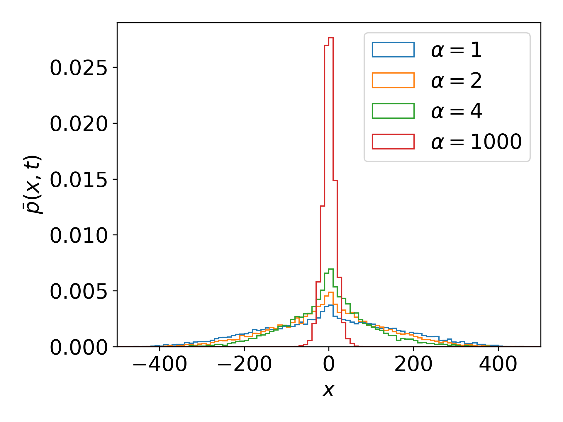
Fig. 1 illustrates the solution (17) obtained by Monte Carlo simulations for the symmetrical case (). One can see the unusually strong dispersion for the subdiffusive master equation, which is a result of the interaction between ensemble self-reinforcement described by and heavy-tailed waiting times with divergent mean described by .
IV.1 Monte Carlo simulations
The simulations for all figures were performed in the following way:
- 1.
Initialize particles at . For each particle, the value of is a random variable drawn from a Beta distribution.
- 2.
Then, for each particle, draw a value for from Mittag-Leffler distributed random numbers. Then where and .
- 3.
Iterate until a required end time .
Mittag-Leffler distributed random numbers were generated using the standard procedure (see (20) in Fulger et al. 2008 or Kozubowski and Rachev 1999).
V Superdiffusion generated by ensemble self-reinforcement
Now, we will show how ballistic superdiffusion can arise due to ensemble self-reinforcement. To do this, we need to find the moments corresponding to the discrete case of (17)
| (22) |
Here, the summation is over all the lattice positions with . Using (10), we can rewrite (22) as
| (23) |
Recognizing that the summation in (23) is simply the mth moment of the discrete random walk, , governed by (8) for any fixed value of , we find
| (24) |
First, we find the conditional moments of the underlying random walk for fixed : and , where is the probability generating function Cox and Miller 1965. Performing this calculation, we obtain
| (25) |
and
| (26) |
The variance is proportional to :
| (27) |
Now, we take the average of (25) and (26) to obtain the variance of the effective random walk. In contrast to (27), the variance involves a term proportional to
| (28) |
where
| (29) |
The difference between (27) and (28) is fundamentally important because the term proportional to generates ballistic superdiffusion
V.1 Symmetric Beta distribution: zero average advection
To avoid the averaged advection caused by an asymmetric Beta distribution, we only consider cases when the Beta distribution is symmetric,
| (30) |
The absence of averaged advection is emphasised in Fig. 1, which shows symmetric distributions for different values of . Figure 1 also shows that in the limit of large , the distribution reverts back to the distribution typical for the subdiffusive regime.
For the symmetric case with , one can obtain
| (31) |
The reason why the variance has a term proportional to can be explained by ensemble self-reinforcement expressed by the transition probabilities in (14), which leads to a greater dispersion of particles over time compared to standard random walks. Note that this result can be obtained by also finding the moments through a recursion relation from the master equation (12) Budini 2016.
One can find the variance for the effective continuous-time random walk
| (32) |
where is defined in (19), and are derived from the fractional Poisson process Laskin 2003 as
| (33) |
and
| (34) |
where
| (35) |
Finally, the variance in continuous time is
| (36) |
The appearance of superdiffusion is demonstrated by numerical simulations in Figs. 2 and 3. Figure 2 demonstrates numerically the relation in (36) and (37) since for values of , shows subdiffusion and for values shows superdiffusion. Moreover for , is exactly diffusive. Note that when , becomes a Poisson process with rate and the variance becomes ballistic:
| (37) |
This result is different from the case when an external force combines with the fractional master equation Metzler et al. 1998; Goychuk et al. 2006 where the first moment is and so the second moment becomes . The superdiffusion caused in this new process is a result of a heterogeneous population of particles and this generates ensemble self-reinforcement demonstrated by (14). A simple random walk with bias and fractional rates would be described by (1) where is a constant. Explicitly, the mean position and variance of this random walk conditional on the transition probability are Shlesinger 1974; Metzler et al. 1998; Goychuk et al. 2006
| (38) |
| (39) |
Clearly, (39) exhibits superdiffusive behavior but the terms proportional to disappear when . The reason for this is that the underlying random walk model, , has variance proportional to , as seen in (27). However, (36) exhibits ballistic superdiffusion when because the effective random walk of the ensemble, , has variance (26) proportional to and .

Furthermore, from this new, heterogeneous population model we are able to achieve a smooth transition in time between subdiffusion and superdiffusion. This is evident by increasing the value of . This is intuitive as the symmetric Beta distribution approaches a delta function centered at as and so we recover the standard fractional master equation and the resulting subdiffusion. However when and , we obtain superdiffusion in the long-time limit. This transition between superdiffusion and subdiffusion is demonstrated using computational simulations in Fig. 3.

VI Discussion
Although there is vast literature on strong memory effects in statistical physics Schütz and Trimper 2004; Kumar et al. 2010; Da Silva et al. 2013; Budini 2016; Baur and Bertoin 2016; Pemantle 1988; Han et al. 2021a; Fedotov et al. 2022, many elephant random walk-like models lack the mechanism of how the strong memory is produced. Given that a heterogeneous population of random walkers emulates strong memory, this opens a new avenue for modelling biological processes that display strong memory properties and yet are heterogeneous ensembles of inanimate objects, like organelles and micromolecules. Might it be that nature has developed a mechanism like ensemble self-reinforcement that we demonstrate in (14) as a proxy for strong memory? Such questions have plagued the field of intracellular transport for decades where brainless membrane-bound vesicles seemingly engage in random walks that appear to have correlations caused by strong memory effects Chen et al. 2015; Fedotov et al. 2018. For example, a high value of might represent a higher affinity to attach to the dynein family of motor proteins and therefore the particle moves very directionally towards the cell nucleus whereas a low value of would be a higher affinity to attach to kinesin which moves towards the cell periphery. A value of would imply that a particle may have equal chance to move in either direction.s The relationship between and speed of a vesicle is . So the bias parameter can be obtained from experiments. Heterogeneity in velocities of intracellular vesicles is well-established Flores-Rodriguez et al. 2011; Fedotov et al. 2018; Han et al. 2020. Ensemble self-reinforcement enables the organization of directional movement as an ensemble effect from heterogeneity. Furthermore, we showed that ensemble self-reinforcement can generate ballistic superdiffusion.
This finding also fits nicely with the emerging theory that, in biological processes, the first arrival times of a signal to a cell (or neuron) influence the subsequent system behavior far more than the average arrival times Schuss et al. 2019. With ensemble self-reinforcement the cell can organize the movement of these particles such that it maintains efficiency of transport and overcomes the trapping that occurs in the crowded cytoplasm. We hypothesise that ensemble self-reinforcement is a way that the cell efficiently transports vesicles in a heavily crowded intracellular environment, which has been shown to be subdiffusive Ba et al. 2018; Fedotov et al. 2021.
VII Summary
In this paper, we formulate a fractional master equation with random transition probabilities across the populations of random walkers. This population heterogeneity generates ensemble average transition probabilities that that increase with the number of steps taken previously, which we call ensemble self-reinforcement. These averaged transition probabilities open a new avenue to model strong memory effects through a heterogeneous ensemble of random walkers. Furthermore, we show analytical solutions for the variance and probability density function of the ensemble averaged, effective random walk.
Through this, we establish the connection between random walks with a heterogeneous ensemble and those with strong memory where the transition probability depends on the entire history of steps. We find the ensemble averaged solution of the fractional master equation through subordination involving the fractional Poisson process counting the number of steps at a given time and the underlying discrete random walk with self-reinforcement. We also find the exact solution for the variance which exhibits superdiffusion even as the fractional exponent tends to 1. This paper demonstrates that heterogeneous populations of anomalous random walks can achieve effective transition probabilities describing strong memory, which we call ensemble self-reinforcement. We find that such heterogeneous populations overcomes heavy-tailed waiting times with divergent mean to exhibit ensemble superdiffusion thus revealing an intrinsic advantage of heterogeneity. Moreover, this provides a new mechanism through which seemingly unintelligent systems can exhibit strong memory.
References
- Bouchaud and Georges (1990) J.-P. Bouchaud and A. Georges, Physics reports 195, 127 (1990).
- Metzler et al. (1999) R. Metzler, E. Barkai, and J. Klafter, Physical review letters 82, 3563 (1999).
- Metzler and Klafter (2004) R. Metzler and J. Klafter, Journal of Physics A: Mathematical and General 37, R161 (2004).
- Scalas (2006) E. Scalas, Physica A: Statistical Mechanics and its Applications 362, 225 (2006).
- Henry et al. (2010) B. I. Henry, T. Langlands, and P. Straka, Physical review letters 105, 170602 (2010).
- Klafter and Sokolov (2011) J. Klafter and I. M. Sokolov, First steps in random walks: from tools to applications (OUP Oxford, 2011).
- Mandelbrot and Van Ness (1968) B. B. Mandelbrot and J. W. Van Ness, SIAM review 10, 422 (1968).
- Kubo (1966) R. Kubo, Reports on progress in physics 29, 255 (1966).
- Zwanzig (1973) R. Zwanzig, Journal of Statistical Physics 9, 215 (1973).
- Goychuk and Hänggi (2007) I. Goychuk and P. Hänggi, Physical Review Letters 99, 200601 (2007).
- Shlesinger et al. (1987) M. F. Shlesinger, B. West, and J. Klafter, Physical Review Letters 58, 1100 (1987).
- Zaburdaev et al. (2015) V. Zaburdaev, S. Denisov, and J. Klafter, Reviews of Modern Physics 87, 483 (2015).
- Livina et al. (2005) V. N. Livina, S. Havlin, and A. Bunde, Physical review letters 95, 208501 (2005).
- Piilo et al. (2008) J. Piilo, S. Maniscalco, K. Härkönen, and K.-A. Suominen, Physical review letters 100, 180402 (2008).
- Wolf et al. (2008) M. M. Wolf, J. Eisert, T. S. Cubitt, and J. I. Cirac, Physical review letters 101, 150402 (2008).
- Luchnikov et al. (2020) I. Luchnikov, S. Vintskevich, D. Grigoriev, and S. Filippov, Physical Review Letters 124, 140502 (2020).
- Bressloff and Newby (2013) P. C. Bressloff and J. M. Newby, Reviews of Modern Physics 85, 135 (2013).
- Chen et al. (2015) K. Chen, B. Wang, and S. Granick, Nature Materials 14, 589 (2015).
- Ba et al. (2018) Q. Ba, G. Raghavan, K. Kiselyov, and G. Yang, Cell reports 23, 3591 (2018).
- Fedotov et al. (2018) S. Fedotov, N. Korabel, T. A. Waigh, D. Han, and V. J. Allan, Physical Review E 98, 042136 (2018).
- Huda et al. (2018) S. Huda, B. Weigelin, K. Wolf, K. V. Tretiakov, K. Polev, G. Wilk, M. Iwasa, F. S. Emami, J. W. Narojczyk, M. Banaszak, et al., Nature communications 9, 1 (2018).
- Schütz and Trimper (2004) G. M. Schütz and S. Trimper, Physical Review E 70, 045101 (2004).
- Kumar et al. (2010) N. Kumar, U. Harbola, and K. Lindenberg, Physical Review E 82, 021101 (2010).
- Da Silva et al. (2013) M. Da Silva, J. C. Cressoni, G. M. Schütz, G. Viswanathan, and S. Trimper, Physical Review E 88, 022115 (2013).
- Budini (2016) A. A. Budini, Physical Review E 94, 052142 (2016).
- Baur and Bertoin (2016) E. Baur and J. Bertoin, Physical review E 94, 052134 (2016).
- Pemantle (1988) R. Pemantle, The Annals of Probability pp. 1229–1241 (1988).
- Tejedor et al. (2012) V. Tejedor, R. Voituriez, and O. Bénichou, Physical review letters 108, 088103 (2012).
- Lanoiselée et al. (2018) Y. Lanoiselée, N. Moutal, and D. S. Grebenkov, Nature communications 9, 1 (2018).
- Meyer and Rieger (2021) H. Meyer and H. Rieger, Physical Review Letters 127, 070601 (2021).
- Han et al. (2021a) D. Han, M. A. da Silva, N. Korabel, and S. Fedotov, Physical Review E 103, 022132 (2021a).
- Fedotov et al. (2022) S. Fedotov, D. Han, A. O. Ivanov, and M. A. da Silva, Physical Review E 105, 014126 (2022).
- Han et al. (2021b) D. Han, D. V. Alexandrov, A. Gavrilova, and S. Fedotov, Fractal and Fractional 5, 221 (2021b).
- Ariel et al. (2015) G. Ariel, A. Rabani, S. Benisty, J. D. Partridge, R. M. Harshey, and A. Be’Er, Nature Communications 6, 1 (2015).
- Han et al. (2020) D. Han, N. Korabel, R. Chen, M. Johnston, A. Gavrilova, V. J. Allan, S. Fedotov, and T. A. Waigh, Elife 9 (2020).
- Altschuler and Wu (2010) S. J. Altschuler and L. F. Wu, Cell 141, 559 (2010).
- Muotri et al. (2005) A. R. Muotri, V. T. Chu, M. C. Marchetto, W. Deng, J. V. Moran, and F. H. Gage, nature 435, 903 (2005).
- Lomvardas et al. (2006) S. Lomvardas, G. Barnea, D. J. Pisapia, M. Mendelsohn, J. Kirkland, and R. Axel, Cell 126, 403 (2006).
- Coufal et al. (2009) N. G. Coufal, J. L. Garcia-Perez, G. E. Peng, G. W. Yeo, Y. Mu, M. T. Lovci, M. Morell, K. S. O’Shea, J. V. Moran, and F. H. Gage, Nature 460, 1127 (2009).
- Zhu et al. (2021) H. Zhu, Q. Li, T. Liao, X. Yin, Q. Chen, Z. Wang, M. Dai, L. Yi, S. Ge, C. Miao, et al., Nature Methods 18, 788 (2021).
- Fedotov et al. (2021) S. Fedotov, D. Han, A. Y. Zubarev, M. Johnston, and V. J. Allan, Philosophical Transactions of the Royal Society A 379, 20200317 (2021).
- Fox et al. (2021) Z. R. Fox, E. Barkai, and D. Krapf, Nature communications 12, 1 (2021).
- Hughes (1995) B. Hughes, Random walks and random environments, volume 1: Random walks clarendon (1995).
- Hughes (1996) B. Hughes, Random walks and random environments, volume 2:random environments (1996).
- Fedotov and Han (2019) S. Fedotov and D. Han, Physical review letters 123, 050602 (2019).
- Flores-Rodriguez et al. (2011) N. Flores-Rodriguez, S. S. Rogers, D. A. Kenwright, T. A. Waigh, P. G. Woodman, and V. J. Allan, PloS one 6, e24479 (2011).
- Wang et al. (2012) B. Wang, J. Kuo, S. C. Bae, and S. Granick, Nature materials 11, 481 (2012).
- Chubynsky and Slater (2014) M. V. Chubynsky and G. W. Slater, Physical review letters 113, 098302 (2014).
- Jain and Sebastian (2016) R. Jain and K. L. Sebastian, The Journal of Physical Chemistry B 120, 9215 (2016).
- Metzler (2020) R. Metzler, The European Physical Journal Special Topics 229, 711 (2020).
- Grebenkov et al. (2021) D. S. Grebenkov, V. Sposini, R. Metzler, G. Oshanin, and F. Seno, New Journal of Physics 23, 023014 (2021).
- Sandev et al. (2022) T. Sandev, V. Domazetoski, L. Kocarev, R. Metzler, and A. Chechkin, Journal of Physics A: Mathematical and Theoretical 55, 074003 (2022).
- Chechkin et al. (2005) A. V. Chechkin, R. Gorenflo, and I. M. Sokolov, Journal of Physics A: Mathematical and General 38, L679 (2005).
- Korabel and Barkai (2010) N. Korabel and E. Barkai, Physical review letters 104, 170603 (2010).
- Berry and Soula (2014) H. Berry and H. A. Soula, Frontiers in physiology 5, 437 (2014).
- Heinsalu et al. (2007) E. Heinsalu, M. Patriarca, I. Goychuk, and P. Hänggi, Physical review letters 99, 120602 (2007).
- Feller (1971) W. Feller, An introduction to probability theory and its applications, vol. 1 (1971).
- Laskin (2003) N. Laskin, Communications in Nonlinear Science and Numerical Simulation 8, 201 (2003).
- Fulger et al. (2008) D. Fulger, E. Scalas, and G. Germano, Physical Review E 77, 021122 (2008).
- Kozubowski and Rachev (1999) T. J. Kozubowski and S. T. Rachev, Journal of Computational Analysis and Applications 1, 177 (1999).
- Cox and Miller (1965) D. R. Cox and H. D. Miller, The theory of stochastic processes (Chapman and Hall, 1965).
- Metzler et al. (1998) R. Metzler, J. Klafter, and I. M. Sokolov, Physical Review E 58, 1621 (1998).
- Goychuk et al. (2006) I. Goychuk, E. Heinsalu, M. Patriarca, G. Schmid, and P. Hänggi, Physical Review E 73, 020101 (2006).
- Shlesinger (1974) M. F. Shlesinger, Journal of Statistical Physics 10, 421 (1974).
- Schuss et al. (2019) Z. Schuss, K. Basnayake, and D. Holcman, Physics of life reviews 28, 52 (2019).