Conformal Freeze-In, Composite Dark Photon, and Asymmetric Reheating

In this section, we describe our UV theory and its RG evolution in a form of cascade confinement. The overall picture is depicted in Figure 1.

In the UV, our theory consists of a sector of CFT (denoted as $\text{CFT}_{1}$) coupled to a sector of elementary (as opposed to composite) particles. The elementary sector includes the inflaton $\Phi$ and a copy of the SM particle contents. The relevant particle contents and their interactions can be summarized by

where

• 1.

  $\mathcal{L}_{\rm ext}$ represents terms for the external “SM” fields, $q=\text{quark},\ell=\text{lepton},A_{\mu}=\{G_{\mu}^{a},W_{\mu}^{i},B_{\mu}\}=\text{gauge fields}$¹¹ 1 Here, we do not include the SM Higgs as we wish to solve the EW hierarchy problem by treating the Higgs as composite. This, however, is not a necessary component of the model.. These are not yet the SM fields. As described below, the SM fields are realized as admixtures of external (elementary) and composite states, i.e. partial compositeness (PC), at energy scale below the confinement scale of $\text{CFT}_{1}$ by diagonalizing the elementary–composite mixing. Such a scheme is commonly used in the so called holographic Composite Higgs Model (CHM). For convenience, we will refer to the combination of external SM fields and the composite states they mix with as the CHM sector.

• 2.

  $\mathcal{L}_{\rm\scriptscriptstyle GW_{1}}=\eta\mathcal{O}_{\rm\scriptscriptstyle GW_{1}}$ describes a scalar deformation responsible for the running of the $\text{CFT}_{1}$ and generation of stable mass gap in the IR. This is the CFT dual of the Goldberger-Wise stabilization mechanism in 5d Goldberger:1999uk and more details can be found in Arkani-Hamed:2000ijo; Rattazzi:2000hs; Agashe:2016rle.

• 3.

  $\mathcal{L}_{\rm\scriptscriptstyle RH}$ describes the interaction between the inflaton $\Phi$ and elementary fields, hence the reheating of the external sector. We emphasize that the inflaton is purely (or mostly) elementary with no (or little) composite mixture and hence it primarily couples only to the external sector.

• 4.

  $\mathcal{L}_{\rm\scriptscriptstyle PC}=y_{q}\bar{q}\mathcal{O}_{q}+y_{\ell}\bar{\ell}\mathcal{O}_{\ell}+gA_{\mu}J_{\mu}+\frac{1}{M_{\rm pl}}h_{\mu\nu}T^{\mu\nu}_{\rm\scriptscriptstyle CFT_{1}}$ represents the linear interactions between the external fields and the CFT operators. When the $\text{CFT}_{1}$ confines in the IR, these will turn into the partial compositeness couplings between elementary fields and their composite partners.

The scalar deformation, $\mathcal{O}_{\rm\scriptscriptstyle GW_{1}}$, triggers RG running of $\text{CFT}_{1}$ and the conformal invariance breaking effect grows in the IR if it is a relevant operator. Eventually, at a scale $\Lambda_{1}$, it becomes an $\mathcal{O}(1)$ violation and leads to a spontaneous breaking of $\text{CFT}_{1}$ measured by the vacuum expectation value (vev) of $\mathcal{O}_{\rm\scriptscriptstyle GW_{1}}$. We assume that $\text{CFT}_{1}$ confines when this occurs. This event generates heavy composite particles which mixes linearly with the external fields. Upon diagonalizing this mass mixing, one gets mass eigenstates including massless states and these are identified as the SM particles. Heavy mass eigenstates correspond to the Kaluza-Klein (KK) excitations in the dual 5d picture.

In addition to the CHM sector described above, we assume that the confinement of $\text{CFT}_{1}$ also gives rise to a sector of composite “preons” which are singlets of the SM gauge group. These preons are similar to the quarks and gluons of QCD, and we assume that their dynamics bring them to an IR fixed point (denoted as $\text{CFT}_{2}$). ²² 2 Strictly speaking, the preon sector needs not be a CFT sector. For our purposes, it suffices that the dynamics of the composite preon sector has a slow RG running and an interacting IR fixed point at a much lower scale (this is our dark CFT). Provided this assumption, all our discussion below will be equally applicable. The dynamics of $\text{CFT}_{1}$ and the phase transition may result in various couplings between the CHM sector and $\text{CFT}_{2}$. We assume that the dominant interaction is given by

where $\rho_{B\mu}$ is the composite $U(1)_{Y}$ vector meson which couples to SM singlet composite fermions (preons) $\psi_{L}$ and $\chi_{R}$ via a dipole interaction. These latter SM singlet composite fermions couple to the $\text{CFT}_{2}$ through the linear mixing couplings. Since $B^{\mu}$ is external to the $\text{CFT}_{1}$, its coupling to the $\text{CFT}_{2}$ (which belongs to the composite sector) has to be through its mixing with composite partner $\rho_{B}^{\mu}$. This mixing is analogous to the $\gamma\text{--}\rho$ mixing realized in QCD and is given by $g/g_{1s}$, where $g$ and $g_{1s}$ are the $U(1)_{Y}$ gauge couping and composite coupling of confined $\text{CFT}_{1}$, respectively. See Agashe:2016rle for more discussion.

Below $\Lambda_{1}$, the above theory will undergo RG flow and the details depend on the scaling dimensions of the fermionic operators of $\text{CFT}_{2}$, $\mathcal{O}_{L,R}$. Denoting the scaling dimensions of these as $d_{L}$ and $d_{R}$ respectively, we first consider $d_{L},d_{R}>5/2$.

In this section, starting from Equation 7, we explain the mass gap generation, IR effective theory below the mass gap $m_{\rm gap}$ and comment on notable features of our model.

We first note that since our model is based on a tensor operator, the RG running of the CFT and dynamical mass scale generation do not go through the mechanisms introduced in Hong:2019nwd; Hong:2022gzo. In particular, the operator mixing effects Hong:2022gzo which makes the COFI-mechanism generic for the case of scalar operator do not occur in our model. Instead, a necessary scalar deformation may arise from the operator product expansion (OPE) $\mathcal{O}_{\mu\nu}\times\mathcal{O}^{\mu\nu}$. We discuss this in detail in Appendix A. Here, we simply assume that such a scalar CFT operator exists and explore its implications on the IR EFT.

If such a deformation is close to being marginal, the theory described by Equation 7 undergoes a slow RG running (walking). At $E\sim m_{\rm gap}$, the conformal invariance is spontaneously broken and a gap scale is generated. By virtue of walking, the separation between $\Lambda_{2}$ and $m_{\text{gap}}$ are generically large.

We make a simplifying assumption that the spontaneous conformal symmetry breaking is a confining phase transition and a spectrum of composite hadrons become the relevant degrees of freedom in the IR. The operator $\mathcal{O}^{\mu\nu}$ is then interpolated by⁶⁶ 6 In principle, the operator can have a non-zero overlap with a composite 2-form field $C_{\mu\nu}$. For our purposes, it suffices to assume that $\mathcal{O}_{\mu\nu}$ has unsuppressed overlap with kinetic term of composite dark photon.

where $\rho_{\mu\nu}$ is the field strength of the composite vector meson $\rho^{\mu}$; the dark photon in our theory⁷⁷ 7 Strictly speaking, the dark photon is a mixture of $A_{D}$ and $\rho$, but it will be mostly comprised of $\rho$. The dependence on $m_{\rm gap}$ is fixed by dimensional analysis and $g_{s}\sim\frac{4\pi}{\sqrt{N}}$ is the coupling constant among the composite states, where $N$ is the number of “color” of the gauge group in the CFT.

The confined phase of the dark CFT may contain a (or a set of) Goldstone boson $\pi$ and they can play the role of dark matter in our theory. Using Equation 10, we obtain the IR effective theory of hadrons from Equation 7

with the kinetic mixing given by

We will now make a few comments on the low energy effective theory. The effective kinetic mixing $\epsilon$ shown in Equation 12 is naturally small. In particular, in addition to the small $\lambda$ (whose natural smallness was explained earlier), it gets further suppressed by the RG running factor $\left(\frac{m_{\rm gap}}{\Lambda}\right)^{d-2}$ (recall $d\geq 2$ by unitarity). This latter factor exhibits the interesting fact that a smaller $m_{\rm gap}$ implies a smaller mixing $\epsilon$. This has a straightforward physics interpretation. We first note that $m_{\rm gap}$ is a consequence of conformal invariance breaking effect, thus the size of $m_{\rm gap}$ is positively correlated with the size of the breaking. In general, a smaller $m_{\rm gap}$ means slower (hence longer) RG running of the CFT sector. On the other hand, the mixing, $\epsilon$, is induced from the coupling between the SM and CFT sectors in the UV theory. The unitarity bound $d\geq 2$ implies that the interaction Equation 7 is an irrelevant operator. This in turn suggests that smaller $m_{\rm gap}$ results in larger suppression of $\epsilon$ from longer RG running.

In addition to the kinetic mixing between the dark photon and hyper-charge gauge boson, we included terms for the dark matter candidate, $\pi^{\pm}$, and their interaction with the dark photon. Here, we assume that dark matter particles are pseudo-Nambu-Goldstone bosons (pNGB) of the spontaneously broken global symmetry of the CFT. Their mass is controlled by the size of the explicit breaking of the global symmetry, which we take to be a free parameter. The ratio $r\equiv m_{\text{DM}}/m_{\rm gap}$ can be smaller than one, which ensures that dark matter can easily be lightest stable particle⁸⁸ 8 From the form of the effective Lagrangian, we’ve implicitly assumed that $\pi$ has a dark charge which ensures stability. If we assumed no such dark charge, then one might expect $\mathcal{O}^{\mu\nu}$ can also interpolate to an operator of the form $\sim\pi\rho^{\mu\nu}$. After kinetic mixing, this will allow the process $\pi\rightarrow\gamma\gamma$. However, the LO decay rate will go as $\epsilon^{4}$; ensuring that its cosmologically long-lived..

Dark matter will couple to the dark photon in the same manner as the pions in low energy QCD interact with the $\rho$-meson. The strength of the coupling is $g_{s}\sim\frac{4\pi}{\sqrt{N}}$. For a reasonable choice of $N$ consistent with large-$N$ treatment, we can take $g_{s}\sim\mathcal{O}(1)$. This coupling induces self-interaction among dark matter states. For $m_{\rm gap}\lesssim\mathcal{O}(100){\rm MeV}$ there are non-trivial constraints on this DM self-interaction, e.g. from observation of the bullet cluster. As we discuss later in subsection 3.4 (also discussed in Hong:2019nwd; Hong:2022gzo), this constraint can be avoided with a proper choice of the ratio $m_{\text{DM}}/m_{\rm gap}<1$. Furthermore, any relevant processes involving the visible sector and the dark matter candidate is independent of $g_{s}$.

Other than the DM particles, the rest of the hadrons in the confined CFT are expected to have mass on the order of $m_{\rm gap}$, which we assume to hold for our model. In particular, the dark photon, as one of the normal composite states, is assumed to have mass $\sim m_{\rm gap}$. We suppress the rest of the hadrons from our effective theory.

The details of the freeze-in production of dark matter in this model depend on the nature of the coupling in Equation 7, especially the scaling dimension $d$ of the operator $\mathcal{O}^{\mu\nu}$. At the same time, it also depend on various scales in the problem, including the temperature in the SM sector $T$, the temperature in the dark sector $T_{\rm ds}$, $m_{\rm gap}$, and the dark matter mass $m_{\rm DM}$.

If the temperature of the SM sector $T$ is larger than $m_{\rm gap}$, then the freeze-in processes produce CFT objects in the final state. We denote this as COFI production. In the other regime, $T<m_{\rm gap}$, the final state consists of the “hadronic” states of the confined CFT and the physics becomes that of standard particle production.

The dark sector is assumed to thermalize with itself.⁹⁹ 9 This condition can easily be satisfied in large-$N$ CFT. Specifically, since we consider non-thermal freeze-in production, our conformal dark sector is a CFT at very low temperature which is strongly interacting. This also allows us to use AdS/CFT duality. When the dark sector is radiation-like, its temperature, $T_{\text{ds}}$, is given by

where $A$ is the analog of $\frac{\pi^{2}}{30}\times{\rm dof}$ appearing in the energy density of a relativistic fluid.

As shown in Hong:2019nwd, IR-dominant COFI production can occur if the sum of the scaling dimensions of the operators appearing in the interaction term Equation 7 is less than or equal to 9/2. In our case, this requires $2<d<5/2$, where the lower limit is the unitarity bound. However, as we will show, this conclusion is based on the assumption that the dark sector is thermalized to a temperature $T_{\text{ds}}>m_{\text{DM}}$ during COFI production. In order to clarify this point, let us first briefly review the COFI production, obtain the bound $d<5/2$, and generalize it to the case $T_{\text{ds}}<m_{\text{DM}}$.

Based on the discussion in subsection 3.1, we are in a position to compute relic abundances of dark matter and study its dependence on various parameters in this model. As is clear from Equation 7, the physics of COFI is controlled mainly by two parameters, $\lambda$ and the scaling dimension $d$ of the CFT operator. These can be traded with $m_{\rm gap}$ and $d$ (see the discussion around Equation 48 and Equation 49). These parameters will be scanned over in our plots. The remaining model parameters: $T_{R}$, $\Lambda$, $r$, and $A$, are fixed for the plots. We are mainly interested in $T_{R}\approx\Lambda\sim\mathcal{O}(\text{TeV})$; with $T_{R}<\Lambda$ to ensure the validity of the theory throughout the entire freeze-in process and asymmetric reheating. The dependence on $A$ is pretty mild. We consider two choices for $r$: $r=0.1$ and $r=0.01$. Finally, depending on scaling dimension $d$, we have two qualitatively different scenarios. We begin with the so called IR-dominant case, with $2<d<2.5$, leaving the UR-dominant production to the next subsection.

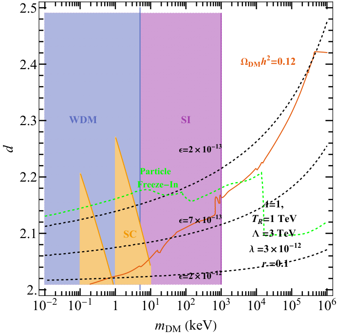
The contours of the observed relic density in the plane of $(m_{\text{DM}},d)$ (with the remaining parameters fixed) is shown in orange-red in Figure 3. For both panels, there is a general tendency for $d$ to increase with $m_{\text{DM}}$. The physics behind this is that as $m_{\text{DM}}$ increases, so does $T_{\rm NR}$ This in turn means that $\rho_{\rm ds}$ starts redshifting as matter at a higher temperature; leading to an effective increase of the final relic density, $\rho_{\rm ds,0}$. This increase must be compensated for by adjusting $d$ so that $\rho_{\rm ds,0}$ matches a constant observed value. A larger $d$ corresponds to a more irrelevant interaction, hence slower heating. Therefore, an increase in $m_{\text{DM}}$ is generically balanced by an increase in $d$, as observed in Figure 3. Following this discussion, one can also determine how the general trend of the contour will behave as we lower our choice $\lambda$ (or equivalently raising $\Lambda$). The scattering process will inject less energy into the dark sector. To compensate, $m_{\text{DM}}$ can be raised so the dark sector can start redshifting as matter earlier or $d$ can be lowered to make the interaction more relevant. As such, the contour will shift towards the bottom right.

Both plots exhibits some sharp change of slope for large $m_{\text{DM}}$. In the case of the left plot, it plateaus; whereas the right plot drops sharply. Both of these correspond to the case with $T_{\text{NR}}=T_{R}$. This can be verified by following the red curve in Figure 4. As discussed in subsubsection 3.1.2, this results in the late time energy density becoming independent of $m_{\text{DM}}$. The discrepancy in the $r=0.01$ plot is due to the fact that $T_{\text{SM}}=m_{\text{gap}}$ and $m_{p}(T_{\text{SM}})=m_{\text{gap}}$ occur at scales close to $T_{R}$. When this happens, the first term in Equation 23 cannot be ignored and the interplay between the two terms determines the overall shape.

A sharp change of slope also occurs for low $m_{\text{DM}}$: at $m_{\text{DM}}\approx 50~\text{keV}$ for the plot and $m_{\text{DM}}\approx 5~\text{keV}$ for the right figure. This is a result of $T_{\text{NR}}$ dropping below the other possible endpoints of production. This can be verified by checking that the intersection of the blue curve with the black curve in Figure 4 does indeed occur at $m_{\text{DM}}\approx 50~\text{keV}$ for $r=0.1$.

There are several localized bumps and dips in Figure 3. They arise from jumps in the number of relativistic degree of freedom, $g_{*}$, and the number of production channel. We explain this focusing on the left panel (with $r=m_{\text{DM}}/m_{\rm gap}=0.1$), but our discussion applies in general.

For example, there are noticeable bumps at $m_{\text{DM}}\approx$ MeV, $d\approx 2.16$. These features are related to $T_{\rm NR}$ crossing some mass threshold: $\Lambda_{\rm QCD}$ followed by $m_{\mu}$ for the subsequent bump. This fact can be checked by finding the intersection of the yellow curve with the purple dashed line in Figure 4.

To understand this better, we note that $T_{\rm NR}$ decreases as we lower $m_{\text{DM}}$. When $T_{\text{NR}}$ happens to cross a threshold, e.g. the electron mass, there are potentially two effects. First, it reduces the number of production channels, effectively decreasing $\rho_{\rm ds,0}$. This must be compensated for by decreasing $d$ which has an effect of increasing the rate of heating, and hence the final energy density. The second effect is the change of $g_{*}$. We incorporated the change of $g_{*}$ numerically by evaluating the energy density exactly outside of any phase transitions, hence the “jump” in $g_{*}$ across each mass threshold (except the QCD phase transition and neutrino decoupling) is rather smoothed out. The (smooth) decrease in $g_{*}$ results in increase in $\rho_{\rm ds,0}$, which then needs to be balanced by increasing $d$. This explains the smooth rising section right after the drop.

During the QCD phase transition, $g_{*}$ drops sharply (increase in $\rho_{\rm ds,0}$) and the up, down, and strange quarks decouple (decreasing the production channels, hence $\rho_{\rm ds,0}$). Numerically, it turns out that the former effect dominates and is compensated by a sharp increase in $d$. Soon after, the muon decouples. This time, the effect of decreasing the number of production channels is larger; requiring a decrease in $d$.

While the qualitative feature described above is solid, the details of the shape appearing in Figure 3 is partly due to the way we implemented $g_{*}$ and changes in the production channel. Furthermore, the impacts of neglecting the derivative of $g_{*}$ in the BE can be large. As such, the shape of the contours in that region should not be taken to be exact.

For comparison, we have also drawn an estimate for the relic density contour for the particle freeze-in scenario based on the results given in Blennow:2013jba in green¹⁶¹⁶ 16 The exclusion contours shown in the figure do not apply to this contour.. To obtain this curve, we assumed that the kinetic mixing parameter is given by Equation 12 and the dark photon mass obeys $rm_{A^{\prime}}=m_{\text{DM}}$. Using the right plot as an example, for low dark matter masses, we see that the contour exactly follows the contour of constant kinetic mixing parameter. As $m_{\text{DM}}$ increases, the contour is interpolated to another contour of constant kinetic mixing parameter. This is due to the increase in $g_{*}(m_{A^{\prime}})$ which needs to be compensated for by increasing the kinetic mixing. This illustrates that the predictions for COFI is very different from that of the particle dark photon scenario.

The contours of the observed relic density in the plane of $(m_{\text{DM}},\lambda)$ (with the remaining parameters fixed¹⁷¹⁷ 17 For a fixed $d$, changes to $T_{R}$ and $\Lambda$ consistent with $T_{R}<\Lambda$ is equivalent to redefining $\lambda$.) is shown in Figure 5. In both plots, we see the same behavior: two straight lines with constant, negative slope.

The physics of this scenario is simpler to describe compared to the IR-dominant freeze-in scenario. When $d>5/2$, the $T_{R}$-dependent terms become the dominant contribution to the relic density at low temperatures. If the dark sector temperature increases rapidly beyond $m_{\text{DM}}$ by the initial energy transfer, we can safely drop the $T^{2d-5}$ term in Equation 21 and the energy density is of the form constant$\times T^{4}$. This tells us that the energy transfer from the SM sector has concluded and the dark sector energy density simply redshifts as radiation. This continues until the dark matter becomes non-relativistic, which occurs at

The energy density then continues to redshift as matter until today. This gives

Factoring out the $m_{\text{DM}}$ and $\lambda$ dependence, we see

So a log-log contour plot of constant $\rho$ will look like a straight line.

In the case where the dark sector was never relativistic, the energy density today is simply

Here, we see that the relic density is independent of the dark matter mass¹⁸¹⁸ 18 Just like in the case of the IR-dominant production, there are higher order corrections which do depend on the dark matter mass.. Thus, a contour plot of fixed $\rho$ is simply a flat line in $\lambda$

In this section, we discuss experimental as well as theoretical constraints on our model. Ones with non-trivial restrictions on the allowed parameter space are included in the plots of our main results Figure 3 and Figure 5.

References

- (1) M. Battaglieri et al., US Cosmic Visions: New Ideas in Dark Matter 2017: Community Report, in U.S. Cosmic Visions: New Ideas in Dark Matter, 7, 2017 [1707.04591].
- (2) J. Alexander et al., Dark Sectors 2016 Workshop: Community Report, 8, 2016 [1608.08632].
- (3) J. McDonald, Thermally generated gauge singlet scalars as selfinteracting dark matter, Phys. Rev. Lett. 88 (2002) 091304 [hep-ph/0106249].
- (4) L.J. Hall, K. Jedamzik, J. March-Russell and S.M. West, Freeze-In Production of FIMP Dark Matter, JHEP 03 (2010) 080 [0911.1120].
- (5) S. Hong, G. Kurup and M. Perelstein, Conformal Freeze-In of Dark Matter, Phys. Rev. D 101 (2020) 095037 [1910.10160].
- (6) S. Hong, G. Kurup and M. Perelstein, Dark Matter from a Conformal Dark Sector, 2207.10093.
- (7) W.D. Goldberger and M.B. Wise, Modulus stabilization with bulk fields, Phys. Rev. Lett. 83 (1999) 4922 [hep-ph/9907447].
- (8) N. Arkani-Hamed, M. Porrati and L. Randall, Holography and phenomenology, JHEP 08 (2001) 017 [hep-th/0012148].
- (9) R. Rattazzi and A. Zaffaroni, Comments on the holographic picture of the Randall-Sundrum model, JHEP 04 (2001) 021 [hep-th/0012248].
- (10) K. Agashe, P. Du, S. Hong and R. Sundrum, Flavor Universal Resonances and Warped Gravity, JHEP 01 (2017) 016 [1608.00526].
- (11) R. Contino, The Higgs as a Composite Nambu-Goldstone Boson, in Theoretical Advanced Study Institute in Elementary Particle Physics: Physics of the Large and the Small, pp. 235–306, 2011, DOI [1005.4269].
- (12) K. Agashe, S. Hong and L. Vecchi, Warped seesaw mechanism is physically inverted, Phys. Rev. D 94 (2016) 013001 [1512.06742].
- (13) C. Dvorkin, T. Lin and K. Schutz, Making dark matter out of light: freeze-in from plasma effects, Phys. Rev. D 99 (2019) 115009 [1902.08623].
- (14) M. Blennow, E. Fernandez-Martinez and B. Zaldivar, Freeze-in through portals, JCAP 01 (2014) 003 [1309.7348].
- (15) V. Iršič et al., New Constraints on the free-streaming of warm dark matter from intermediate and small scale Lyman- forest data, Phys. Rev. D 96 (2017) 023522 [1702.01764].
- (16) A. Berlin, N. Blinov, G. Krnjaic, P. Schuster and N. Toro, Dark Matter, Millicharges, Axion and Scalar Particles, Gauge Bosons, and Other New Physics with LDMX, Phys. Rev. D 99 (2019) 075001 [1807.01730].
- (17) J. Kaplan, Lectures on AdS/CFT from the Bottom Up, 2207.10093.
- (18) L. Randall and R. Sundrum, A Large mass hierarchy from a small extra dimension, Phys. Rev. Lett. 83 (1999) 3370 [hep-ph/9905221].
- (19) L. Randall and R. Sundrum, An Alternative to compactification, Phys. Rev. Lett. 83 (1999) 4690 [hep-th/9906064].
- (20) K.S. Agashe, J. Collins, P. Du, S. Hong, D. Kim and R.K. Mishra, LHC Signals from Cascade Decays of Warped Vector Resonances, JHEP 05 (2017) 078 [1612.00047].
- (21) K. Agashe, J.H. Collins, P. Du, S. Hong, D. Kim and R.K. Mishra, Dedicated Strategies for Triboson Signals from Cascade Decays of Vector Resonances, Phys. Rev. D 99 (2019) 075016 [1711.09920].
- (22) K. Agashe, J.H. Collins, P. Du, S. Hong, D. Kim and R.K. Mishra, Detecting a Boosted Diboson Resonance, JHEP 11 (2018) 027 [1809.07334].
- (23) K. Agashe, M. Ekhterachian, D. Kim and D. Sathyan, LHC Signals for KK Graviton from an Extended Warped Extra Dimension, JHEP 11 (2020) 109 [2008.06480].
- (24) R. Contino, T. Kramer, M. Son and R. Sundrum, Warped/composite phenomenology simplified, JHEP 05 (2007) 074 [hep-ph/0612180].
- (25) B. Grinstein, K.A. Intriligator and I.Z. Rothstein, Comments on Unparticles, Phys. Lett. B 662 (2008) 367 [0801.1140].
- (26) G.G. Raffelt, Stars as laboratories for fundamental physics: The astrophysics of neutrinos, axions, and other weakly interacting particles, University of Chicago Press (5, 1996).
- (27) J.H. Chang, R. Essig and S.D. McDermott, Supernova 1987A Constraints on Sub-GeV Dark Sectors, Millicharged Particles, the QCD Axion, and an Axion-like Particle, JHEP 09 (2018) 051 [1803.00993].