Measurement of Hadron Production
in Interactions at 158 and 350
with \NASixtyOneat the CERN SPS
\PreprintIdNumberCERN-EP-2022-194
\ShineJournalPhys. Rev. C
\ShineAbstract
We present a measurement of the momentum spectra
of , K±, p±, , and K produced in
interactions of negatively charged pions with carbon nuclei at beam
momenta of 158 and 350 . The total production cross sections are
measured as well. The data were collected with the large-acceptance
spectrometer of the fixed target experiment \NASixtyOneat the CERN
SPS. The obtained double-differential - spectra provide a unique
reference data set with unprecedented precision and large phase-space
coverage to tune models used for the simulation of particle production
in extensive air showers in which pions are the most numerous
projectiles.
1 Introduction
When cosmic rays collide with the nuclei of the atmosphere, they initiate a cascade of secondary particles called air shower. The interpretation of cosmic-ray data from air-shower arrays such as KASCADE-Grande [1], IceTop [2], Telescope Array [3] or the Pierre Auger Observatory [4] relies to a large extent on the understanding of these particle cascades in the atmosphere, specifically on the correct modeling of hadron-air interactions that occur during shower development. However, it is a well-established fact that air shower simulations using current state-of-the-art models of high-energy hadronic interactions produce significantly less muons than observed in data [5, 6, 7, 8, 9, 10, 11, 12, 13, 14, 15, 16, 17].
The majority of muons in air showers are created in decays of charged pions when the energy of the pion is low enough such that its decay length is smaller than its interaction length in air. The projectiles creating these pions are typically produced at equivalent beam energies below a TeV [18, 19, 20] which is well within the reach of current accelerators. However, only a very limited amount of data exists on the interactions of the most numerous projectile in air showers, the -meson [21].
In this paper, we present new data from the \NASixtyOneexperiment at the CERN SPS on the particle production in interactions of pion beams at 158 and 350 with a thin carbon target (used as a proxy for nitrogen, the most abundant nucleus in air). After a brief introduction to the experiment in Section 2, we will describe the various data analysis steps that lead to the results presented in this paper. These steps are sketched in Fig. 1 for a better orientation of the flow of the analysis and the corresponding sections in which they are described in this article. The processing and selection of data and simulations are introduced in Section 3. The three main analyses of the cross section, decays, and identified charged particles are explained in Sections 4, 5, and 6, respectively. The calculation of the particle spectra and the estimation of their uncertainties is outlined in Section 7, where the measured production spectra of , K±, p±, , and K are presented. In Section 8 we conclude by comparing our measurements to the predictions of hadronic interaction models used for the modeling of air showers.
2 Experimental Setup and Data Taking
The data reported in this paper were taken in 2009 with the \NASixtyOneinstrument, a wide-acceptance hadron spectrometer at the CERN SPS on the H2 beam line of the CERN North Area [22]. The experimental setup used to record interactions is shown in Fig. 2.
The main part of the detector consists of five Time Projection Chambers (TPCs) which were inherited from NA61’s predecessor, the NA49 experiment [23]. Two Vertex TPCs (VTPC-1 and VTPC-2) are located inside the magnetic field produced by two superconducting dipole magnets. For the measurements presented in this paper the two magnets were operated at full electric current providing a field of 1.5 and 1.1 T, respectively. Two Main-TPCs are located downstream of the VTPCs to measure particles bent in the left and right hemispheres (MTPC-L and MTPC-R). An additional small TPC is placed between VTPC-1 and VTPC-2, covering the very-forward region, and is referred to as the gap-TPC (GTPC). The combined bending power of the magnets is 9 T m and the coordinates on a track are measured with a precision of a few 100 m. The resolution of the measurement of particle momenta in the TPCs depends on the track topology, i.e. on the overall track length and the number of position measurements [24]. Typical values for the momentum resolution are for low-momentum tracks measured only in the VTPC-1 ( ) and for tracks traversing the full detector up to the MTPCs ( ).
For the study reported in this paper, the SPS delivered a secondary hadron beam originating from interactions of 400 primary protons impinging on a 10-cm-long beryllium target. The negatively charged hadrons () produced in these interactions were transported through the H2 beam line to the \NASixtyOneexperiment. A beam momentum of 158 was requested for the first part of data taking and 350 for the second part. At these momenta the negatively charged beam particles are mostly mesons. They are identified by a differential ring-imaging Cherenkov detector (CEDAR) [25] and the fraction of pions was measured to be for 158 and for 350 (see Fig. 2 in [26]). The CEDAR signal is recorded during data taking and then used as an offline selection cut.
Downstream of the CEDAR three proportional chambers are used as Beam Position Detectors (BPDs) to measure the trajectories of the incoming particles. Two scintillation counters (S1 and S2) and three veto counters (V0, V1 and V1′) define the beam trigger with the coincidence
| (1) |
see inset in Fig. 2. The beam trigger is a zero bias trigger. Furthermore, an interaction trigger,
| (2) |
is defined as the anti-coincidence of the incoming beam particle and S4, a scintillation counter with a diameter of 2 cm placed between the VTPC-1 and VTPC-2 along the beam trajectory at about 3.7 m from the target. If an inelastic interaction occurs then the produced particles typically have momenta considerably lower than the beam momentum and are thus bent away from the beam trajectory such that no particle reaches S4. The anti-coincidence with S4, therefore, serves as a minimum-bias interaction trigger.
During data taking a prescaled fraction of the and signals can trigger the data acquisition system to read out the TPCs and write a raw event to disk. For most of the data taking period, the pre-scaling was 0.4% for the zero-bias beam trigger and 100% for the minimum-bias interaction trigger.
The target used for this study was an isotropic graphite plate with a thickness along the beam axis of 2 cm and a density of g/cm3, equivalent to about 4% of a nuclear interaction length. 90% of data was recorded with the target inserted and 10% with the target removed. The latter data was used to subtract interactions that took place in the material upstream and downstream of the target. In total, 5.5 million events were recorded with the target inserted at a beam momentum of 158 and 4.5 million events at 350 .
3 Data Processing and Selection
3.1 Reconstruction
The raw data recorded during data taking are processed with the standard \NASixtyOnereconstruction chain (based on tried-and-tested algorithms developed by the NA49 collaboration) to obtain high-level physics information such as the charge and momentum of the produced particles. Firstly, charge clusters are identified in the raw data of the TPCs and their three-dimensional positions are reconstructed from the centroids in drift time and in position on the TPC readout pads. A pattern recognition combines these clusters to form local track segments in each TPC separately. The local track segments are matched to global tracks for which the track parameters (track position at reference plane, charge and three-momentum) are fitted.
The beam trajectory before the target is determined using the position measurements from the BPDs. The position of the nominal main interaction vertex is estimated as the intersection of the reconstructed beam trajectory with a plane located at the center -position of the 2 cm-carbon target. Global tracks compatible with this position are then re-fitted with this vertex hypothesis leading to main-vertex track candidates with track parameters at the nominal interaction vertex. Furthermore, the -position of the main interaction vertex is reconstructed by fitting a common origin of these global tracks along the beam trajectory. Depending on the track multiplicity, the resolution along the -axis for the vertex position obtained in this way exceeds the target thickness, therefore better main-vertex-constrained track-momenta can be obtained by using the nominal interaction vertex in the middle of the target instead. Yet, the reconstructed vertex position is useful for the rejection of obvious out-of-target interactions during the event selection (see below).
In addition to the main-vertex hypothesis, each combination of positively and negatively charged global tracks within one event is investigated for a common origin downstream of the target from the decay of a long-lived neutral particle (so-called events). All pairs with a distance of closest approach cm anywhere along their trajectory downstream of the target are re-fitted with the constraint to originate from a common vertex resulting in candidates that will be analyzed in Section 5.
3.2 Simulation
Through this analysis, we will use simulations of the measurement to correct the raw-data spectra for various distortions originating from the detector acceptance, re-interactions with the detector material and within the target, feed-down from weak decays etc. For this purpose we simulated interactions at both beam momenta with the hadronic event generators Epos 1.99 [29] and QGSJet II-04 [30] with the crmc program [31]. The 1.99 version of the Epos model was used rather than its newer “LHC” variant as the former is better tuned to interactions at SPS energies [32]. The particles produced by these generators are then passed to a simulation of the passage of particles through the material and magnetic field of the \NASixtyOnesetup using the Geant 3.21 package [33]. The hits generated in the active detector volumes are digitized to produce the same raw information as for real data and an interaction trigger is simulated by checking whether any of the charged particles hit the S4 counter. The simulated information is then processed with the same reconstruction algorithms discussed in the previous section and the results are stored in the same output format as the reconstructed data.
3.3 Event Selection
We apply the following event-selection criteria11 1 The event selection criteria used here are identical to the ones described in Ref. [26] for the same data set discussed in this paper. We therefore refer to Sections 2 and 3 of that paper for a detailed description of the event selection. to obtain a set of high-quality interaction triggers.
Pion projectiles are selected with the CEDAR (see previous section) and a pile-up of interactions is avoided by rejecting events in which the S1 scintillator detected another beam particle within s of the time of the interaction trigger. Furthermore, it is required that the direction of the beam was well measured with the three beam position detectors. These three cuts select high-quality projectiles based on measurements from the beam detectors upstream of the target.
Further event selection criteria define the subset of -projectiles with an interaction in the target. Here we analyze the particles produced in events recorded with the minimum-bias trigger. Furthermore, we reject events with an interaction vertex reconstructed far from the center of the target ( cm), since such events mostly originate from interactions outside of the target.
With these criteria we select and minimum-bias triggers recorded with an inserted C-target at 158 and 350 , respectively. By construction, due to the restriction to events with a reconstructed vertex close to the target position, only very few events recorded with a removed target survive the selection ( events in each data set). The sum of simulated events with an inserted target is and for beam momenta of 158 and 350 respectively.
3.4 Track Selection
The set of selection criteria given below is applied to the tracks measured in the TPCs. They are constructed to assure good quality of the momentum measurements and to select regions of the detector with a solid understanding of the detection efficiency.
Track Quality
The total number of clusters on the track must be and the sum of clusters in both VTPCs must be , or the number of clusters in the GTPC must be . These cuts assure a good momentum determination in either the VTPCs within the magnetic field, or a large lever arm for forward tracks measured with a combination of GTPC and MTPC [34].
Fiducial Acceptance
For each particle charge, we restrict the analysis to bins in azimuthal angle, total momentum and transverse momentum, (, , ), in which the track selection efficiency is larger than 90% for simulated tracks.22 2 Since the acceptance is only a property of the track momentum and direction (not of the beam momentum or track multiplicity), it can be determined with high statistical accuracy averaging all available simulation sets. A total of simulated events were used to construct the acceptance map. This number is higher than the sum of simulated events mentioned in Section 3.3, since for the acceptance study we also included events generated with the DPMJet 3.06 model, which were not used otherwise for this study. This cut mainly removes tracks at the edges of the detector for which the efficiency drops rapidly, as illustrated in the example shown in the top-left panel of Fig. 3. Since the TPCs have a larger width than height (cf. lower left panel in Fig. 3), the acceptance is not uniform in and especially poor along . But since neither the beam nor the target are polarized, the particle yields are independent of and we can thus restrict the analysis to regions where the detection efficiency is near 100%. The fiducial volume selected by the acceptance cut therefore leads to a near-geometric acceptance that is given by the number of accepted -bins [34]. The acceptance for positively charged tracks is visualized in Fig. 3.
Origin at Primary Vertex
Furthermore, we require that the distance between the position of the intercept of the extrapolation of the track (reconstructed without vertex-constraint) to the interaction plane and the position of the main interaction vertex must be smaller than 4 cm in both horizontal and vertical direction. This cut removes out-of-target interactions and tracks from particle decays (“feed-down”).
Furthermore, we require that the distance between the extrapolation of the track (reconstructed without vertex-constraint) to the interaction plane and the interaction point must be smaller than 4 cm in both horizontal and vertical direction. This cut removes out-of-target interactions and tracks from particle decays (“feed-down”).
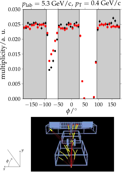

After the track selection, the measured tracks are split into two subsets called right-side tracks (RSTs) and wrong-side tracks (WSTs). The former group is defined as the tracks that bend away from the beam axis, while the latter as the tracks that bend towards the beam axis33 3 The terminology of wrong- and right-side tracks dates back to NA49 and reflects the fact that the tilt angle of the pads in the VTPCs were optimized to measure the right-side topologies., i.e. (RST) and (WST), where and and are the momentum and charge of the track. These conditions simplify to for RSTs and for WSTs for the usual case of forward production in the laboratory frame, . The distinction between the two track topologies is motivated by the fact that a right- and a wrong-side track with the same and , cross different regions of the detector, which has important implications for the particle reconstruction and identification step based on the measurements (see Section 6). Furthermore, this subdivision defines two independent data sets that can be compared to estimate the systematic uncertainties of the measured particle multiplicities, see Section 7.4.2.
4 Cross Section Analysis
The measurement of the production cross section44 4 The production cross section is defined by , where denotes the total cross section, the coherent elastic cross section and the quasi-elastic cross section. Quasi-elastic interactions are processes in which no new particles are produced, but the target nucleus is fragmented. in interactions closely follows the analysis procedure detailed in Ref. [35]. The experimental interaction cross section is measured by counting the number of interaction triggers, , within the recorded zero-bias beam triggers, , to obtain the interaction trigger probability
| (3) |
The interaction probability in the carbon target is then obtained by correcting for out-of-target interactions via
| (4) |
where the trigger probabilities measured with the target removed are denoted by a superscript R and the ones with the target inserted with a superscript I.
The interaction trigger cross section is given by
| (5) |
where is Avogadro’s number and , and are the density, molar mass and length of the target, respectively. The logarithmic term, , accounts for the exponential attenuation of the beam inside the target.
The experimentally accessible interaction trigger cross section can be related to the production cross section by correcting for the residual contributions to originating from elastic and quasi-elastic scattering ( and ). Furthermore, a correction for inelastic interactions, to which the interaction trigger is not sensitive to, is needed
| (6) |
where , , and are the fractions of elastic, quasi-elastic, and production events that lead to an trigger. and thus give the fraction of false-positive interaction triggers from (quasi-)elastic interactions and is the fraction of false-negative production interactions.
| beam momentum | 158 | 350 |
|---|---|---|
| /mb | 0.8 | 0.9 |
| /mb | 0.3 | 0.3 |
| 0.0012 | 0.00 | |
| 0.03 | 0.02 | |
| 0.02 | 0.02 |
We derived model predictions for and by performing a Glauber calculation [36] of interactions using a fit to previously measured cross sections of [37] as an input. The resulting cross sections are listed in Table 1 where the quoted systematic uncertainty originates from different assumption on the inelastic screening in interactions [38].
The fractions depend on the chosen interaction trigger condition. We use the FTFP_BERT physics list of Geant 4.9.4.p01 [39] to estimate and . For systematic checks, we assumed that the angular distribution of quasi-elastic scattering in is very similar to free pion-nucleon scattering and can thus be modeled using the elastic slope in scattering. was estimated by generating interactions with the hadronic models Fluka 2011.2.9 [40], Epos 1.99 [29], QGSJet01 [41], QGSJet II-03 [30], Venus 4.12 [42], Sibyll 2.1 [43] Urqmd 1.3.1 [44, 45] using the INTTEST mode of Corsika [46]. The arithmetic mean of the different predictions of is used to correct the data, and the maximum and minimum values as an estimate of the systematic uncertainty.
In previous cross-section analyses within \NASixtyOnewe used the absence of a signal in the S4 counter to define an interaction. But, as can be seen in Fig. 20 in the appendix, especially for the 350 data studied in this paper, the radius of 1 cm of the S4 would lead to a large model-dependent correction for with Eq. 6. Therefore, we instead use the GTPC to define an offline interaction trigger by requiring the absence of a track within a radius from the beam extrapolation at 3.7 m downstream of the target (i.e. at the -position of the S4 plane, located before the GTPC). We choose the trigger radius which minimizes the quadratic sum of statistical and systematic uncertainty of the measured cross section leading to an of 0.9 and 0.6 cm for beam energies of 158 and 350 respectively, see Ref. [47]. The analysis is performed on the zero-bias beam trigger data with and events at 158 and 350 , respectively, where the number in brackets refers to the data taken with a removed target.
With the above definition of the offline interaction trigger, we find an interaction probability of
| (7) |
and
| (8) |
and the cross section fractions as listed in Table 1.
Evaluating Eq. 6 with the trigger cross section derived via Eq. 5 from these measurements as well as with the correction factors listed in Table 1, leads to our estimates of the production cross section in interactions of
| (9) |
and
| (10) |
The systematic uncertainty includes contributions from the inefficiency of the GTPC, uncertainties of the detector simulation, and the uncertainties of the correction factors quoted in Table 1. The largest contribution of about 3.5 mb originates from the model uncertainty of . In Appendix A we provide the efficiency map corresponding to the two beam energies such that in the future it will be possible to recalculate with a different set of models, and possibly smaller systematic uncertainty.
The obtained cross sections are presented in Fig. 4 along with the theoretical prediction using the Glauber theory [36] for several assumptions on the inelastic screening parameter [38] (from top to bottom , 0.3, 0.5, 0.7 and 0.9) and previous measurements [48, 49, 50, 51, 52].55 5 Here we use Glauber predictions of , and to scale all measurements to . The measurements of from Refs. [50] and [51] are multiplied by and the measurement of from Ref. [49] is multiplied by . As can be seen, the only previous data set on the production cross section in interactions from Ref. [48] agrees well with our measurement and the total uncertainty of the cross sections presented here matches the statistical precision of this old measurement (no systematic error was quoted in this reference). Furthermore, our measurement agrees well with the Glauber predictions for a broad range of inelastic screening assumptions, but small values are disfavored and the preferred range is within .
5 analysis
As a first step of the analysis of particle spectra, we investigate the production of the neutral weakly-decaying particles , and K. The production spectra of these strange particles provide important constraints for the tuning of hadronic interaction models, see e.g. Ref. [53]. Moreover, a good knowledge of these spectra is also important to distinguish particles created directly in interactions from particles originating from weak decays, see Section 7.2.
Neutral weakly decaying particles with an average decay length () of the order of a few to tens of centimeters can be detected by \NASixtyOneexperiment through their charged decay products. This type of particle is traditionally called , because of its neutral charge and the V-shaped decay topology. Although the itself does not create a track in the TPCs, the products of its decay may do, allowing us to reconstruct the position of the decay vertex and, by using the momenta of the daughter tracks, reconstruct the properties of the parent particle.
In Table 2 we list the three particles studied in this work together with the branching ratio of the decay channels investigated here.
| mass [GeV/] | [cm] | decay | branching ratio | ||
|---|---|---|---|---|---|
| 1.1157 | 7.89 | p+ | 63.9 | ||
| 1.1157 | 7.89 | + | 63.9 | ||
| K | 0.4976 | 2.68 | + | 69.2 | |
candidates are selected by calculating the distance of closest approach (dca) for each combination of one positively and one negatively charged track. To assure a good momentum resolution, both tracks should in total have more than 30 clusters each and more than 15 clusters in the VTPCs. Each combination with a cm downstream of the main vertex is re-fitted under a common vertex hypothesis. To increase the signal-to-background ratio, the reconstructed momentum is then extrapolated to the vertex plane and the radial impact parameter, , is required to be cm. Here and denote the coordinates of the impact point in the target plane with respect to the main vertex and the factor accounts for the fact that the resolution in the bending plane is approximately twice as large as in the -plane. The efficiency of this cut is in all of the phase space bins studied here.
A further reduction of the background is possible by selecting events with a reconstructed decay vertex far from the target, as the background arises mostly from combinations involving non- tracks from the main vertex. A large distance cut, , improves the purity of the sample, but also diminishes the selection efficiency, for an ideal detector. Therefore an optimal selection distance that minimizes the uncertainty of the extracted signal is chosen, depending on the particle type and momentum as described in Ref. [54].
For the measurement of the multiplicity of particles, we study the distribution of the invariant mass of combinations of candidate tracks,
| (11) |
in bins of and (cf. Appendix B). Here the subscripts and refer to the positively and negatively charged daughter particles, denote their four-momenta and the reconstructed three-momenta of candidate tracks. Eq. 11 is evaluated for three mass combinations corresponding to the main , and K decays listed in Table 2 and the energies are calculated accordingly via . Examples of invariant mass distributions are shown in Fig. 5. As can be seen, the “real” combinations peak around the mass of the whereas the background of unrelated track combinations exhibits a broad and nearly flat distribution.
The number of s is extracted in a Poissonian likelihood fit [55] describing the invariant mass distribution as the sum of the signal template and the background function. For this purpose, the signal distribution is modeled using the shape of the reconstructed as predicted by the detector simulation and for the background distribution a polynomial function is used. We found that a second-degree polynomial provides a satisfactory description of the data in the chosen interval. A third-degree polynomial was used to estimate the systematic uncertainties of the background shape description (see Section 7.4.2). These signal and background templates are illustrated as blue and red histograms in Fig. 5. The number of s produced in the fitted - bin is then inferred from the normalization of the fitted distributions.
6 analysis
The spectra of identified particles produced at the main vertex are obtained by extracting the average particle yields in each kinematic bin from the measured distributions of the energy loss of tracks in the TPCs. For this purpose, we calculate the truncated mean [56], , of the charges of the 50% of clusters with the lowest charge among the clusters detected along each particle track . As in the Bethe formula [57], depends on and can thus be used to identify particles of different masses at a particular momentum . The two-dimensional distribution of energy deposit and momenta of selected main-vertex tracks at a beam momentum of 158 are displayed in Fig. 6 along with a Bethe-inspired parametrization of the mean energy deposit for the particles considered here, i.e. electrons, pions, kaons, protons, and deuterons and their anti-particles.

An example of the distribution of the of tracks in a particular and bin is shown in Fig. 7 for negatively and positively charged particles. The production yields of different particle types are determined by fitting the distribution with the sum of -templates for electrons, pions, kaons, protons, and deuterons. The shapes of these templates are based on previous studies from \NAFortyNineand \NASixtyOne [58, 59, 60] which describe the distribution of energy deposit of each particle type by the sum of asymmetric Gaussians taking into account the distribution of (number of clusters per track) and the distribution of momenta within the bin.
The fitting is performed using a binned maximum-likelihood method. In the general case, 10 particle fractions (5 particle types and 2 charges) and 10 model parameters are taken as free parameters of the fit. Most of these model parameters are nuisance parameters that allow the mean and width of the distributions to stray away from the global parametrization. In that way, residual systematic offsets of the calibration of cluster charges in different parts of the detector can be corrected.
As illustrated in Fig. 7, in general the -fits lead to a very satisfactory description of the data. The example shown here is close to a momentum where the mean values of protons and kaons as well as the one of electrons and deuterons overlap (cf. Fig. 6). In case of a near-complete degeneracy between the fitting templates of different masses in certain momentum bins (“Bethe crossings”), the fitted yields of these ambiguous particles are excluded from the final results.
7 Derivation of the Particle Spectra
The and analyses described in the previous two sections result in the number of identified tracks (, K±, p, , , , and K) in bins of and for each of the two data taking modes, i.e. with the target inserted and removed. For the choice of binning, see Appendix B.
Given these measurements, the double-differential particle production spectra can be computed for each particle as
| (12) |
This quantity is the track multiplicity per production event in a certain - bin, sometimes also referred to as average multiplicity. Here and denote the widths of the phase-space bin and the transverse component of the momentum vector is defined with respect to the beam direction , . is a correction factor derived from simulations that will be discussed in the next section. The indexes I and R refer to target inserted and removed, respectively, and is the number of selected minimum-bias interaction-trigger events. The factor is the so-called target-removed factor and it normalizes both target inserted and removed data set to the same number of beam particles. Given the number of events, , and the probability of a beam particle to produce an interaction trigger, , the number of beam particles for a given data set can be estimated as . is measured from zero-bias beam triggers, see Eq. 3. The target-removed factor is given by and its value is about five, corresponding to the time spent in target-removed configuration during data taking.
7.1 Correction Factors
The selected number of events and the estimated number of particles in a given phase space bin are biased estimators of the true number of production events and the true number of produced particles . These biases are corrected for with the help of simulations for which it is easy to determine the ratio of generated and measured spectra,
| (13) |
where and are the values from the event generator, and are obtained after the detector simulation, event reconstruction, and event and track selection. Two simulated data sets generated with different hadronic interaction models (see Section 3) are used for systematic studies.
To gain further insights into the different contributions to the correction factor it is useful to split into event- and particle-contribution factors, referred to as and in the following,
| (14) |
The factor is a property of the data set as a whole and thus depends only on the beam energy, whereas the factor depends on the phase space bin and on the particle type. We get and for beam momenta of 158 and 350 , respectively. These values were determined from the arithmetic average of the two simulated data sets, with the upper uncertainty range corresponding to the result predicted by Epos 1.99 and the lower range to the one from QGSJet II-04. These values give the product of the efficiency of the vertex- cut (cf. Section 3.3) and the efficiency of the minimum-bias interaction trigger (cf. Section 2). The former amounts to approximately 0.975 with a good agreement between real and simulated data. Therefore, is dominated by the trigger efficiency and is thus mainly a model-dependent correction, since the efficiency depends on the fraction of events with a high-momentum charged particle triggering the S4 scintillator. Overall, the two hadronic generators used here show a good overall agreement in their predictions of . In the following, we will use the average value for the correction and the difference for systematic uncertainty. A slightly larger uncertainty would result if the standard deviation of efficiencies of all the models shown in Fig. 20 of the appendix would be used as an estimate of the systematic uncertainty. Note that for the majority of phase-space bins, the total correction for the trigger efficiency is small, as it affects both and . The correction is mostly relevant at high momenta when the trigger efficiency affects but not since the conservation of the beam momentum does not allow for the simultaneous presence of a high-momentum particle in the TPCs and another high-momentum particle hitting the S4 scintillator.
The correction factors as a function of and are given by the ratio of the generated and measured number of tracks. They are shown in Fig. 8 for , K±, p±, , , and K. Note that the factors for the s also include the effect of the cuts, presented in Section 5.
The geometrical acceptance of the detector is the dominant contribution to the factor at large . Most of the overall structure visible in the plots is due to the acceptance and reflects the aspect ratio of the TPCs (rectangular in the plane) and the bending of particles in the magnetic field. At particle momenta of , the TPCs provide full coverage for increasing up to at 30 . Due to the requirement on the number of clusters in the different TPCs (cf. Section 3.4), the coverage decreases at higher momenta due to the forward gap between the TPCs and at lower momenta due to the strong bending of particles in the magnetic field. The fiducial acceptance cuts assure that these effects are taken into account by a purely geometrical correction and the corresponding efficiency is simply given by the number of fiducial bins in the map of the (, , ) acceptance.
Other corrections subsumed in are related to the efficiencies of the event selection which, as mentioned above, partially cancels out with the correction. By construction, the reconstruction and selection efficiency within the fiducial acceptance is , but typically . also includes the effects of bin migration due to the finite momentum resolution ( is counted in a bin of generated and whereas in a bin of reconstructed momenta). In most of the bins, this correction is at the sub-percent level, as the bin width is much larger than the momentum resolution. Only at this correction becomes significant but stays over the whole phase space studied here.
Finally, also includes corrections for “feed-down”, i.e. the fact that a fraction of the measured particles are not produced in the main target interaction, but instead, in processes like interactions of secondary particles inside the target or in the detector material, or the decay of unstable particles which are produced in the main interaction. Therefore, in contrast to the corrections discussed before, which are efficiency corrections (), the feed-down correction gives rise to . The particles most affected by feed-down are protons and anti-protons for which a substantial fraction originates from weak decays, most prominently the decays of and , leading to factors in - regions where the other efficiency-type corrections are near unity (see the p± panels in Fig. 8). Due to the potentially large model dependence of this correction, it is treated with special care as detailed in the next section.
7.2 Feed-down from weak decays
According to the two hadronic generators used here, the contribution of weak decays is negligible for K±, but typically several percent for and up to 20% for p±, depending on the phase-space bin. K decays are responsible for of the feed-down to charged pions and and decays dominate the feed-down to p and respectively. The and K production varies substantially among different hadronic event generators and therefore the model dependence on the correction for and p± could be very large. To avoid the corresponding large systematic uncertainties, we use here the measured spectra of , , and K to correct the feed-down contribution from these particles.
The procedure adopted for this purpose is based on a re-weighting of the simulated particles which are produced from the decay of , , and K, see also Ref. [35]. This weight is determined by the ratio, , between the reconstructed spectra of these spectra in data and simulation. In Fig. 9 we show examples of the ratios for the three particles for the model Epos 1.99 and beam momentum of 158 . A fit of as a function of and is performed by using a log-normal function in which parameters are interpolated as a function of by a second-degree polynomial function. This parametrization is shown as colored lines in Fig. 9. The weight given for the simulated particles is then computed by using the parametrization of the ratio between measured and generated spectra. Note that since is calculated from the ratio of reconstructed spectra without feed-down correction from heavier baryons such as and , it also adjusts the feed-down contribution from s produced in decays of these baryons.
Concerning the weak feed-down for the particle spectra of s, the correction is negligible for K, but can reach up to 25% for and , in which case the decaying particles are mostly charged and neutral baryons as well as . Since we did not measure the production spectra of these particles, this correction is fully model-dependent with correspondingly larger uncertainties than achieved for and p± from the primary interaction.
7.3 Integration over
For some purposes it is useful to calculate the single-differential spectra, , by integrating the double-differential spectra given by Eq. 12 over . Since the measured spectra do not cover the full range, an extrapolation is needed to perform this integration. We therefore fit the double-differential spectra as a function of for each bin and then use the integral of the fitted function to extrapolate the measured spectra to full phase space in .
We found that a Gaussian function convoluted with an exponential one gives a very satisfactory description of the spectra. For the purpose of evaluating the systematic uncertainty of the extrapolation we also used an exponential in transverse mass, , which describes the data equally well. The -integrated spectra are computed by summing the measured spectra over all the available bins and adding the integral of the fitted function over the remaining range. Single-differential spectra are calculated only for bins where the fraction of the extrapolation is smaller than 5% of the total for the charged hadrons and 20% for the particles.
7.4 Uncertainties
7.4.1 Statistical uncertainties
The statistical uncertainties of the measured spectra, Eq. 12, are dominated by the statistical uncertainties of originating from the -fit in case of charged hadrons and from the invariant-mass-fit for particles. These are in general larger than the simple Poisson uncertainties, . Since the number of target-removed tracks is substantially smaller than the target-inserted ones, the statistical uncertainties on can be neglected. Furthermore, the statistical uncertainty of due to the limited number of simulated tracks is taken into account, but it constitutes only a minor contribution to the overall uncertainty.
7.4.2 Systematic uncertainties
The contributions of different sources to the overall systematic uncertainty of the charged hadron and spectra as a function of are displayed in Fig. 10 and are listed in the following with the corresponding label in the figure given in brackets.
Modeling of the energy loss distributions ()
The uncertainties related to the model used for the fit to establish the fractions of , K±, and p± are estimated by repeating the fit with different configurations of the model of the distribution including different assumptions of the center position of the Gaussian constraints on the mean value of the of the six particles (moved separately by two standard deviations in both directions) and different assumptions of the shape and signal dependence of the distribution (see Ref. [54] for more details). The resulting spectra obtained with these model variations are compared to the standard spectra and the size of the uncertainties is taken as the differences between the extreme cases and the standard one.
Minimum Bias Interaction Trigger Efficiency (T2)
Distortions of the spectra due to the minimum bias interaction trigger are corrected for with the correction factor, see Eq. 14. Since both, the number of events and the number of tracks are affected by the trigger, the model differences were estimated by combining both and factors. To compute the systematic uncertainties, we first isolate the contributions of the trigger efficiency to the correction factor, and , and then compute the factor for the two event generators separately. The relative differences between the extreme values of and the average one are used to define the relative systematic uncertainties.
Main-Vertex Cut (vtx Z)
The model dependence of due to the cut on the position of the main vertex in the event selection is evaluated analogously to the systematics of the interaction trigger.
Feed Down (FD)
The systematic uncertainties of the feed-down correction are estimated by comparing the differences between the corrections predicted by the two different event generators. The corresponding systematic uncertainties for the feed down to s are substantial, but since the predictions of the feed down to , K±, and p± from , , and K are constrained to the data, the feed-down-related systematics for the charged hadron spectra are small.
Event Topology (RST/WST)
The data set is subdivided into two statistically independent subsets based on the sign of the product , where denotes the charge and is the azimuthal angle (see Section 3.4). Since neither the beam nor the target is polarized, we expect identical spectra for the two data sets. Differences between the particle spectra derived for the two data sets are small ( in most of the phase space bins), but larger than the statistical uncertainties. We interpret these differences as an evaluation of the residual disagreement between the measured data and the idealized detector simulation originating from e.g. calibration uncertainties not present in the simulated events and add them in quadrature to the other contributions.
Selection of candidates ( sel.)
The minimum number of clusters required for the daughter tracks of the selection is changed from 30 to 20 and both, the signal extraction and the calculation of , are repeated. This cut variation results in slightly different spectra and the differences are conservatively added to the overall systematic uncertainty of the spectra.
Background Model (BG)
The shape of the background used for the fit of candidates is changed from a second-degree to a third-degree polynomial. The systematic uncertainty related to the background subtraction is then estimated as the relative difference between the particle multiplicity, obtained by the new background function, and the standard one.


7.5 Results
The measured double-differential spectra of , K±, p±, , , and K spectra in interactions at 158 and 350 are shown in Figs. 11, 12, and 13. The single-differential, -integrated spectra are displayed in Figs. 15 and 16 and will be discussed in more detail in the next Section. Tables of the measured spectra can be downloaded at [61].


8 Discussion
For a first assessment of the validity of hadronic interaction models used in air-shower simulations, we compare the ratio of measured particle spectra to the model predictions in Fig. 14. Solid lines denote recent model-tunes [62, 63, 64, 65, 66] based on LHC and fixed target data, whereas dashed lines show previous versions of these models [43, 29]. Most of the models agree reasonably well with the measured pion charge ratio shown in the first row of Fig. 14, but both versions of the Sibyll model overpredict the ratio at high particle momenta for the 158 data set. The kaon charge ratio in the second row is best described by Epos LHC. All models underpredict the antiproton-to-proton ratio at low momenta shown in the third row and the shape of the momentum-dependence of this ratio with two inflection points is best reproduced by Epos 1.99. We compare the production of charged to neutral kaons in the fourth row by computing the ratio of to K, where K is the shorthand for the production spectrum of the particles. This ratio is expected to be unity from simple arguments based on the counting of valence quarks of the beam and target. Indeed all models but the old version of Sibyll predict a value close to 1 whereas our data suggest values in the range of 1.2 to 1.3. The difference to the expectation of 1 is about three times the systematic uncertainty assigned to the integrated kaon spectra, see Figs. 10 and 24. Finally, the ratio of to baryons is best described by the Epos 1.99 model, whereas all recent model re-tunes slightly overpredict the production of at intermediate momenta of .


Furthermore, we compare the -integrated data to predictions from hadronic interaction models in Figs. 15, 16, and 17. As can be seen, none of the models provides a satisfactory description of our data and each of the recent re-tunes has its own deficiencies. Of all the models, Sibyll 2.3c gives the worst description of the charged pion spectra and it under-predicts and production. QGSJet II-04 fails spectacularly to reproduce kaon-production in interactions and also produces too few and particles. In many aspects, the previous version of the Epos model (Epos 1.99) gives a better prediction of our data than the current Epos LHC version. In particular, Epos 1.99 provides the best description of the charged pion spectra and a near-spot-on prediction of production, whereas the newer version of the model gives the best match to our measurements. It will be interesting to see air shower predictions of future versions of these models that describe all aspects of our data.
For a further qualitative analysis of the relevance of this measurement to the “muon puzzle” in cosmic-ray-induced air showers, it is useful to recall that the key to model muon production in air showers is to correctly predict the fraction of the energy that remains in the hadronic cascade in each interaction and is not lost to the electromagnetic component via production. In a simplified model with the production of only charged and neutral pions, this fraction is and after interactions of the initial energy is left in the hadronic component. Muons are produced when the pions reach low energies and decay, which happens after about generations of interactions for an air shower induced by a primary of eV [67]. In a more realistic scenario the energy transfer to the hadronic component is , where accounts for hadronic particles without dominant electromagnetic decay channels such as mesons [68, 63] or baryons [29]. Then a fraction of of the initial cosmic-ray energy can produce muons after interactions and only if the value of is accurately known throughout the whole chain of interactions, there is hope for a precise prediction of the muon number in air showers.
The production of mesons in interactions has already been addressed by \NASixtyOnein Ref. [69] and the integrated production spectrum gives at 158 . Here we can comment on the baryon production for which the best proxy is the production of anti-protons since protons can also originate from target fragmentation. The average energy fraction transferred to anti-protons is displayed in Fig. 18, and is obtained by integrating the measured spectra including an extrapolation to the full beam momentum [54]. This gives and at 158 and 350 , where the last of the three quoted uncertainties is due to the model-dependence of the extrapolation to full beam momentum. Note that the anti-proton fraction constrains the production of p, , n, and , i.e. naively . Numerically we find , i.e. both processes are about equally important for the evolution of air showers. Our measurement can be used to normalize the model differences at low energies (cf. Fig. 18), leaving then only the energy-evolution of as the remaining uncertainty of baryon production in air showers.
9 Summary
In this article, we presented a new measurement of particle production in interactions of negatively charged pions with carbon nuclei at beam momenta of 158 and 350 . We estimated the production cross section and determined the double-differential - spectra of produced , K±, p±, , , and K. This measurement provides a unique reference data set with unprecedented precision and large phase-space coverage to enable future tuning of models used for the simulation of particle production in extensive air showers in which pions are the most numerous projectiles. None of the current state-of-the art hadronic interaction models describes the measured particle spectra well. A tuning of these models to match the measurements from \NASixtyOneat SPS energies will significantly reduce the uncertainties in predictions of muons in air showers.
Acknowledgments
We would like to thank the CERN EP, BE, HSE and EN Departments for the strong support of NA61/SHINE.
This work was supported by the Hungarian Scientific Research Fund (grant NKFIH 138136/138152), the Polish Ministry of Science and Higher Education (DIR/WK/2016/2017/10-1, WUT ID-UB), the National Science Centre Poland (grants 2014/14/E/ST2/00018, 2016/21/D/ST2/01983, 2017/25/N/ST2/02575, 2018/29/N/ST2/02595, 2018/30/A/ST2/00226, 2018/31/G/ST2/03910, 2019/33/B/ST9/03059 and 2020/39/O/ST2/00277), the Norwegian Financial Mechanism 2014–2021 (grant 2019/34/H/ST2/00585), the Polish Minister of Education and Science (contract No. 2021/WK/10), the Russian Science Foundation (grant 17-72-20045), the Russian Academy of Science and the Russian Foundation for Basic Research (grants 08-02-00018, 09-02-00664 and 12-02-91503-CERN), the Russian Foundation for Basic Research (RFBR) funding within the research project no. 18-02-40086, the Ministry of Science and Higher Education of the Russian Federation, Project "Fundamental properties of elementary particles and cosmology" No 0723-2020-0041, the European Union’s Horizon 2020 research and innovation programme under grant agreement No. 871072, the Ministry of Education, Culture, Sports, Science and Technology, Japan, Grant-in-Aid for Scientific Research (grants 18071005, 19034011, 19740162, 20740160 and 20039012), the German Research Foundation DFG (grants GA 1480/8-1 and project 426579465), the Bulgarian Ministry of Education and Science within the National Roadmap for Research Infrastructures 2020–2027, contract No. D01-374/18.12.2020, Ministry of Education and Science of the Republic of Serbia (grant OI171002), Swiss Nationalfonds Foundation (grant 200020117913/1), ETH Research Grant TH-01 07-3 and the Fermi National Accelerator Laboratory (Fermilab), a U.S. Department of Energy, Office of Science, HEP User Facility managed by Fermi Research Alliance, LLC (FRA), acting under Contract No. DE-AC02-07CH11359 and the IN2P3-CNRS (France).
The data used in this paper were collected before February 2022.
References
- [1] G. Navarra et al., [KASCADE-Grande Collab.] Nucl. Instrum. Meth. A 518 (2004) 207.
- [2] R. Abbasi et al., [IceCube Collab.] Nucl. Instrum. Meth. A 700 (2013) 188.
- [3] T. Abu-Zayyad et al., [Telescope Array Collab.] Nucl. Instrum. Meth. A 689 (2012) 87.
- [4] J. Abraham et al., [Pierre Auger Collab.] Nucl. Instrum. Meth. A 523 (2004) 50.
- [5] T. Abu-Zayyad et al., [HiRes-MIA Collab.] Phys. Rev. Lett. 84 (2000) 4276.
- [6] A. Aab et al., [Pierre Auger Collab.] Phys. Rev. D 91 (2015) 032003.
- [7] A. Aab et al., [Pierre Auger Collab.] Phys. Rev. D 90 (2014) 012012.
- [8] A. Aab et al., [Pierre Auger Collab.] Phys. Rev. Lett. 117 (2016) 192001.
- [9] W. D. Apel et al., [KASCADE-Grande Collab.] Astropart. Phys. 95 (2017) 25.
- [10] A. G. Bogdanov et al., [NEVOD-DECOR Collab.] Astropart. Phys. 98 (2018) 13.
- [11] R. U. Abbasi et al., [Telescope Array Collab.] Phys. Rev. D 98 (2018) 022002.
- [12] J. A. Bellido et al. Phys. Rev. D 98 (2018) 023014.
- [13] F. Gesualdi, A. D. Supanitsky, and A. Etchegoyen Phys. Rev. D 101 (2020) 083025.
- [14] A. Aab et al., [Pierre Auger Collab.] Eur. Phys. J. C 80 (2020) 751.
- [15] D. Soldin, [EAS-MSU, IceCube, KASCADE- Grande, NEVOD-DECOR, Pierre Auger, SUGAR, Telescope Array and Yakutsk Collab.]. PoS ICRC2021 (2021) 349.
- [16] J. Albrecht et al. Astrophys. Space Sci. 367 (2022) 27.
- [17] R. Abbasi et al., [IceCube Collab.] Phys. Rev. D 106 (2022) 032010.
- [18] H.-J. Drescher and G. Farrar Astropart. Phys. 19 (2003) 235.
- [19] C. Meurer et al. Czech. J. Phys. 56 (2006) A211.
- [20] I. C. Mariş et al. Nucl. Phys. Proc. Suppl. 196 (2009) 86.
- [21] The hitherto highest-energy data set on the production of , K± and p± in interactions was reported in Ref. [70] for a beam energy of 100 in the momentum range of and . At low beam energies of , and p spectra in -C interactions were reported in Refs. [71, 72, 73, 74].
- [22] N. Abgrall et al., [NA61/SHINE Collab.] JINST 9 (2014) P06005.
- [23] S. Afanasev et al., [NA49 Collab.] Nucl. Instrum. Meth. A 430 (1999) 210.
- [24] R. L. Gluckstern Nucl. Instrum. Meth. 24 (1963) 381.
- [25] C. Bovet, S. Milner, and A. Placci IEEE Trans. Nucl. Sci. 25 (1978) 572.
- [26] A. Aduszkiewicz et al., [NA61/SHINE Collab.] Eur. Phys. J. C 77 (2017) 626.
- [27] I. Antcheva et al. Comput. Phys. Commun. 180 (2009) 2499.
- [28] R. Sipos et al., [NA61/SHINE Collab.] J.Phys.Conf.Ser. 396 (2012) 022045.
- [29] T. Pierog and K. Werner Phys. Rev. Lett. 101 (2008) 171101.
- [30] S. Ostapchenko Nucl. Phys. B Proc. Suppl. 151 (2006) 143.
- [31] T. Pierog, C. Baus, and R. Ulrich. Cosmic Ray Monte Carlo Package, CRMC, zenodo.5270381.
- [32] T. Pierog, private communication (2013).
- [33] R. Brun et al., GEANT: Detector Description and Simulation Tool. CERN, 1993. Long Writeup W5013.
- [34] M. Ruprecht, “Measurements of the spectrum of charged hadrons in +C interactions with the \NASixtyOneexperiment,” Diploma thesis, Institute for Nuclear Physics, Karlsruhe Institute of Technology, Karlsruhe, 2012.
- [35] N. Abgrall et al., [NA61/SHINE Collab.] Eur. Phys. J. C76 (2016) 84.
- [36] R. J. Glauber and G. Matthiae Nucl. Phys. B21 (1970) 135.
- [37] C. Patrignani et al., [Particle Data Group Collab.] Chin. Phys. C 40 (2016) 100001.
- [38] The inelastic screening is calculated using the scheme developed for [75] in which a two-channel implementation of inelastic intermediate states [76] accounts for diffraction dissociation [77]. The strength of inelastic screening is influenced by a singe parameter which is given by the square root of the ratio of single-diffractive and elastic cross section.
- [39] S. Agostinelli et al., [GEANT4 Collab.] Nucl. Instrum. Meth. A506 (2003) 250.
- [40] A. Ferrari, P. R. Sala, A. Fasso, and J. Ranft. FLUKA: A multi-particle transport code, CERN-2005-010.
- [41] N. N. Kalmykov, S. S. Ostapchenko, and A. I. Pavlov Nucl. Phys. B Proc. Suppl. 52 (1997) 17.
- [42] K. Werner Phys. Rept. 232 (1993) 87.
- [43] E.-J. Ahn et al. Phys. Rev. D80 (2009) 094003.
- [44] M. Bleicher et al. J.Phys. G25 (1999) 1859.
- [45] V. Uzhinsky arXiv:1107.0374 [hep-ph].
- [46] D. Heck, J. Knapp, J. N. Capdevielle, G. Schatz, and T. Thouw, “CORSIKA: A Monte Carlo code to simulate extensive air showers.”. FZKA-6019 (1998).
- [47] M. Haug, “Messung des Wirkungsquerschnitts von Pion-Kohlenstoff-Wechselwirkungen mit Hilfe des NA61 Detektors,” Diploma thesis, Institute for Nuclear Physics, Karlsruhe Institute of Technology, Karlsruhe, 2012.
- [48] A. Carroll et al. Phys. Lett. B80 (1979) 319.
- [49] S. Denisov et al. Nucl. Phys. B61 (1973) 62.
- [50] A. Schiz et al. Phys. Rev. D21 (1980) 3010.
- [51] U. Dersch et al., [SELEX Collab.] Nucl. Phys. B579 (2000) 277.
- [52] A. Aduszkiewicz et al., [NA61/SHINE Collab.] Phys. Rev. D98 (2018) 052001.
- [53] F. M. Liu et al. Phys. Rev. D 67 (2003) 034011.
- [54] R. R. Prado, Experimental studies of the muonic component of extensive air showers. PhD thesis, São Carlos Institute of Physics, 2018.
- [55] S. Baker and R. D. Cousins Nucl. Instrum. Meth. 221 (1984) 437.
- [56] W. Blum, L. Rolandi, and W. Riegler, Particle detection with drift chambers. Particle Acceleration and Detection. Springer, 2008.
- [57] H. Bethe Annalen Phys. 5 (1930) 325.
- [58] M. van Leeuwen, Kaon and open charm production in central lead-lead collisions at the CERN SPS. PhD thesis, NIKHEFF, Amsterdam, 2003.
- [59] G. I. Veres, Baryon Momentum Transfer in Hadronic and Nuclear Collisions at the CERN NA49 Experiment. PhD thesis, Eötvös Loránd University, Budapest, 2001.
- [60] A. Aduszkiewicz et al., [NA61/SHINE Collab.] Eur. Phys. J. C 77 (2017) 671.
- [61] CERN EDMS 2781553.
- [62] S. Ostapchenko Phys. Rev. D 83 (2011) 014018.
- [63] S. Ostapchenko EPJ Web Conf. 52 (2013) 02001.
- [64] T. Pierog et al. Phys. Rev. C 92 (2015) 034906.
- [65] A. Fedynitch, F. Riehn, R. Engel, T. K. Gaisser, and T. Stanev Phys. Rev. D 100 (2019) 103018.
- [66] The recent update of the Sibyll model to version "2.3d" results in similar spectra as the "2.3c" version shown here [78].
- [67] J. Matthews Astropart. Phys. 22 (2005) 387.
- [68] H.-J. Drescher Phys. Rev. D 77 (2008) 056003.
- [69] A. Aduszkiewicz et al., [NA61/SHINE Collab.] Eur. Phys. J. C 77 (2017) 626.
- [70] D. S. Barton et al. Phys. Rev. D 27 (1983) 2580.
- [71] M. Apollonio et al., [HARP Collab.] Phys. Rev. C 82 (2010) 045208.
- [72] M. Apollonio et al., [HARP Collab.] Nucl. Phys. A 821 (2009) 118.
- [73] M. Apollonio et al., [HARP Collab.] Phys. Rev. C 80 (2009) 065207.
- [74] M. G. Catanesi et al., [HARP Collab.] Astropart. Phys. 29 (2008) 257–281.
- [75] P. Abreu et al., [Pierre Auger Collab.] Phys. Rev. Lett. 109 (2012) 062002.
- [76] N. N. Kalmykov and S. S. Ostapchenko Phys. Atom. Nucl. 56 (1993) 346.
- [77] M. L. Good and W. D. Walker Phys. Rev. 120 (1960) 1857.
- [78] F. Riehn et al. Phys. Rev. D 102 (2020) 063002.
Appendix A Cross Section
The interaction trigger is set by an offline requirement on the absence of tracks within a radius with respect to the beam particle 3.7 m downstream of the target, i.e. after passing through the magnetic field of the first superconducting dipole magnet. To ease a possible re-analysis of the measured trigger cross section with different choice of model corrections, we show a visual representation of the efficiency of this requirement as a function of curvature and transverse momentum in Fig. 19. These efficiency maps are available electronically at [61]. The cumulative efficiencies for our choice of models is shown in Fig. 20 as a function of . These efficiencies can be thought of as the result of folding the -distribution of a specific process with the two-dimensional efficiency map.

Appendix B Binning
The data analysis is performed by splitting the data into 2-dimensional phase-space bins of the and variables. For the charged hadron analysis a unique phase-space binning was defined. The intervals are nearly uniform in . Only small adjustments were done to move the crossing points of the energy deposit function of different particles closer to the center of the bins. Since some of these bins in the crossing regions will be removed from the analysis, this strategy has been effective to reduce the number of removed bins. The average width of the intervals is . Concerning the intervals, the bin width increases with from to . In Fig. 21 we show the phase-space binning used for the charged hadron analysis.
Because the analysis is done independently for the , , and K, the phase-space binning is not required to be unique. However, because the statistics is similar for and , the same binning was defined for these two particles. For either or K the intervals vary from to . Concerning the intervals, the widths vary from to . In Fig. 22 we show the binning used for the analysis.
Appendix C Additional Plots for the 350 Data Set
For a more concise flow of the main part of this article, some of the plots are only shown for the 158 data set. In this appendix, the counterparts for the 350 data are presented.


The \NASixtyOneCollaboration
H. Adhikary 13, K.K. Allison 30, N. Amin 5, E.V. Andronov 25, T. Antićić 3, I.-C. Arsene 12, Y. Balkova 18, M. Baszczyk 17, D. Battaglia 29, S. Bhosale 14, A. Blondel 4, M. Bogomilov 2, Y. Bondar 13, N. Bostan 29, A. Brandin 24, A. Bravar 27, W. Bryliński 21, J. Brzychczyk 16, M. Buryakov 23, M. Ćirković 26, M. Csanad 7,8, J. Cybowska 21, T. Czopowicz 13,21, A. Damyanova 27, N. Davis 14, H. Dembinski 5, A. Dmitriev 23, W. Dominik 19, P. Dorosz 17, J. Dumarchez 4, R. Engel 5, G.A. Feofilov 25, L. Fields 29, Z. Fodor 7,20, M. Friend 9, A. Garibov 1, M. Gaździcki 6,13, O. Golosov 24, V. Golovatyuk 23, M. Golubeva 22, K. Grebieszkow 21, F. Guber 22, A. Haesler 27, M. Haug 5, S.N. Igolkin 25, S. Ilieva 2, A. Ivashkin 22, A. Izvestnyy 22, S.R. Johnson 30, K. Kadija 3, N. Kargin 24, N. Karpushkin 22, E. Kashirin 24, M. Kiełbowicz 14, V.A. Kireyeu 23, H. Kitagawa 10, R. Kolesnikov 23, D. Kolev 2, A. Korzenev 27, Y. Koshio 10, V.N. Kovalenko 25, S. Kowalski 18, B. Kozłowski 21, A. Krasnoperov 23, W. Kucewicz 17, M. Kuchowicz 20, M. Kuich 19, A. Kurepin 22, A. László 7, M. Lewicki 20, G. Lykasov 23, V.V. Lyubushkin 23, M. Maćkowiak-Pawłowska 21, I.C. Mariş 5, Z. Majka 16, A. Makhnev 22, B. Maksiak 15, A.I. Malakhov 23, A. Marcinek 14, A.D. Marino 30, K. Marton 7, H.-J. Mathes 5, T. Matulewicz 19, V. Matveev 23, G.L. Melkumov 23, A. Merzlaya 12, A.O. Merzlaya 16, B. Messerly 31, Ł. Mik 17, A. Morawiec 16, S. Morozov 22, Y. Nagai 8, T. Nakadaira 9, M. Naskręt 20, S. Nishimori 9, V. Ozvenchuk 14, O. Panova 13, V. Paolone 31, O. Petukhov 22, I. Pidhurskyi 6, R. Płaneta 16, P. Podlaski 19, B.A. Popov 23,4, B. Porfy 7,8, M. Posiadała-Zezula 19, R.R. Prado 5, D.S. Prokhorova 25, D. Pszczel 15, S. Puławski 18, J. Puzović 26, M. Ravonel 27, R. Renfordt 18, D. Röhrich 11, E. Rondio 15, M. Roth 5, Ł. Rozpłochowski 14, M. Rumyantsev 23, M. Ruprecht 5, A. Rustamov 1,6, M. Rybczynski 13, A. Rybicki 14, K. Sakashita 9, K. Schmidt 18, A.Yu. Seryakov 25, P. Seyboth 13, Y. Shiraishi 10, M. Słodkowski 21, P. Staszel 16, G. Stefanek 13, J. Stepaniak 15, M. Strikhanov 24, H. Ströbele 6, T. Šuša 3, M. Szuba 5, R. Szukiewicz 20, A. Taranenko 24, A. Tefelska 21, D. Tefelski 21, V. Tereshchenko 23, A. Toia 6, R. Tsenov 2, L. Turko 20, T.S. Tveter 12, R. Ulrich 5, M. Unger 5, M. Urbaniak 18, F.F. Valiev 25, D. Veberič 5, V.V. Vechernin 25, V. Volkov 22, A. Wickremasinghe 31,28, K. Wójcik 18, O. Wyszyński 13, A. Zaitsev 23, E.D. Zimmerman 30, A. Zviagina 25, and R. Zwaska 28
National Nuclear Research Center, Baku, Azerbaijan
Faculty of Physics, University of Sofia, Sofia, Bulgaria
Ruđer Bošković Institute, Zagreb, Croatia
LPNHE, University of Paris VI and VII, Paris, France
Karlsruhe Institute of Technology, Karlsruhe,
Germany
University of Frankfurt, Frankfurt, Germany
Wigner Research Centre for Physics of the
Hungarian Academy of Sciences, Budapest, Hungary
Eötvös Loránd University, Budapest, Hungary
Institute for Particle and Nuclear Studies, Tsukuba,
Japan
10 Okayama University, Japan
11 University of Bergen, Bergen, Norway
12 University of Oslo, Oslo, Norway
13 Jan Kochanowski University in Kielce, Poland
14 Institute of Nuclear Physics, Polish Academy of
Sciences, Cracow, Poland
15 National Centre for Nuclear Research, Warsaw,
Poland
16 Jagiellonian University, Cracow, Poland
17 AGH - University of Science and Technology,
Cracow, Poland
18 University of Silesia, Katowice, Poland
19 University of Warsaw, Warsaw, Poland
20 University of Wrocław, Wrocław, Poland
21 Warsaw University of Technology, Warsaw, Poland
22 Institute for Nuclear Research, Moscow, Russia
23 Joint Institute for Nuclear Research, Dubna, Russia
24 National Research Nuclear University (Moscow
Engineering Physics Institute), Moscow, Russia
25 St. Petersburg State University, St. Petersburg, Russia
26 University of Belgrade, Belgrade, Serbia
27 University of Geneva, Geneva, Switzerland
28 Fermilab, Batavia, USA
29 University of Notre Dame, Notre Dame , USA
30 University of Colorado, Boulder, USA
31 University of Pittsburgh, Pittsburgh, USA