Elastostatics of star-polygon tile-based architectured planar lattices
Abstract
A panoptic view of architectured planar lattices based on star-polygon tilings was developed. Four star-polygon-based lattice sub-families, formed of systematically arranged triangles, squares, or hexagons, were investigated numerically and experimentally. Finite-element-based homogenization allowed computation of Poisson’s ratio, elastic modulus, shear modulus, and planar bulk modulus. A comprehensive understanding of the range of properties and micromechanical deformation mechanisms was developed. Adjusting the star-polygon angle achieved an over 250-fold range in elastic modulus, over a 10-fold range in density, and a range of to for Poisson’s ratio. Additively manufactured lattices, achieved by novel printing strategies, showed good agreement in properties. Parametric additive manufacturing procedures for all lattices are available on www.fullcontrol.xyz/#/models/1d3528. Three of the four sub-families exhibited in-plane elastic isotropy. One showed high stiffness with auxeticity at low density and a primarily axial deformation mode as opposed to bending deformation for the other three lattices. The range of achievable properties, demonstrated with property maps, proves the extension of the conventional material-property space. Lattice metamaterials with Triangle-Triangle, Kagome, Hexagonal, Square, Truncated Archimedean, Triangular, and Truncated Hexagonal topologies have been studied in the literature individually. Here, it is shown that these structures belong to the presented overarching lattice family.
Keywords architectured lattices 2D mechanical metamaterials star-polygon tiling auxeticity homogenization
1 Introduction
The exploitation of the structure-property link paves the path for the development of novel materials and structural design. To this end, there are two possible methods to apply. A structural modification is achievable by altering a material’s chemical content with atomic or phase composition manipulations. An emerging trend is designing material geometry to create the so-called architectured materials [6, 71]. This, for instance, can be achieved by organising unit cell shapes in cellular materials, such as lattices, with various tessellations (hierarchical, stochastic, or periodic), element types (beam or surface), and connectivities (edge, face, or vertex) [8]. Lattice materials are architectured materials built upon periodic arrangements of interconnected struts. By combining the merits of adjustable physical properties, low density, and functionality, they have been widely used in many applications spanning from aerospace [73, 10, 72, 92, 53] to medicine [36, 86]. In recent works, desired macroscale material parameters (e.g., elastic and shear modulus) can be optimally satisfied by performing inverse parameter identification combined with genetic or topology optimization algorithms over lattice unit cell patterns [63, 87, 88, 66, 40, 18].
Additive manufacturing expedites the trend of manufacturing architectured materials [43], thanks to the ability to rapidly produce complex geometries with high precision without needing dedicated tooling or molds. With digitally controlled tools for flexible structure design, additive manufacturing has played an essential role in producing architectured lattices of inter-connected unit cells with intricate geometry [67, 21, 18]. Traditional subtractive manufacturing of 2D planar lattices could introduce manufacturing defects into products, e.g., see, [68, 69] for laser-cut metal honeycomb lattices and [32] for water-jet cut triangular lattices. Additive manufacturing facilitates fabricating lattices with complicated geometry with varying material properties [43]. However, the conventional way of additive manufacturing by using computer-aided design (CAD) and slicing software to produce 2D lattices is challenging for intricate geometries. An inappropriate printing tool-path may result in inter-filament voids, unexpected geometry defects, and over- and under-extrusion, which can be detrimental to mechanical properties. A fully controlled printing tool-path and process are needed to achieve precise structures and to build reliable structure-property relationships.
In the design process of lattice structures, stiffness, strength, and Poisson’s ratio are critical mechanical properties. In lattice materials, the effective mechanical properties depend on the slenderness ratio and the wall thickness of lattice struts [90, 16, 41]. The stiffness and strength of hexachiral honeycomb-like lattice structures - namely, triangular, hexagonal, and Kagome lattices-with six-fold rotational symmetry were studied with numerical simulations and experiments on additively manufactured tough PLA [76] and theoretical analysis on additively manufactured thermoplastic polymer ABS [9]. Kagome structures (trihexagonal tilings) are popular in shape-morphing research due to their in-plane isotropy, high stiffness and strength, and low energy requirements for actuation applications [64]. However, the controllability of deformation over the macroscopic lattice structure is a serious concern due to mechanical instabilities and structural defects [84]. The cell-wall thickness significantly affects the compression deformation mode of metallic auxetic re-entrant honeycomb lattices [16], and tensile strength is sensitive to imperfections in cell walls [69]. By controlling the density of cell walls, i.e., struts, mechanical and fracture properties of Maxwell lattices (twisted Kagome lattices) can be controlled [90]. A hierarchical lattice is a combination of triangular, square, and hexagon lattices [19], and they host on-site symmetries, as well as sub-system symmetries (fine-grained symmetries) [14]. Planar lattice systems such as square, triangular, and quasicrystal can be staggered to improve deformation performance in the direction of higher toughness, strength, and stiffness [43].
Most engineering materials possess intrinsically positive Poisson’s ratios (reduced size in the lateral direction perpendicular to the applied force-direction); e.g., Poisson’s ratios for rubber, steel, gold, and various foams lie between 0.1 and 0.5. However, since the term auxetics was coined to describe materials with negative Poisson’s ratios (increased thickness and width when being elongated in the longitudinal direction)[23], studies have shown that certain natural or synthetic material microstructures at various scales may possess auxeticity [47, 5, 59, 13, 79, 52, 30, 26, 7]. Indeed, energy arguments associated with the theory of elasticity allow negative Poisson’s ratios. For 3D anisotropic elasticity, the Poisson’s ratio is not bounded [80] whereas, for 3D isotropic elasticity, it varies from to . 2D rectangular crystals systems possess with whereas for 2D square and hexagonal crystal systems studied in this work, the bounds and apply, respectively [25]. In contrast to planar materials possessing positive in-plane Poisson’s ratios, which acquire a saddle shape upon out-of-plane bending, for planar auxetic materials, the emerging principal and transverse curvatures have identical signs to create synclastic curvature [22, 3, 2]. They find applications in textile, military, biomedical, and aerospace industries [50, 44, 52]. Auxeticity also results in several superior mechanical properties, including indentation resistance, shear resistance [22], and plane strain fracture toughness [4, 23]. Poisson’s ratios of modern metamaterials are extensively reviewed in [29]. Most lattice materials with auxeticity are compliant, e.g., nonstandard microstructures constituting re-entrant load-bearing elements [27, 52, 13, 47]. This feature makes lattice materials interesting and stimulates widespread research on them.
In this study, we investigate a class of architectured 2D lattice materials based on star-polygon tilings with an extensive range of structures and properties. By pursuing a combined numerical and experimental study, we demonstrate that for specific geometries, the analyzed planar lattices possess seemingly contrasting properties, such as relatively high elastic stiffness and auxeticity. Thanks to their architecture, they are able to extend the material property space [67, 6]. Detailed information about these lattices, e.g., unit cells as geometrical building blocks, associated symmetry classes and transformations, structural layouts for the selected internal lattice angles, chirality, elastomechanical planar symmetry, and auxeticity properties, is given in Figure 1. As demonstrated, all but M4 acquire elastic isotropy. Generally, the lattices M2, M3, and M4 are chiral, whereas M1 is not. The lattice families M1, M2, M3, and M4 cover a wide range of geometries, a part of which are considered in the literature in an ad hoc sense. In Figure 1, these frequently studied lattices are highlighted with their corresponding names. These are Triangle-Triangle (TT), see, e.g., [34, 71, 14, 32, 84], Kagome (K), see, e.g., [46, 34, 91, 19, 20, 84, 71, 58, 35, 77, 64, 11, 56, 93, 14, 51, 42, 76, 84, 90, 24, 51], Hexagonal (H), see, e.g., [71, 14, 64, 42, 35, 76, 19, 54, 33, 68, 81, 82, 43, 69, 37, 48, 70, 55, 15, 12, 85], Square (S) see, e.g., [14, 77, 20, 91, 35, 19, 33, 43, 38, 89], Truncated Archimedean (AT), see, e.g., [14, 19], Triangular (T) see, e.g., [32, 20, 91, 42, 76, 81, 82, 43, 17, 78], and, Truncated Hexagonal (TH), see, e.g., [71, 14, 19] lattices. This work allows us to treat these lattices in a unified framework and provide a comparison between different structures. Star-shape perforations investigated in [54] result in rigid rotating triangle and square microstructures, constituting filled versions of some currently studied forms.
The paper has the following outline. Section 2 provides theoretical details regarding the geometrical properties of star-polygon tilings and the associated extended lattice family, periodic homogenization in planar lattices, and fundamental relations in 2D elasticity. Section 3 summarizes the numerical findings on finite and infinite lattice arrangements and their comparisons with experimental findings. This section also identifies the deformation modes of the lattices by studying bending and axial deformation energies. Finally, Section 4 draws conclusions.
2 Theory
2.1 Geometric Properties of Star-Polygon Tilings and Associated Extended Family
The family of lattices in the current study is based on uniform tilings by regular convex polygons and star-polygons, specifically star , , and gons [31]. In Euclidean geometry, an equiangular and equilateral polygon is a regular gon whose internal angle amounts to . A star gon is a 2D star-shaped (nonconvex) polygon with corners having star-polygon angle satisfying , i.e., being smaller than the regular polygon interior angle. These corners are referred to as points of the star, whereas the remaining corners, which are referred to as dents, have angles .
With this principle, all the four possible families of uniform tilings by regular convex polygons and star-polygons, whose topologies are identified as , , and , in which every corner is a vertex, are considered, with where denotes the star-polygon limit angle. For the sake of brevity, these topological structures shall be referred to as M1, M2, M3, and M4, respectively, see Figure 1. These topologies involve star , , , and gons with being , , and , respectively. M1, M2, and M3 possess handedness, i.e., they are chiral, whereas M4 does not possess this property.
This list is extended to include uniform tilings by regular convex polygons and non-star-polygons by considering , where is referred to as the limit which provides geometrical uniqueness. Thus, and with creates geometrically identical structures for which only handedness is altered. For the four families, is computed as , , and , respectively. The edges overlap for the lower limit with , and the lattice geometries degenerate to regular honeycombs composed of triangular, square, or hexagonal polygons. For the upper limit with , tilings by unimodal or bimodal regular convex polygons are generated. For both and , the symmetry properties of the systems are enriched with mirror transformations where the handedness of the topologies M1, M2 and M3 ceases to exist.
Each lattice sub-family is generated from the tiling of corresponding periodic unit cells (not unique), which is demonstrated in Figure 1. Tilings are realized together with translations applied to the periodic unit cell. The set of all such translations in 2D is written as , where for are the lattice basis vectors and and run independently through all integers, positive, negative and zero. Hence the unit cells are the building blocks of structures. In this sense, they encapsulate not only the geometrical properties but, from the point of view of micro-to-macro transformation with periodic homogenization, also the mechanical properties, which are intimately related. M4 lattice sub-family, which possesses elastic anisotropy, is a part of the square crystal system with chirality, whereas all the other lattice sub-families belong to the hexagonal crystal system with chirality and exhibit elastic isotropy.
2.2 Periodic Homogenization in Planar Lattices
The periodic homogenization framework presented here closely follows the previous work of the authors [74, 75]. We consider continua with microstructure. Thus, the behavior of a typical material point at the macroscale is determined by a representative volume element (RVE) at the microscale. In the current periodic lattice systems, the RVE is equivalent to a periodic unit cell whose volume11 1 The volume should not be confused with the volume of the solid phase within the unit cell. and boundaries are denoted by and , respectively. Assuming constant strut thickness , the unit cell volume for the planar lattice is found by multiplying the unit cell area with the thickness.
We consider linear and infinitesimal planar elasticity. Let denote the microscale referential configuration with being its macroscopic counterpart. The displacement field at at time is represented by . At the outset, the microscopic displacement gradient can be computed with where is the gradient operator. Letting denote material base vectors and the dyadic product operator, for . The symmetric part of amounts to the microscopic strain tensor with for . Thus, the strain tensor is symmetric with , with the superscript implying the transpose.
Let denote the symmetric Cauchy stress tensor with . Assuming plane stress state in plane, and all the fields are independent of the out-of-plane coordinate . In the absence of dynamic effects and body forces, the corresponding microequilibrium equation reads , where div is the divergence operator and the first-order zero tensor with and , respectively, for .
With the assumption of elastic isotropy at the microscale, the computation of the Cauchy stress is conducted via Hooke’s law
| (1) |
Here, is the plane stress elastic constitutive tensor. With and denoting planar Lamé constants22 2 Following relations link planar Young’s modulus , shear modulus , bulk modulus (also referred to as area modulus) and Poisson’s ratio to planar Lamé constants (2) Similarly, 3D elastic constants , , and can be derived from 3D Lamé constants and which describes the 3D elasticity tensor whose components read for with (3) Using the relation , one can show that plane stress isotropic elasticity constants , and are equal to their 3D counterparts with , and , whereas [61]. and the Kronecker delta with for and otherwise, for .
At the macroscale, generalized Hooke’s law is assumed with the assumption of a classical elastic continuum
| (4) |
Here, the symmetry of stress and strain tensors at the microscale remains valid at the macroscale with and , where the macroscopic strain and stress tensors are respectively denoted by and . denotes the planar effective elastic constitutive tensor. In general, has nine effective constitutive constants, among which only six are linearly independent. Using , Eq. (4) can be written in matrix form using Voigt notation as
with , , , and denoting the six linearly independent elastic constants. Inverting Eq. (4) gives in which for denotes the elastic compliance tensor. In Voigt notation, this amounts to
The elasticity constants are determined by a computational homogenization process in which (for ) column of the plane stress elastic stiffness matrix given in Eq. (2.2) corresponds to the homogenized (macroscopic) stress tensor upon an imposed macroscopic strain tensor with , and . The macroscopic strains for are imposed on the RVE by employing a corresponding macroscopic displacement gradient through the selected control nodes. Considering the lattice arrangement and non-orthogonal RVE edges, two control nodes located at the corners of an imaginary unit square with positions and are used to this end. The displacement vector of control node is fully prescribed with . Letting and denote two nodes periodically located at the periodic finite element model, the load cases are imposed under periodic boundary conditions considering periodic displacements as33 3 For planar beam finite element discretizations the periodicity of the rotational degree of freedom is considered with .
| (23) |
The uniqueness of the solution is guaranteed through constraining displacement at an internal node. With the limitation of geometrically linear analysis, for are computed with [45]
| (24) |
where is the reaction force at the control node during load case . The symmetry of is satisfied with the rotational equilibrium of forces yielding .
2.3 Planar Elastic Moduli for , , , and
Considering Eq. (2.2), possible symmetries involved in material geometry allow further reductions in the number of linearly independent material constants. Only four constants , , and are sufficient to prescribe planar elasticity of a material system with square symmetry. For this case . With the nonzero shear-to-normal coupling terms with , a pure normal/shear strain creates shear/normal stresses. For hexagonal crystals, in-plane elastic isotropy is due, resulting in only two independent elasticity constants and where . Here44 4 For square and hexagonal crystals, the remaining linearly independent terms can be computed with only two - one normal and one shear - and only one - superposition of normal and shear-load cases, respectively., the in-plane shear-to-normal coupling terms vanish with . As a consequence, for the investigated lattices , , , and , the following definitions are used for the macroscopic planar Young’s modulus along direction , planar shear modulus , planar bulk modulus and planar Poisson’s ratio for stretch direction and probing direction , see, e.g., [39, 49]
| (25) |
For in-plane isotropy, as in the case of hexagonal lattices, the elastic moduli , and defined in Eq. 25 lose their directional dependence and corresponding subscripts are dropped.
In measuring the degree of planar elastic anisotropy of the lattices, the anisotropy index given in [49] is used. and respectively denote Voigt and Reuss estimates of planar bulk moduli where . and correspond to Voigt and Reuss estimates of shear moduli, respectively, with . For lattices , , , and , the equivalence (see Eq. (25)) holds which leads to
| (26) |
Here, and can be represented in terms of the elastic stiffness and compliance tensor components as
| (27) |
For in-plane elastic isotropy with . Otherwise, the larger the , the larger the planar elastic anisotropy degree.
3 Results and Discussions
3.1 Investigations on Periodic Unit Cells
Finite element analyses of frame structures with beam elements suffer from inaccuracy of connections at points to model strut-strut junctions with acute angles where . Thus, unless otherwise stated, all the presented results are those of quasi-static implicit finite element simulations with Abaqus [1] six-node quadratic plane stress continuum elements with an average size resulting in 75 elements along the strut length, see Figure 4. Accordingly, any out-of-plane deformation mode is suppressed. In effect, although the thickness changes are allowed, each node has two translational along and directions, respectively. The strut material is assumed to be isotropic and linear elastic. For the elastic material parameters for the solid phase and , those corresponding to the raw polymer material used in the additive manufacturing process are selected ( MPa and ). Key numerical results of these investigations are tabulated in Tables from 2 to 10 in C. The lattices are described using three parameters. These are , strut length and thickness . The strut cross-sections are assumed to be square. Following Ref. [62], we link and with the slenderness ratio defined as .
Figure 2 summarizes the variation of the relative density55 5 For the sake of conciseness, the superscript used for highlighting a macroscopic quantity is dropped in the subsequent text and Figures. as well as various elastic moduli as a function of for the unit cells. For convenience in representations, is scaled with . Due to the periodic nature of the lattices, these results are equivalent to those for structures with unbounded size. Three slenderness ratios are considered. The solid lines belong to , whereas the surrounding band forms the envelope for the given slenderness ratio interval. The slenderness ratio change is provided by modifying the strut lengths by keeping the cross sections constant. The sensitivity of the mechanical response to the strut slenderness reduces as and .
The results are demonstrated for the whole range . All the curves show mirror symmetry with respect to . The vertical colored lines demonstrate the star-polygon angle limit for the corresponding lattice of the same color. The relative density, see Figure 2.a, and the elastic properties, see Figures 2.b, c, d, and e, show rapid fluctuations for the intervals and . Thus, the variations of the mechanical properties at these regions are given in more detail in the additionally provided plots on the left and right of each row, respectively. A nondimensional representation is pursued by scaling Young’s modulus, the shear modulus, and the bulk modulus with Young’s modulus. The right-hand side plots are scaled only for the phase Young’s modulus, whereas the ones on the left-hand side are also divided with the relative density. The former scaling factor aims at a distribution viable to other material classes with different elasticity moduli considering the negligible influence of the Poisson’s ratio of the base material. The latter scaling aims to reflect material efficiency, a key factor to be considered in material selection. The higher the normalized magnitude, the higher the stiffness per unit volume of material.

In the relative density computations demonstrated in Figure 2.a both 1D and 2D approaches are considered. The 1D computations have broken lines. Whereas the latter computation is geometrically exact, the former model beam approach is an approximation since the total in-plane phase area is determined by summing up the in-plane strut lengths within the depicted unit cells. The center-to-center connections in the beam assumption are not suitable for deep beams, i.e., beams with low slenderness ratios are considered. Since model beams have no thickness geometrically, the volumetric overlaps in the regions approaching the junctions are not considered. This error increases as and for which the ligaments fold on each other and overlap, see Figure 2.a. This causes unrealistic relative density computations beyond unity, see, e.g., Figure 2.
It is generally observed that the computed nondimensional kinematic variables, e.g., Poisson’s ratio, are less sensitive to model errors than the modulus of elasticity. As demonstrated in Figure 2.a, minimum relative density is observed at for each lattice. All computations are symmetric to . Moreover, among all lattices, M1 has the maximum relative density at , whereas the density of M3 is at a minimum at this point.
The elastic moduli given in the remaining rows of Figure 2 are presented with reference to the Cartesian basis . The relation of the unit cell base vectors to the Cartesian basis is given in Table 1. In agreement with Neumann’s principle, [57, 60], all the microstructures, except M4, possess in-plane elastic isotropy. Therefore, for these structures, the results provided in Figure 2 do not depend on the directional choice; that is, they are valid for all in-plane directions. For M4-type structures, however, this is not the case. Although the comparison to experiments is made possible with the choice of preferred orientation, many characteristics of this microstructure escape observation, e.g., auxeticity, are not observed. To bridge this gap, we provide the in-plane distribution of the Poisson’s ratio, Young’s, and shear moduli in Figure 3. A detailed discussion regarding M4-type structures is given in subsequent paragraphs.
| lattice type | direct lattice vectors for |
|---|---|
| M1, M2, M3 | |
| M4 | |
As demonstrated in the second row of Figure 2, although the phase Poisson’s ratio is 0.36, a wide variety of effective Poisson’s ratios are computed for the microstructures, thanks to the structural layout of each lattice. Still, lying within the interval , they satisfy the analytical bounds for 2D crystals. For all lattice systems, a positive local maximum in the Poisson’s ratio is observed at . Except for M1, the observed local maxima are close to the upper theoretical bound. From towards , the Poisson’s ratios show a monotonic decrease. Down to the star-polygon angle limit, that is, for , all structures remain nonauxetic except for M1. Thus, M1 is the only structure that shows auxeticity outside the star range. Within the star range with , M2 and M3 also demonstrate auxetic behavior. For the selected probing direction, M4 does not possess auxeticity. As tabulated in Table 3, among the investigated isotropic lattices, the smallest auxeticity occurs for M3 with at . For the same lattice, maximum Poisson’s ratio occurs at with a magnitude of . This value corresponds to the maximum of the computed Poisson’s ratios observed in the studied lattices. Unlike M3, M1 shows the largest auxeticity interval in . For M1 maximum auxeticity occurs with at . This corresponds to the minimum Poisson’s ratio for the selected lattices. M1, while being the only stretching-dominated lattice, shows the highest slenderness-ratio sensitivity in the Poisson’s ratio for a wide range of . These results are due to the alterations in the geometrical character of the junctions. For , M3 and M1 give the identical triangle lattice and thus identical Poisson’s ratios. In Young’s modulus distributions, slenderness-ratio sensitivity is least at uniqueness angles and symmetry points. These are the points where the structures behave mainly under stretching modes. In contrast, if bending is prominent, the slenderness-ratio sensitivity is greater. This observation is also compatible with general assumptions for Maxwellian lattices and their associated behavior.
In Figures 2.c, d, and e, nondimensional Young’s modulus, shear modulus, and planar bulk modulus distributions are demonstrated, respectively. A local extremum in Young’s moduli and bulk shear moduli is attained at for all lattice systems except for M2. For M2, similar to its shear modulus, a local minimum of Young’s modulus is observed at . Where all the other lattices show a wide variability of the scaled Young’s modulus as a function of for , the plot for M2 is nearly flat, signaling a small change with altering . This is counter to M2’s Poisson’s ratio response at the same interval. For the considered lattices, as is gradually decreased from there occurs a rapid increase in the scaled Young’s moduli and planar bulk moduli. This trend is broken until a local maximum is obtained around .
Considering Young’s modulus, shear modulus, and planar bulk modulus among the lattices, M1 displays the stiffest elastic response for out of the star range. At , at which all the lattices behave nonauxetic, Young’s modulus and shear modulus of M1 reach one and two orders of magnitude larger magnitudes than those of the other lattices. At , the computed planar bulk moduli are relatively close. The lattices M3 and M4 behave mostly relatively compliant. Due to the anisotropy of M4, this interpretation only corresponds to the selected probing direction. Auxetic materials are known to be highly compliant. M1 constitutes the stiffest planar isotropic lattice even for the range where it possesses auxeticity when other lattices do not.
The 3D plots given in Figures 3.a, b, and c demonstrate the directional dependence of Poisson’s ratio, Young’s modulus, and shear modulus as a function of for M4-type lattices respectively. Since the planar bulk modulus is invariant, it does not depend on the selected direction. Thus, its 3D plot is not given. The maximum and minimum values of Poisson’s ratio, Young’s modulus, shear modulus, and planar bulk modulus at each are given in Figure 3.e. Continuous and broken red lines represent maxima and minima, respectively. Intermediate values are marked with the colored region. Observed minimum Poisson’s ratios demonstrated in Figure 3.e reveals that M4 behaves auxetically although not isotropically around the interval . The maximum observed Poisson’s ratio occurs at with whereas the minimum Poisson’s ratio is observed for with .
The polarity observed in the magnitudes seen in the demonstrated sections of the 3D plots in Figures 3.a, b, and c shows the extent of elastic anisotropy in the material. For the anisotropy observed in Poisson’s ratio diminishes with . These findings are supported by the anisotropy index distribution given in Figure 3.d at which the minimum magnitude is observed at . In contrast, the maximum anisotropy index is computed at . This corresponds to the point where the maximum of the stiffness component is observed as a measure of chirality. The maximum chirality stiffness component provides the maximum anisotropy index. The indices , , and represent the ratio of maximum and minimum of the observed property denoted by the suffix at the section for the selected . As demonstrated in Figures 3.d, although denoting the anisotropy index relating to the shear modulus follows closely , this is not the case for , which represents the polarity of .

Figure 4 demonstrates continuum finite element discretization and emerging stress fields in the corresponding lattice unit cells under the applied three strain-controlled loading cases and periodic boundary conditions. The von Mises stress plots reveal that the struts in lattice M1 mainly experience an axial deformation mode, whereas those in the remaining lattices deform under bending. At junctions, stress concentrations develop. Considering that the developed stress field amounts to the resistance to applied macroscopic deformation, M3 demonstrates relatively high compliance in both shear and normal loading behavior, which agrees with our previous observations. In contrast, M1 is most resistant to deformation.
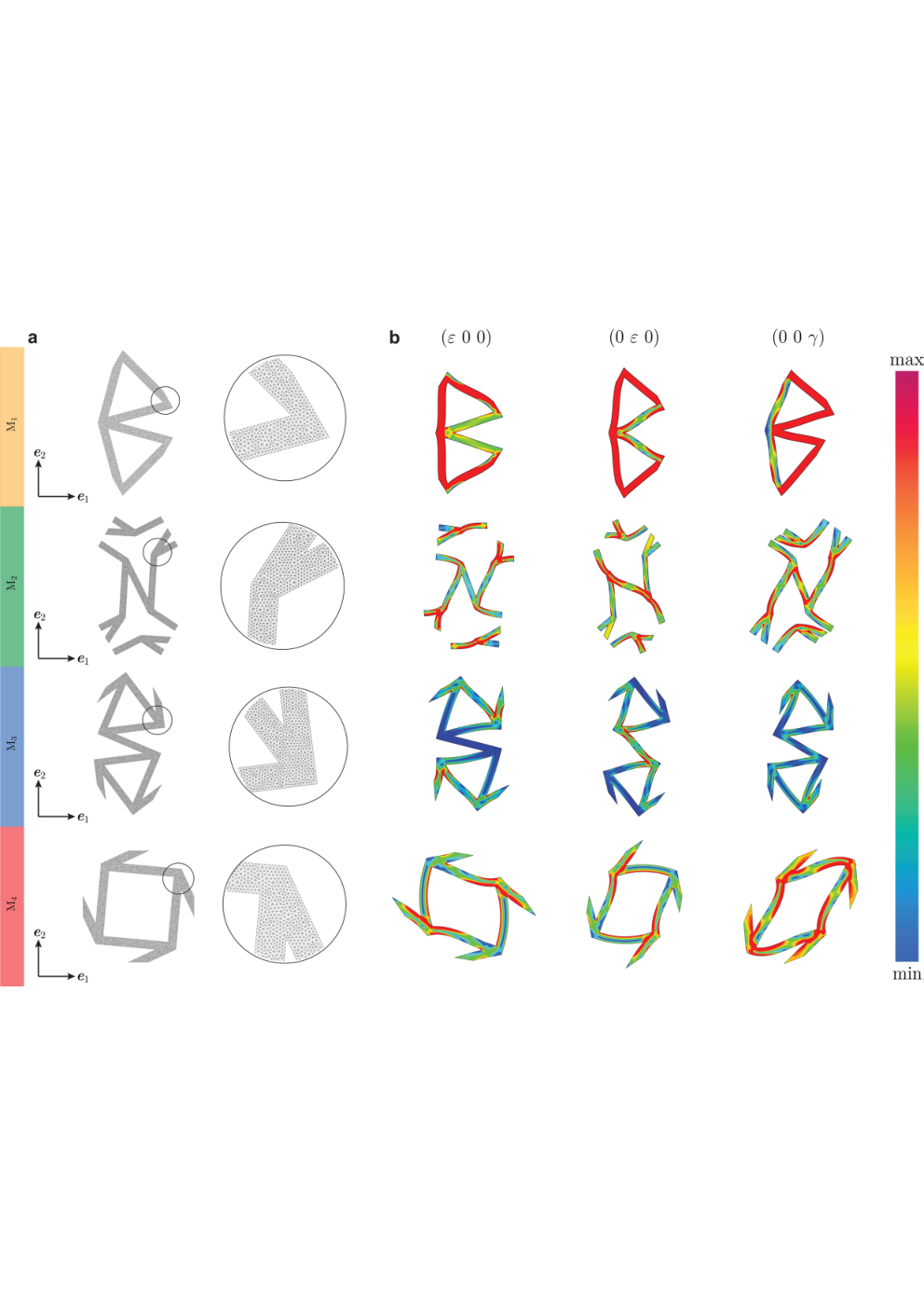
3.2 Comparison with Experimental Findings and Simulations with Finite-Sized Samples
The M1-M4 lattices were additively manufactured for and mm at finite sizes with to . The printed lattice specimens were tensile tested, and Poisson’s ratio was computed using the relative longitudinal and transverse deformations of selected control nodes on specimens, detailed in A. These and the clamping region for each finite-sized lattice are shown in Figures 5.d-h. Finite element analyses are conducted using the same finite-sized geometries and clamping conditions. Following the experiments, Young’s modulus and Poisson’s ratio were calculated using the measured tensile forces and control node kinematics.
Figures 5.a and b demonstrate the comparison of unit cell-based FE model results (broken lines), finite-sized FE model results (hollow triangles), and the experiments (filled markers with error bars and boxes). For the experiments, the markers represent the mean value of three replicates, the error bars indicate the standard deviation, and the boxes indicate the extreme values (range). A good agreement can be found between the data points for experimental results and FE models. This provides confidence in the FE model’s capabilities and the potential to translate theoretical findings to physical structures.
Each strut is printed as a single line from the nozzle; therefore, these structures represent the resolution limit achievable for this additive manufacturing process. To achieve good fidelity, it was necessary to explicitly define each movement of the nozzle. For this purpose, FullControl Gcode Designer [28] was used to create parametric designs where the unit cell size and quantity, angle, and other parameters could be easily adjusted. Since the same parametric design was used for all structures within each Mi type, any influences of the manufacturing procedure on experimental results were limited, which enabled consistent trends and good agreement with FE models. A common additive manufacturing workflow of creating a 3D CAD model and slicing it to retrospectively generate a tool-path would not achieve similar consistency. Therefore, any future work to implement these structures in practical applications should include the careful design of the tool-path. The manufacturing and tool-path design details are given in A. Another key benefit of the parametric design approach is that it would be simple to implement transitions between different angles at different positions within a structure and even to transition between the different structures M. The structures used in this paper can be parametrically adjusted and downloaded as manufacturing procedures from www.fullcontrol.xyz/#/models/1d3528.
The agreement between the periodic unit cell results and the finite-sized structural computations shows that the in-plane structural size according to Figure 5.h, with an aspect ratio of for Mi for and for M4, is sufficient to avoid size and boundary effects. Figures 5.a and b demonstrate that there is generally a good agreement between the experimentally observed and computed Poisson’s ratios and Figures 5.d, e, f, and g depict the undeformed and deformed shapes for the finite-sized lattices in finite element simulations for selected . The contour plot shows the equivalent strain. For demonstration purposes, the displacements in the direction are exaggerated by a scale factor, whereas the direction displacements are omitted. Unlike other deformed shapes, those for the anisotropic lattice M4 attain an S-like shape due to local rotations formed with chirality and the anisotropy whose major axes do not comply with the direction of the applied load for , and . As the lattice is elastomechanically anisotropic, shear is invoked upon tension. To accommodate shear under applied constraints, the planar lattice deforms into an s-shape with local rotations thanks to the chiral microstructure. Once sufficient compliance is given by increasing the aspect ratio of the effective unclamped area of the structure, then the computed Poisson’s ratios get closer to numerical results. This is inspiring in developing new lattice materials in arbitrary directions. For , the chirality is lost, and so is the S-shaped pattern with material rotations. Unlike M4, a shear deformation mode is not invoked in isotropic lattices. Either a gradual bulging or contraction is observed at the gauge section for auxetic and nonauxetic lattices under the influence of supports constraining lateral contraction. Investigating the deformation contours, the auxetic behavior in the lattices M1 and M2 are observed for , and for the former and and for the latter. For M3, a slight auxeticity is observed only for . The findings agree with the auxeticity intervals given in Figure 2.b.

3.3 Deformation Modes: An Energetic Evaluation
In energy computations, all lattices are considered rigid-jointed strut networks of beams which allow a clear separation of the deformation energy into stretching, bending, and shear parts. With no prestress, each strut is discretized with 75 two-node 2D Timoshenko beam elements. Accordingly, each node has two translational along and directions, respectively, and one rotational degree of freedom about axis, which sum up to a total of three degrees of freedom. The total potential energy per unit thickness along direction for a single strut is decomposed into stretching , bending and shear parts with
| (28) |
where the components are given as
| (29) | ||||
| (30) | ||||
| (31) |
Here, , , and , respectively, denote the width, length, and moment of inertia of the beam element. indicates the shear correction factor of the Timoshenko beam theory [83].
Considering summations over all struts in a unit cell with , , , and , one can compute the corresponding energy percentages for each deformation mechanism with
| (32) |
For three macroscopically homogeneous loading scenarios, plane strain tension, uniaxial tension, and shear, the energy percentage plots are generated and demonstrated in Figure 6.a. The reason for selecting these conditions is their use in the standard parameter identification practices for periodic unit cells. In Figure 6.a, denote the considered loading direction with . The analyses are realized for a slenderness ratio of , where shear deformation and junction effects are sufficiently suppressed. This makes two local deformation modes possible: stretching and shearing. These represent two ends of the rainbow plot as blue and red, respectively. Our simulations for also show similar results. These plots demonstrate that the dominating deformation mode is bending for all lattices except for M1. For the plane strain tension loading and as tends to the uniqueness angle , which is for M3, for M4 and for M2, a rapid transition to an axial deformation mode is observed. is the only angle the lattices M3, M4 and M2 cease to be chiral. Thus, the results show that chirality mainly invokes bending energy modes for the lattices of the same topology. Stored energy percentages over the elements are demonstrated on the exact figure for and plane strain loading along direction. The contours are given at the undeformed configuration. It is seen that all members are mainly subject to a stretching mode, regardless of their location.

As all lattices except for M4 are elastomechanically isotropic, they do not show any difference along the short edge of the plot. For M4, however, which is an anisotropic lattice, as axial deformation mode is invoked for plane strain tension and shear loads. With the elastomechanical anisotropy of the lattice, around the loading direction of , another deformation mode change is observed. Closer inspection reveals that for this is the direction of the maximum macroscopic elastic compliance. It is known that for lattices, stretching deformation modes end up giving stiffer responses, which agrees with the drawn picture. The star-polygon angle threshold seems to have no observable influence on invoking different deformation energies.
Unlike other lattices, for the non-chiral M1, a local stretching deformation mode prevails for plane strain tension and shear loading; see also Figure 4. For uniaxial tension, bending domination is observed except for the case where tends to the uniqueness angle .
These results clearly show that four factors could affect the local deformation mode of lattice systems in addition to the lattice topology, otherwise known as member connectivity. These are strut slenderness ratio, member orientations or degree of chirality, and macroscopic loading type and direction. The former two influence the load distribution among members and how the applied loads are transferred among elements. The latter two are trivial; as for a beam element, an axial load will only invoke an axial deformation mode, whereas an applied couple invokes only a pure bending mode.
Figure 6.b demonstrates versus Poisson’s ratio plot for the isotropic lattices only. The thick grey line in the background is the curve for elastically isotropic 2D materials for which . The fact that the curves for our isotropic lattices M1, M2, and M3 lie on the grey line verifies our computations. The plot also allows investigation of the intervals for which the lattices are auxetic. M1 is auxetic for most of the values, whereas M3 shows auxeticity only for a small interval of .
Material properties are mapped on the material chart relating density and Young’s modulus given in Figure 6.c, [6]. The mechanical properties of the star-polygon architectures extend the material property space for polymer materials by surpassing their conventional properties. Especially the M1 lattice architecture enables lighter but stiffer structures which are also auxetic, demonstrated by the region with dashed enclosing boundaries. In contrast, most rigid and flexible polymer foams are not auxetic [65].
4 Conclusion
This work studies the elastostatics of star-polygon tiling-based planar architectured lattice materials. The lattices are grouped into four sub-families M1, M2, M3, and M4. It is shown that many widely investigated lattice metamaterials that have been independently studied in the literature are specific variants of the presented overarching family. We conducted both numerical and experimental studies.
With an assumption of linear and infinitesimal Cauchy elasticity, numerical studies included first-order computational homogenization studies conducted over primitive periodic unit cells. This allowed computation of effective Poisson’s ratio, Young’s modulus, shear modulus, and planar bulk modulus for varying degrees of chirality and strut slenderness ratios.
Lattices are additively manufactured for selected parameters and subjected to tensile tests. The Poisson’s ratios and elasticity moduli agree well with the simulations conducted on finite-sized structures and unit cells under periodic boundary conditions.
The lattices possess attractive properties in addition to their low relative densities. As its property maps prove, the elastically isotropic M1 extends the material property space and demonstrates seemingly contrasting properties of relatively high stiffness in combination with auxeticity thanks to its axial primary deformation mode.
5 Acknowledgements
C.S. gratefully acknowledges Dr. Swantje Bargmann and the University of Wuppertal for the computational resources provided during the early developments of the work. E.S. gratefully acknowledges the funding in part from the EPSRC UK (grant number EP/R012091/1).
Appendix A Experimental methods
Polylactic acid (PLA) (ECOMAX®, 3DXTECH US) was used to print all our lattice structures. Typical elongation at break is 5.2. The glass-transition temperature is 60°C. The recommended nozzle temperature is 210°C. Tensile tests of the lattice specimens were conducted to validate the finite-element simulations. PLA bulk-material properties were obtained from the material data sheet provided by 3DXTECH®, and used as input parameters for the simulations.
A.1 Additive manufacturing of 2D lattice specimens
Fullcontrol Gcode Designer [28] was used for print path design and manufacturing Gcode generation, which facilitates parametric tool-path geometry design and process control. To minimize manufacturing defects, continuous printing paths were designed wherever possible for all lattices to avoid non-printing travel movements of the nozzle across the lattice since such movements cause defects. When an odd number of struts met at a junction (M2, M3, and M4) it was not possible to simply print to and from the junction without double-printing one line. To avoid defects in such cases, novel intricate printing strategies were designed with material retraction, varied extrusion rate, and varied printing speed. Controlled non-printing movements were designed to occur along previously printed filaments without double-printing the struts, which would normally unintentionally increase their width. These carefully designed paths also avoided defects and disturbance to previously printed filaments since the nozzle did not cross any of them laterally but tracked within their edges. An odd number of unit cells were printed in the width direction to have complete configurations with periodic patterns that started and finished on the same side of the structure, meaning each layer could be repeated, as required for additive manufacturing, without excessive non-printing nozzle movement from the end of one layer to the beginning of the next. The nozzle temperature was 210°C. The filament spool was dried at 40°C before printing. A Raise3D Pro2®(Raise 3D Technologies, USA) printer was used. The printing speed was set to 1000 mm.min, and the travelling speed was set to 6000 mm.min. The extrusion width (printed filament width) was set to 0.5mm during GCode generation, the nozzle diameter was 0.4 mm, and the layer height was 0.167mm. All lattices were printed as 3-layer single-extrusion structures to achieve 0.5-mm thick struts.
A.2 Tensile test and calculation of Poisson’s ratio
A tensile test was conducted on a universal tensile testing system (Instron®) with a load-cell of 2 kN and a constant strain rate of 0.03 min to obtain experimental material properties. For all specimens, three rows of the unit cells from both the bottom and top edges were clamped in the grips to avoid slipping or stress concentration. For Poisson’s ratio, digital image correction (DIC) was used to measure longitudinal and transverse deformation. The tests were recorded by a high-resolution 4K camera to visualize and capture corrected local deformation, as seen in Figure A.6. Four unit cell corners (junctions) evenly spaced in 2 unit cells in the center of the specimens were marked with red dots (P1-P4), as the control nodes. This enabled the measurement of local strain by measuring the average change in L3 and L4 for longitudinal-direction deformation and the average change in L1 and L2 for transverse-direction deformation simultaneously. Twelve images were selected from the camera recordings for all specimens, corresponding to engineering strains starting from 0.0001 to yielding points within the linear elastic region, facilitating tracking of the longitudinal and transverse deformation with a constant engineering strain interval.

Appendix B The Influence of Junctions - A Comparison of Continuum and Beam Idealizations
In determining the junction effects and evaluating the validity range of beam element geometric parameters, a second test was designed, which is referred to as a splitting test. This test extends an infinitely long, thin elastic spring with applied force at both ends. Considering the symmetry and translational periodicity of the problem, it is possible to concentrate on a repeating strut instead of the whole structure. Figure 8 demonstrates the problem, its continuum, beam idealizations, and assigned boundary conditions.

The numerical results are generated for two ranges of slenderness ratios. In Figure 9, Poisson’s ratio and applied splitting force for is given. The difference in Poisson’s ratios is generally smaller than in force measurements between the beam and continuum-based modeling approaches. Moreover, for the selected slenderness ratio, for the continuum and beam elements give increasingly different results.

In 10, with the increase of slenderness ratios, the difference in Poisson’s ratios seem remedied between continuum and beam-based models, whereas for force measurements, there still is a difference for and slenderness ratio of

Appendix C Tabulated Data
The tables in this section present the values of relative density and material properties at the specified values for the four families of uniform tilings having different slenderness ratios . Our computations are accomplished in two steps. In the first step, is varied in between and with the increments of , whereas in the second step, is varied in between and with the increments of . At each alpha value, is varied from to with increments of . The values of any quantity, , at , and are denoted by , and , respectively. For the chiral uniform tilings M1, M2 and M3, which show isotropy, the maximum and minimum values of any material property, , with the corresponding value these extrema appear, are denoted by and . In case of M4, these extrema are denoted by and . Here signifies the values of at which these extrema occur. Since M4 does not possess isotropy, for a specified value, Poisson’s ratio, Young’s modulus, and shear modulus are varied as a function of . Therefore, in the relevant tables, material properties have maxima and minima with respect to for a given . On the other hand, in the case of bulk modulus values of M4, this dependence vanishes. We also note that, as discussed in the paper, two different types of normalizations are used in the presentation of the results of , and which are signified by putting "" and "" over the associated quantity.
| 20 | 510 | 1200 | 270 | 300 | 355 | 400 | 633 | 1200 | 270 | 300 | |
| 30 | 360 | 800 | 187 | 200 | 247 | 267 | 482 | 800 | 187 | 200 | |
| 40 | 278 | 600 | 143 | 150 | 189 | 200 | 390 | 600 | 143 | 150 | |
| 20 | 190 | 600 | 190 | 200 | 240 | 257 | 353 | 600 | 190 | 200 | |
| 30 | 129 | 400 | 129 | 133 | 164 | 171 | 260 | 400 | 129 | 133 | |
| 40 | 97.5 | 300 | 97.5 | 100 | 124 | 129 | 207 | 300 | 97.5 | 100 | |
| 20 | 510 | 1800 | 121 | 129 | 129 | 138 | 704 | 1800 | 121 | 129 | |
| 30 | 360 | 1200 | 82.4 | 86.2 | 88.2 | 92.3 | 561 | 1200 | 82.4 | 86.2 | |
| 40 | 278 | 900 | 62.5 | 64.6 | 66.9 | 69.2 | 467 | 900 | 62.5 | 64.6 | |
| 20 | 316 | 1200 | 169 | 206 | 196 | 240 | 513 | 1200 | 169 | 206 | |
| 30 | 218 | 800 | 115 | 137 | 133 | 160 | 391 | 800 | 115 | 137 | |
| 40 | 166 | 600 | 86.8 | 103 | 101 | 120 | 317 | 600 | 86.8 | 103 |
| 20 | 0.346 | 0.338 | -0.547 | 0.346 | -0.630 | |
|---|---|---|---|---|---|---|
| 30 | 0.350 | 0.337 | -0.774 | 0.350 | -0.844 | |
| 40 | 0.349 | 0.337 | -0.870 | 0.349 | -0.919 | |
| 20 | 0.892 | 0.892 | 0.0898 | 0.892 | -0.221 | |
| 30 | 0.949 | 0.949 | 0.0405 | 0.949 | -0.406 | |
| 40 | 0.971 | 0.971 | 0.0176 | 0.971 | -0.490 | |
| 20 | 0.346 | 0.912 | 0.742 | 0.912 | 0.0309 | |
| 30 | 0.350 | 0.958 | 0.768 | 0.958 | -0.0287 | |
| 40 | 0.348 | 0.976 | 0.779 | 0.976 | -0.0594 |
| 20 | 450 | 230 | 385 | 104 | 108 | 38.3 | 495 | 309 | 75.0 | 34.6 | |
| 30 | 401 | 144 | 366 | 68.3 | 49.0 | 12.1 | 423 | 198 | 25.3 | 9.15 | |
| 40 | 380 | 105 | 357 | 50.9 | 27.1 | 5.12 | 392 | 146 | 11.6 | 3.45 | |
| 20 | 61.0 | 11.6 | 61.0 | 11.6 | 65.2 | 15.6 | 177 | 59.1 | 61.0 | 11.6 | |
| 30 | 27.6 | 3.55 | 27.6 | 3.55 | 28.7 | 4.70 | 91.2 | 21.4 | 27.6 | 3.55 | |
| 40 | 15.5 | 1.51 | 15.5 | 1.51 | 15.8 | 1.97 | 54.5 | 9.87 | 14.0 | 1.51 | |
| 20 | 450 | 230 | 44.3 | 5.36 | 38.7 | 5.00 | 547 | 381 | 17.2 | 4.32 | |
| 30 | 401 | 144 | 20.8 | 1.72 | 17.9 | 1.57 | 464 | 252 | 5.44 | 1.21 | |
| 40 | 380 | 105 | 11.9 | 0.742 | 10.1 | 0.676 | 425 | 189 | 2.42 | 0.481 |
| 20 | 167 | 85.3 | 144 | 38.9 | 119 | 42.2 | 185 | 116 | 99.8 | 38.9 | |
| 30 | 148 | 53.4 | 137 | 25.5 | 109 | 26.8 | 157 | 73.5 | 77.4 | 25.5 | |
| 40 | 141 | 39.1 | 134 | 19.0 | 104 | 19.7 | 146 | 54.2 | 66.9 | 19.0 | |
| 20 | 16.1 | 3.06 | 16.1 | 3.06 | 29.9 | 7.18 | 52.4 | 18.5 | 16.1 | 3.06 | |
| 30 | 7.07 | 0.911 | 7.07 | 0.911 | 13.8 | 2.26 | 24.8 | 5.80 | 7.07 | 0.911 | |
| 40 | 3.94 | 0.384 | 3.94 | 0.384 | 7.78 | 0.967 | 14.3 | 2.59 | 3.94 | 0.384 | |
| 20 | 167 | 85.3 | 11.6 | 1.40 | 11.1 | 1.44 | 205 | 143 | 8.13 | 1.40 | |
| 30 | 148 | 53.4 | 5.32 | 0.438 | 5.05 | 0.445 | 172 | 93.7 | 2.78 | 0.438 | |
| 40 | 141 | 39.1 | 3.01 | 0.188 | 2.84 | 0.190 | 158 | 70.2 | 1.28 | 0.188 |
| 20 | 345 | 176 | 291 | 78.5 | 34.9 | 12.4 | 373 | 233 | 23.1 | 10.7 | |
| 30 | 308 | 111 | 276 | 51.5 | 13.8 | 3.41 | 324 | 151 | 6.87 | 2.48 | |
| 40 | 292 | 80.9 | 269 | 38.4 | 7.25 | 1.37 | 301 | 112 | 3.04 | 0.898 | |
| 20 | 282 | 53.6 | 282 | 53.6 | 35.8 | 8.59 | 311 | 102 | 28.8 | 7.89 | |
| 30 | 271 | 34.9 | 271 | 34.9 | 15.0 | 2.45 | 290 | 67.4 | 10.0 | 2.02 | |
| 40 | 265 | 25.9 | 265 | 25.9 | 8.06 | 1.00 | 280 | 50.4 | 4.74 | 0.765 | |
| 20 | 345 | 176 | 253 | 30.5 | 74.9 | 9.68 | 410 | 285 | 8.98 | 2.59 | |
| 30 | 308 | 111 | 245 | 20.2 | 38.5 | 3.39 | 353 | 192 | 2.65 | 0.651 | |
| 40 | 292 | 80.9 | 242 | 15.1 | 22.8 | 1.53 | 326 | 145 | 1.14 | 0.246 |
| 20 | max | 0.938 | 0.955 | 0.799 | 0.955 | 0.573 | |
| min | 0.0751 | 0.881 | 0.146 | 0.881 | -0.820 | ||
| 30 | max | 0.973 | 0.979 | 0.814 | 0.979 | 0.570 | |
| min | 0.0496 | 0.946 | 0.147 | 0.946 | -0.929 | ||
| 40 | max | 0.985 | 0.988 | 0.818 | 0.988 | 0.566 | |
| min | 0.0371 | 0.969 | 0.148 | 0.969 | -0.962 |
| 20 | max | 562 | 64.3 | 73.0 | 609 | 55.6 | |
| min | 37.9 | 24.3 | 17.2 | 119 | 12.5 | ||
| 30 | max | 540 | 28.3 | 33.3 | 573 | 18.9 | |
| min | 15.6 | 10.8 | 7.28 | 53.0 | 4.43 | ||
| 40 | max | 529 | 15.7 | 18.8 | 555 | 8.47 | |
| min | 8.44 | 6.02 | 3.99 | 29.8 | 2.14 | ||
| 20 | max | 178 | 10.9 | 14.3 | 300 | 15.4 | |
| min | 12.0 | 4.10 | 3.37 | 59.1 | 3.23 | ||
| 30 | max | 118 | 3.24 | 4.44 | 209 | 4.62 | |
| min | 3.40 | 1.23 | 0.971 | 19.6 | 0.891 | ||
| 40 | max | 87.7 | 1.36 | 18.9 | 160 | 1.86 | |
| min | 1.40 | 0.522 | 0.403 | 8.79 | 0.359 |
| 20 | max | 261 | 17.1 | 31.9 | 270 | 127 | |
| min | 9.78 | 6.21 | 4.78 | 32.5 | 3.89 | ||
| 30 | max | 257 | 7.27 | 14.5 | 263 | 137 | |
| min | 3.95 | 2.72 | 2.01 | 13.8 | 1.42 | ||
| 40 | max | 255 | 3.99 | 8.17 | 260 | 60.8 | |
| min | 2.13 | 1.51 | 1.10 | 7.65 | 0.703 | ||
| 20 | max | 82.7 | 2.89 | 6.24 | 133 | 8.02 | |
| min | 3.09 | 1.05 | 0.936 | 16.2 | 0.931 | ||
| 30 | max | 56.0 | 0.834 | 1.93 | 95.9 | 3.61 | |
| min | 0.861 | 0.312 | 0.268 | 5.12 | 0.262 | ||
| 40 | max | 42.4 | 0.346 | 0.825 | 75.0 | 2.02 | |
| min | 0.352 | 0.131 | 0.111 | 2.25 | 0.107 |
| 20 | 304 | 271 | 42.7 | 349 | 14.8 | |
| 30 | 284 | 261 | 19.5 | 314 | 4.75 | |
| 40 | 275 | 256 | 11.0 | 297 | 2.16 | |
| 20 | 96.1 | 45.7 | 8.37 | 172 | 4.58 | |
| 30 | 61.8 | 29.9 | 2.60 | 115 | 1.15 | |
| 40 | 45.6 | 22.2 | 1.11 | 86.1 | 0.433 |
References
- ABAQUS [2019] ABAQUS. ABAQUS/Standard User’s Manual, Version 2019. Dassault Systèmes Simulia Corp, United States, 2019.
- Alderson [1999] A. Alderson. A triumph of lateral thought. Chemistry and Industry, 17:384–391, 1999.
- Alderson and Alderson [2007] A. Alderson and K. L. Alderson. Auxetic materials. Proceedings of the Institution of Mechanical Engineers, Part G: Journal of Aerospace Engineering, 221(4):565–575, 2007.
- Alderson et al. [1994] K. Alderson, A. Pickles, P. Neale, and K. Evans. Auxetic polyethylene: The effect of a negative Poisson’s ratio on hardness. Acta Metallurgica et Materialia, 42(7):2261 – 2266, 1994.
- Alderson and Evans [1993] K. L. Alderson and K. E. Evans. Strain-dependent behaviour of microporous polyethylene with a negative Poisson’s ratio. Journal of Materials Science, 28(15):4092–4098, Jan 1993.
- Ashby [2013] M. Ashby. Designing architectured materials. Scripta Materialia, 68(1):4–7, 2013. ISSN 1359-6462. doi: https://doi.org/10.1016/j.scriptamat.2012.04.033. Architectured Materials.
- Babaee et al. [2013] S. Babaee, J. Shim, J. C. Weaver, E. R. Chen, N. Patel, and K. Bertoldi. 3D soft metamaterials with negative Poisson’s ratio. Advanced Materials, 25(36):5044–5049, 2013.
- Bhate et al. [2019] D. Bhate, C. A. Penick, L. A. Ferry, and C. Lee. Classification and selection of cellular materials in mechanical design: Engineering and biomimetic approaches. Designs, 3(1), 2019.
- Cabras and Brun [2014] L. Cabras and M. Brun. Auxetic two-dimensional lattices with Poisson’s ratio arbitrarily close to -1. Proceedings of the Royal Society A: Mathematical, Physical and Engineering Sciences, 470(2172):20140538, Dec. 2014. ISSN 1364-5021, 1471-2946. doi: 10.1098/rspa.2014.0538.
- Cao et al. [2020] X. Cao, Y. Jiang, T. Zhao, P. Wang, Y. Wang, Z. Chen, Y. Li, D. Xiao, and D. Fang. Compression experiment and numerical evaluation on mechanical responses of the lattice structures with stochastic geometric defects originated from additive-manufacturing. Composites Part B: Engineering, 194:108030, Aug. 2020. ISSN 13598368. doi: 10.1016/j.compositesb.2020.108030.
- Chen [2018] H. Chen. A study of topological effects in 1D and 2D mechanical lattices. Journal of the Mechanics and Physics of Solids, page 15, 2018.
- Cherkaev and Ryvkin [2019] A. Cherkaev and M. Ryvkin. Damage propagation in 2d beam lattices: 2. Design of an isotropic fault-tolerant lattice. Arch Appl Mech, 89(3):503–519, Mar. 2019. ISSN 0939-1533, 1432-0681. doi: 10.1007/s00419-018-1428-0.
- Choi and Lakes [1995] J. B. Choi and R. S. Lakes. Nonlinear analysis of the Poisson’s ratio of negative Poisson’s ratio foams. Journal of Composite Materials, 29(1):113–128, 1995.
- Daniel et al. [2020] A. K. Daniel, R. N. Alexander, and A. Miyake. Computational universality of symmetry-protected topologically ordered cluster phases on 2D Archimedean lattices. Quantum, 4:228, Feb. 2020. ISSN 2521-327X. doi: 10.22331/q-2020-02-10-228. arXiv: 1907.13279.
- Davami et al. [2015] K. Davami, L. Zhao, E. Lu, J. Cortes, C. Lin, D. E. Lilley, P. K. Purohit, and I. Bargatin. Ultralight shape-recovering plate mechanical metamaterials. Nature Communications, page 7, 2015.
- Dong et al. [2019] Z. Dong, Y. Li, T. Zhao, W. Wu, D. Xiao, and J. Liang. Experimental and numerical studies on the compressive mechanical properties of the metallic auxetic reentrant honeycomb. Materials & Design, 182:108036, Nov. 2019. ISSN 02641275. doi: 10.1016/j.matdes.2019.108036.
- Dos Reis and Ganghoffer [2012] F. Dos Reis and J. Ganghoffer. Construction of micropolar continua from the asymptotic homogenization of beam lattices. Computers & Structures, 112-113:354–363, Dec. 2012. ISSN 00457949. doi: 10.1016/j.compstruc.2012.08.006.
- Dos Reis and Karathanasopoulos [2022] F. Dos Reis and N. Karathanasopoulos. Inverse metamaterial design combining genetic algorithms with asymptotic homogenization schemes. International Journal of Solids and Structures, 250:111702, 2022. doi: https://doi.org/10.1016/j.ijsolstr.2022.111702.
- Eddi et al. [2009] A. Eddi, A. Decelle, E. Fort, and Y. Couder. Archimedean lattices in the bound states of wave interacting particles. Europhys. Lett., 87(5):56002, Sept. 2009. ISSN 0295-5075, 1286-4854. doi: 10.1209/0295-5075/87/56002.
- Elsayed and Pasini [2010] M. S. A. Elsayed and D. Pasini. Analysis of the elastostatic specific stiffness of 2D stretching-dominated lattice materials. Mechanics of Materials, page 17, 2010.
- Estrin et al. [2021] Y. Estrin, Y. Beygelzimer, R. Kulagin, P. Gumbsch, P. Fratzl, Y. Zhu, and H. Hahn. Architecturing materials at mesoscale: some current trends. Materials Research Letters, 9(10):399–421, 2021. doi: 10.1080/21663831.2021.1961908.
- Evans and Alderson [2000] K. E. Evans and A. Alderson. Auxetic materials: Functional materials and structures from lateral thinking! Advanced Materials, 12(9):617–628, 2000.
- Evans et al. [1991] K. E. Evans, M. A. Nkansah, I. J. Hutchinson, and S. C. Rogers. Molecular network design. Nature, 353:124–125, 1991.
- Fruchart et al. [2020] M. Fruchart, Y. Zhou, and V. Vitelli. Dualities and non-Abelian mechanics. Nature, 577(7792):636–640, Jan. 2020. ISSN 0028-0836, 1476-4687. doi: 10.1038/s41586-020-1932-6.
- Gao et al. [2021] E. Gao, R. Li, S. Fang, Q. Shao, and R. H. Baughman. Bounds on the in-plane poisson’s ratios and the in-plane linear and area compressibilities for sheet crystals. Journal of the Mechanics and Physics of Solids, 152:104409, 2021. ISSN 0022-5096. doi: https://doi.org/10.1016/j.jmps.2021.104409.
- Gaspar et al. [2011] N. Gaspar, C. W. Smith, A. Alderson, J. N. Grima, and K. E. Evans. A generalised three-dimensional tethered-nodule model for auxetic materials. Journal of Materials Science, 46(2):372–384, Jan 2011.
- Gibson and Ashby [1997] L. J. Gibson and M. F. Ashby. Cellular solids: structure and properties. Cambridge Solid State Science Series. Cambridge University Press, 2 edition, 1997.
- Gleadall [2021] A. Gleadall. Fullcontrol gcode designer: Open-source software for unconstrained design in additive manufacturing. Additive Manufacturing, 46:102109. Available at www.fullcontrolgcode.com, 2021. ISSN 2214-8604. doi: https://doi.org/10.1016/j.addma.2021.102109.
- Greaves et al. [2011] G. N. Greaves, A. L. Greer, R. S. Lakes, and T. Rouxel. Poisson’s ratio and modern materials. Nature Materials, 10:823, 2011.
- Grima et al. [2001] J. N. Grima, R. Jackson, A. Alderson, and K. E. Evans. Do zeolites have negative Poisson’s ratios? Advanced Materials, 12(24):1912–1918, 2001.
- Grünbaum and Shephard [1977] B. Grünbaum and G. C. Shephard. Tilings by regular polygons. Mathematics Magazine, 50(5):227–247, 1977. doi: 10.1080/0025570X.1977.11976655.
- Gu et al. [2018] H. Gu, M. Pavier, and A. Shterenlikht. Experimental study of modulus, strength and toughness of 2D triangular lattices. International Journal of Solids and Structures, 152-153:207–216, Nov. 2018. ISSN 00207683. doi: 10.1016/j.ijsolstr.2018.06.028.
- Hou et al. [2018] S. Hou, T. Li, Z. Jia, and L. Wang. Mechanical properties of sandwich composites with 3D-printed auxetic and non-auxetic lattice cores under low velocity impact. Materials & Design, 160:1305–1321, Dec. 2018. ISSN 02641275. doi: 10.1016/j.matdes.2018.11.002.
- Hutchinson and Fleck [2006] R. Hutchinson and N. Fleck. The structural performance of the periodic truss. Journal of the Mechanics and Physics of Solids, 54(4):756–782, Apr. 2006. ISSN 00225096. doi: 10.1016/j.jmps.2005.10.008.
- Jeong et al. [2016] G. S. Jeong, D. Y. No, J. Lee, J. Yoon, S. Chung, and S.-H. Lee. Viscoelastic lithography for fabricating self-organizing soft micro-honeycomb structures with ultra-high aspect ratios. Nat Commun, 7(1):11269, Sept. 2016. ISSN 2041-1723. doi: 10.1038/ncomms11269.
- Jiang et al. [2022] H. Jiang, H. Ziegler, Z. Zhang, H. Zhang, L. Le Barbenchon, S. Atre, and Y. Chen. 3D printed tubular lattice metamaterials for mechanically robust stents. Composites Part B: Engineering, 236:109809, May 2022. ISSN 13598368. doi: 10.1016/j.compositesb.2022.109809.
- Jiang et al. [2018] W. Jiang, L. Yan, H. Ma, Y. Fan, J. Wang, M. Feng, and S. Qu. Electromagnetic wave absorption and compressive behavior of a three-dimensional metamaterial absorber based on 3D printed honeycomb. Sci Rep, 8(1):4817, Dec. 2018. ISSN 2045-2322. doi: 10.1038/s41598-018-23286-6.
- Jin et al. [2019] N. Jin, F. Wang, Y. Wang, B. Zhang, H. Cheng, and H. Zhang. Effect of structural parameters on mechanical properties of Pyramidal Kagome lattice material under impact loading. International Journal of Impact Engineering, 132:103313, Oct. 2019. ISSN 0734-743X. doi: 10.1016/j.ijimpeng.2019.06.002.
- Jones [1999] R. M. Jones. Mechanics of Composite Materials. Materials Science and Engineering Series. Taylor and Francis, 2nd ed edition, 1999.
- Karathanasopoulos and Rodopoulos [2022] N. Karathanasopoulos and D. Rodopoulos. Enhanced Cellular Materials through Multiscale, Variable-Section Inner Designs: Mechanical Attributes and Neural Network Modeling. Materials (Basel), 15(10):3581, 2022. doi: https://doi.org/10.3390/ma15103581.
- Karathanasopoulos et al. [2018] N. Karathanasopoulos, F. Dos Reis, H. Reda, and J.-F. Ganghoffer. Computing the effective bulk and normal to shear properties of common two-dimensional architectured materials. Computational Materials Science, 154:284–294, 2018. ISSN 0927-0256. doi: https://doi.org/10.1016/j.commatsci.2018.07.044.
- Karathanasopoulos et al. [2020] N. Karathanasopoulos, F. Dos Reis, P. Hadjidoukas, and J. Ganghoffer. Latticemech: A discrete mechanics code to compute the effective static properties of 2d metamaterial structures. SoftwareX, 11:100446, 2020. ISSN 2352-7110. doi: https://doi.org/10.1016/j.softx.2020.100446.
- Kim et al. [2019] Y. Kim, Y. Kim, F. Libonati, and S. Ryu. Designing tough isotropic structural composite using computation, 3D printing and testing. Composites Part B: Engineering, 167:736–745, June 2019. ISSN 13598368. doi: 10.1016/j.compositesb.2019.03.039.
- Kolken et al. [2018] H. M. A. Kolken, S. Janbaz, S. M. A. Leeflang, K. Lietaert, H. H. Weinans, and A. A. Zadpoor. Rationally designed meta-implants: a combination of auxetic and conventional meta-biomaterials. Materials Horizons, 5(1):28–35, 2018.
- Kouznetsova et al. [2001] V. Kouznetsova, W. A. M. Brekelmans, and F. P. T. Baaijens. An approach to micro-macro modeling of heterogeneous materials. Computational Mechanics, 27(1):37–48, Jan 2001.
- Kuang et al. [2005] W. Kuang, Z. Hou, Y. Liu, and H. Li. The bandgap of a photonic crystal with triangular dielectric rods in a honeycomb lattice. Journal of Optics A: Pure and Applied Optics, 7(10):525–528, sep 2005. doi: 10.1088/1464-4258/7/10/001.
- Lakes [1987] R. Lakes. Foam structures with a negative Poisson’s ratio. Science, 235(4792):1038–1040, 1987.
- Lei et al. [2020] Z. Lei, L. Liu, H. Zhao, F. Liang, S. Chang, L. Li, Y. Zhang, Z. Lin, J. Kröger, and Y. Lei. Nanoelectrode design from microminiaturized honeycomb monolith with ultrathin and stiff nanoscaffold for high-energy micro-supercapacitors. Nat Commun, 11(1):299, Dec. 2020. ISSN 2041-1723. doi: 10.1038/s41467-019-14170-6.
- Li et al. [2019] R. Li, Q. Shao, E. Gao, and Z. Liu. Elastic anisotropy measure for two-dimensional crystals. Extreme Mechanics Letters, 34:100615, 12 2019. doi: 10.1016/j.eml.2019.100615.
- Li et al. [2018] T. Li, Y. Chen, X. Hu, Y. Li, and L. Wang. Exploiting negative Poisson’s ratio to design 3D-printed composites with enhanced mechanical properties. Materials & Design, 142:247 – 258, 2018.
- Liarte [2020] D. B. Liarte. Multifunctional twisted kagome lattices: Tuning by pruning mechanical metamaterials. Physical Review E, page 10, 2020.
- Masters and Evans [1996] I. Masters and K. Evans. Models for the elastic deformation of honeycombs. Composite Structures, 35(4):403 – 422, 1996.
- McHale et al. [2020] C. McHale, R. Telford, and P. M. Weaver. Morphing lattice boom for space applications. Composites Part B: Engineering, 202:108441, Dec. 2020. ISSN 13598368. doi: 10.1016/j.compositesb.2020.108441.
- Mizzi et al. [2018] L. Mizzi, E. M. Mahdi, K. Titov, R. Gatt, D. Attard, K. E. Evans, J. N. Grima, and J.-C. Tan. Mechanical metamaterials with star-shaped pores exhibiting negative and zero Poisson’s ratio. Materials and Design, page 10, 2018.
- Mousanezhad et al. [2015] D. Mousanezhad, S. Babaee, H. Ebrahimi, R. Ghosh, A. S. Hamouda, K. Bertoldi, and A. Vaziri. Hierarchical honeycomb auxetic metamaterials. Scientific Reports, 5(1):18306, Dec. 2015. ISSN 2045-2322. doi: 10.1038/srep18306. Number: 1 Publisher: Nature Publishing Group.
- Nelissen et al. [2019] W. Nelissen, C. Ayas, and C. Tekog̃lu. 2D lattice material architectures for actuation. Journal of the Mechanics and Physics of Solids, 124:83–101, Mar. 2019. ISSN 00225096. doi: 10.1016/j.jmps.2018.09.035.
- Neumann [1885] F. E. Neumann. Vorlesungen über mathematische Physik: Vorlesungen über die Theorie der Elasticität der festen Körper und des Lichtäthers. B. G. Teubner, Leipzig, 1885.
- Niu and Wang [2016] B. Niu and B. Wang. Directional mechanical properties and wave propagation directionality of kagome honeycomb structures. European Journal of Mechanics - A/Solids, 57:45–58, 2016. ISSN 0997-7538. doi: https://doi.org/10.1016/j.euromechsol.2015.12.003.
- Nkansah et al. [1994] M. A. Nkansah, K. E. Evans, and I. J. Hutchinson. Modelling the mechanical properties of an auxetic molecular network. Modelling and Simulation in Materials Science and Engineering, 2(3):337, 1994.
- Nye [1985] J. F. Nye. Physical Properties of Crystals. Clarendon Press, Oxford, 1985.
- Ostoja-Starzewski [2002] M. Ostoja-Starzewski. Lattice models in micromechanics. Applied Mechanics Reviews, 55(1):35–60, 01 2002. ISSN 0003-6900. doi: 10.1115/1.1432990.
- Phani et al. [2006] A. S. Phani, J. Woodhouse, and N. A. Fleck. Wave propagation in two-dimensional periodic lattices. The Journal of the Acoustical Society of America, 119(4):1995–2005, 2006. doi: 10.1121/1.2179748.
- Podestá et al. [2019] J. Podestá, C. Méndez, S. Toro, and A. Huespe. Symmetry considerations for topology design in the elastic inverse homogenization problem. Journal of the Mechanics and Physics of Solids, 128:54–78, July 2019. ISSN 00225096. doi: 10.1016/j.jmps.2019.03.018.
- Pronk et al. [2017] T. Pronk, C. Ayas, and C. Tekog̃lu. A quest for 2D lattice materials for actuation. Journal of the Mechanics and Physics of Solids, 105:199–216, Aug. 2017. ISSN 00225096. doi: 10.1016/j.jmps.2017.05.007.
- Rinde [1970] J. A. Rinde. Poisson’s ratio for rigid plastic foams. Journal of Applied Polymer Science, 14(8):1913–1926, 1970. doi: https://doi.org/10.1002/app.1970.070140801.
- Rossi et al. [2021] N. Rossi, J. M. Podestá, F. Bre, C. G. Méndez, and A. E. Huespe. A microarchitecture design methodology to achieve extreme isotropic elastic properties of composites based on crystal symmetries. Structural and Multidisciplinary Optimization, 63(5):2459–2472, May 2021. ISSN 1615-147X, 1615-1488. doi: 10.1007/s00158-020-02823-w.
- Schaedler and Carter [2016] T. A. Schaedler and W. B. Carter. Architected cellular materials. Annual Review of Materials Research, 46(1):187–210, 2016. doi: 10.1146/annurev-matsci-070115-031624.
- Seiler et al. [2019a] P. Seiler, H. Tankasala, and N. Fleck. Creep failure of honeycombs made by rapid prototyping. Acta Materialia, 178:122–134, Oct. 2019a. ISSN 13596454. doi: 10.1016/j.actamat.2019.07.054.
- Seiler et al. [2019b] P. Seiler, H. Tankasala, and N. Fleck. The role of defects in dictating the strength of brittle honeycombs made by rapid prototyping. Acta Materialia, 171:190–200, June 2019b. ISSN 13596454. doi: 10.1016/j.actamat.2019.03.036.
- Shabanpour [2020] J. Shabanpour. Reconfigurable honeycomb metamaterial absorber having incident angular stability. Scientific Reports, page 8, 2020.
- Shimada [2015] T. Shimada. Hierarchical ferroelectric and ferrotoroidic polarizations coexistent in nano-metamaterials. Scientific Reports, page 8, 2015.
- Smeets et al. [2021] B. J. Smeets, E. M. Fagan, K. Matthews, R. Telford, B. R. Murray, L. Pavlov, B. Weafer, P. Meier, and J. Goggins. Structural testing of a shear web attachment point on a composite lattice cylinder for aerospace applications. Composites Part B: Engineering, 212:108691, May 2021. ISSN 13598368. doi: 10.1016/j.compositesb.2021.108691.
- Song and Li [2017] Z.-G. Song and F.-M. Li. Flutter and buckling characteristics and active control of sandwich panels with triangular lattice core in supersonic airflow. Composites Part B: Engineering, 108:334–344, Jan. 2017. ISSN 13598368. doi: 10.1016/j.compositesb.2016.10.013.
- Soyarslan et al. [2018] C. Soyarslan, H. Argeso, and S. Bargmann. Skeletonization-based beam finite element models for stochastic bicontinuous materials: Application to simulations of nanoporous gold. Journal of Materials Research, 33(20):3371–3382, 2018. doi: 10.1557/jmr.2018.244.
- Soyarslan et al. [2019] C. Soyarslan, V. Blümer, and S. Bargmann. Tunable auxeticity and elastomechanical symmetry in a class of very low density core-shell cubic crystals. Acta Materialia, 177:280–292, 2019. ISSN 1359-6454. doi: https://doi.org/10.1016/j.actamat.2019.07.015.
- Tancogne-Dejean et al. [2019] T. Tancogne-Dejean, N. Karathanasopoulos, and D. Mohr. Stiffness and Strength of Hexachiral Honeycomb-Like Metamaterials. Journal of Applied Mechanics, 86(11):111010, Nov. 2019. ISSN 0021-8936, 1528-9036. doi: 10.1115/1.4044494.
- Tankasala et al. [2017] H. Tankasala, V. Deshpande, and N. Fleck. Tensile response of elastoplastic lattices at finite strain. Journal of the Mechanics and Physics of Solids, 109:307–330, Dec. 2017. ISSN 00225096. doi: 10.1016/j.jmps.2017.02.002.
- Tankasala and Fleck [2020] H. C. Tankasala and N. A. Fleck. The crack growth resistance of an elastoplastic lattice. International Journal of Solids and Structures, 188-189:233–243, Apr. 2020. ISSN 00207683. doi: 10.1016/j.ijsolstr.2019.10.007.
- Theocaris et al. [1997] P. S. Theocaris, G. E. Stavroulakis, and P. D. Panagiotopoulos. Negative Poisson’s ratios in composites with star-shaped inclusions: a numerical homogenization approach. Archive of Applied Mechanics (Ingenieur Archiv), 67(4):274–286, Apr. 1997. ISSN 0939-1533, 1432-0681. doi: 10.1007/s004190050117.
- Ting and Chen [2005] T. C. T. Ting and T. Chen. Poisson’s ratio for anisotropic elastic materials can have no bounds. The Quarterly Journal of Mechanics and Applied Mathematics, 58(1):73–82, 2005.
- Vigliotti and Pasini [2013] A. Vigliotti and D. Pasini. Mechanical properties of hierarchical lattices. Mechanics of Materials, 62:32–43, Aug. 2013. ISSN 01676636. doi: 10.1016/j.mechmat.2013.03.003.
- Vigliotti et al. [2014] A. Vigliotti, V. S. Deshpande, and D. Pasini. Non linear constitutive models for lattice materials. Journal of the Mechanics and Physics of Solids, 64:44–60, 2014. ISSN 0022-5096. doi: https://doi.org/10.1016/j.jmps.2013.10.015.
- Weaver and Jonhston [1987] W. Weaver and P. R. Jonhston. Structural Dynamics by Finite Elements. Prentice-Hall, Englewood Cliffs, NJ, 1987.
- Wu et al. [2015] G. Wu, Y. Cho, I.-S. Choi, D. Ge, J. Li, H. N. Han, T. Lubensky, and S. Yang. Directing the Deformation Paths of Soft Metamaterials with Prescribed Asymmetric Units. Adv. Mater., page 7, 2015.
- Xiang [2018] L. Xiang. Yield surfaces of periodic honeycombs with tunable Poisson’s ratio. International Journal of Mechanical Sciences, page 13, 2018.
- Xiao et al. [2020] R. Xiao, X. Feng, R. Fan, S. Chen, J. Song, L. Gao, and Y. Lu. 3D printing of titanium-coated gradient composite lattices for lightweight mandibular prosthesis. Composites Part B: Engineering, 193:108057, July 2020. ISSN 13598368. doi: 10.1016/j.compositesb.2020.108057.
- Yera et al. [2020] R. Yera, N. Rossi, C. Méndez, and A. Huespe. Topology design of 2D and 3D elastic material microarchitectures with crystal symmetries displaying isotropic properties close to their theoretical limits. Applied Materials Today, 18:100456, Mar. 2020. ISSN 23529407. doi: 10.1016/j.apmt.2019.100456.
- Yera et al. [2022] R. Yera, L. Forzani, C. G. Méndez, and A. E. Huespe. A topology optimization algorithm based on topological derivative and level-set function for designing phononic crystals. Engineering Computations, 39(1):354–379, Feb. 2022. ISSN 0264-4401. doi: 10.1108/EC-06-2021-0352.
- Yuan et al. [2018] C. Yuan, X. Mu, C. K. Dunn, J. Haidar, T. Wang, and H. J. Qi. Thermomechanically triggered two-stage pattern switching of 2d lattices for adaptive structures. Adv. Funct. Mater., page 9, 2018.
- Zhang and Mao [2018] L. Zhang and X. Mao. Fracturing of topological maxwell lattices. New J. Phys., 20(6):063034, June 2018. ISSN 1367-2630. doi: 10.1088/1367-2630/aac765.
- Zhang et al. [2008] Y. Zhang, X. Qiu, and D. Fang. Mechanical Properties of two novel planar lattice structures. International Journal of Solids and Structures, 45(13):3751–3768, June 2008. ISSN 00207683. doi: 10.1016/j.ijsolstr.2007.10.005.
- Zheng et al. [2013] Q. Zheng, H. Fan, J. Liu, Y. Ma, and L. Yang. Hierarchical lattice composites for electromagnetic and mechanical energy absorptions. Composites Part B: Engineering, 53:152–158, Oct. 2013. ISSN 13598368. doi: 10.1016/j.compositesb.2013.04.057.
- Zhu et al. [2019] X. Zhu, L. Xu, X. Liu, J. Xu, P. Hu, and Z.-D. Ma. Theoretical prediction of mechanical properties of 3D printed Kagome honeycombs and its experimental evaluation. Proceedings of the Institution of Mechanical Engineers, Part C: Journal of Mechanical Engineering Science, 233(18):6559–6576, Sept. 2019. ISSN 0954-4062, 2041-2983. doi: 10.1177/0954406219860538.