跳到论文正文
W Papers独立论文阅读器 arXiv:2209.09822 论文正文 计算阅读时间 · 0%
引用这篇论文根据当前论文元数据生成,正式投稿前建议核对。


License: arXiv.org perpetual non-exclusive license
arXiv:2209.09822v1 [math.NA] 20 Sep 2022

Polynomial approximation of derivatives by the constrained mock-Chebyshev least squares operator

F. Dell’Accio Affiliation: Department of Mathematics and Computer Science, University of Calabria, Rende (CS), Italy    F. Nudo Affiliation: Department of Mathematics and Computer Science, University of Calabria, Rende (CS), Italy
Abstract

The constrained mock-Chebyshev least squares operator is a linear approximation operator based on an equispaced grid of points. Like other polynomial or rational approximation methods, it was recently introduced in order to defeat the Runge phenomenon that occurs when using polynomial interpolation on large sets of equally spaced points. The idea is to improve the mock-Chebyshev subset interpolation, where the considered function ff is interpolated only on a proper subset of the uniform grid, formed by nodes that mimic the behavior of Chebyshev–Lobatto nodes. In the mock-Chebyshev subset interpolation all remaining nodes are discarded, while in the constrained mock-Chebyshev least squares interpolation they are used in a simultaneous regression, with the aim to further improving the accuracy of the approximation provided by the mock-Chebyshev subset interpolation. The goal of this paper is two-fold. We discuss some theoretical aspects of the constrained mock-Chebyshev least squares operator and present new results. In particular, we introduce explicit representations of the error and its derivatives. Moreover, for a sufficiently smooth function ff in [−1,1][-1,1], we present a method for approximating the successive derivatives of ff at a point x∈[−1,1]x\in[-1,1], based on the constrained mock-Chebyshev least squares operator and provide estimates for these approximations. Numerical tests demonstrate the effectiveness of the proposed method.

1 Introduction

Let Xn={x0,…,xn}X_{n}=\{x_{0},\dots,x_{n}\} be the set of n+1n+1 equispaced nodes in [−1,1][-1,1], that is

xi=−1+2ni,i=0,…,n.x_{i}=-1+\frac{2}{n}i,\quad i=0,\dots,n.

In order to define the constrained mock-Chebyshev least squares linear operator, some settings are needed. We set

m=⌊π​n2⌋,p=⌊π2​n6⌋,m=\left\lfloor\pi\sqrt{\frac{n}{2}}\right\rfloor,\quad p=\left\lfloor\frac{\pi}{\sqrt{2}}\sqrt{\frac{{{n}}}{{{6}}}}\right\rfloor,

and we consider a basis ℬ={u0​(x),…,ur​(x)}\mathcal{B}=\{u_{0}(x),\dots,u_{r}(x)\} of the polynomial space Πr\Pi_{r}, constituted by polynomials of degree less than or equal to r=m+p+1r=m+p+1. We denote by Xm′={xk′}k=0mX^{\prime}_{m}=\{x^{\prime}_{k}\}_{k=0}^{m} the subset of mock-Chebyshev nodes [1, 10, 11], that is the nodes of the uniform grid XnX_{n} which best mimic the behavior of the well known Chebyshev–Lobatto nodes and by Xn−m′′=Xn∖Xm′X^{\prime\prime}_{n-m}=X_{n}\setminus X^{\prime}_{m} the relative complement of Xm′X^{\prime}_{m} with respect to XnX_{n}. In [5] it is proven that, when nn is sufficiently large, we can approximate an equispaced grid of q=⌊n6⌋q=\left\lfloor\frac{n}{6}\right\rfloor internal nodes of [−1,1][-1,1] with nodes which belong to Xn−m′′X^{\prime\prime}_{n-m}. We denote this grid by X~n−m′′,\tilde{X}^{\prime\prime}_{n-m}, and by Xp′′′={xk′′′}k=0pX^{\prime\prime\prime}_{p}=\{x^{\prime\prime\prime}_{k}\}_{k=0}^{p} the mock-Chebyshev subset of X~n−m′′\tilde{X}^{\prime\prime}_{n-m}. We suppose to have reordered the set XnX_{n} so that its first m+1m+1 points are those of Xm′X^{\prime}_{m}. We suppose also that the first m+1m+1 elements of the basis ℬ\mathcal{B} span the polynomial space Πm\Pi_{m}. We define the constrained mock-Chebyshev least squares linear operator as follows

P^r,n:C⁡([−1,1])\displaystyle\hat{P}_{r,n}:C([-1,1]) →\displaystyle\rightarrow C⁡([−1,1])\displaystyle C([-1,1])
f⁡(x)\displaystyle f(x) ↦\displaystyle\mapsto P^r,n​[f]​(x)=∑i=0ra^i​ui​(x),x∈[−1,1],\displaystyle\hat{P}_{r,n}[f](x)=\sum_{i=0}^{r}\hat{a}_{i}u_{i}(x),\qquad x\in[-1,1],

where 𝒂^=[a^0,a^1,…,a^r]T\hat{\boldsymbol{a}}=[\hat{a}_{0},\hat{a}_{1},\dots,\hat{a}_{r}]^{T} is the solution of the KKT linear equations [2]

[2​VT​VCTC0]​[𝒂^𝒛^]=[2​VT​𝒃𝒅].\begin{bmatrix}2V^{T}V&C^{T}\\ C&0\\ \end{bmatrix}\begin{bmatrix}\hat{\boldsymbol{a}}\\ \hat{\boldsymbol{z}}\\ \end{bmatrix}=\begin{bmatrix}2V^{T}\boldsymbol{b}\\ \boldsymbol{d}\\ \end{bmatrix}. (1)

In the equation (1) the matrices VV and CC are defined as follows

V=[uj​(xi)]i=0,…,nj=0,…,r,C=[uj​(xi)]i=0,…,mj=0,…,r,V=[u_{j}(x_{i})]_{\begin{subarray}{c}i=0,\dots,n\\ j=0,\dots,r\end{subarray}},\qquad C=[u_{j}(x_{i})]_{\begin{subarray}{c}i=0,\dots,m\\ j=0,\dots,r\end{subarray}},

𝒃=[f⁡(x0),…,f⁡(xn)]T\boldsymbol{b}=[f(x_{0}),\dots,f(x_{n})]^{T}, 𝒅=[f⁡(x0),…,f⁡(xm)]T\boldsymbol{d}=[f(x_{0}),\dots,f(x_{m})]^{T}, and 𝒛^=[z1^,…,z^m+1]T\hat{\boldsymbol{z}}=[\hat{z_{1}},\dots,\hat{z}_{m+1}]^{T} is the Lagrange multipliers vector. The matrix

M=[2​VT​VCTC0]M=\begin{bmatrix}2V^{T}V&C^{T}\\ C&0\\ \end{bmatrix} (2)

is non singular [7] and is called KKT matrix, in honor to W. Karush, H.W. Kuhn and A. Tucker [2, Chapter 16]. The operator P^r,n\hat{P}_{r,n} satisfies the following properties:

  • i)

    P^r,n\hat{P}_{r,n} is a linear operator [6], that is

    P^r,n​[λ​f+μ​g]=λ​P^r,n​[f]+μ​P^r,n​[g],f,g∈C⁡([−1,1]),λ,μ∈ℝ;\hat{P}_{r,n}\left[\lambda f+\mu g\right]=\lambda\hat{P}_{r,n}[f]+\mu\hat{P}_{r,n}[g],\quad f,g\in C([-1,1]),\,\quad\lambda,\mu\in\mathbb{R}; (3)
  • ii)

    the range of P^r,n\hat{P}_{r,n} is Πr​([−1,1])\Pi_{r}([-1,1]);

  • iii)

    P^r,n\hat{P}_{r,n} reproduces polynomials of degree ≤r\leq r [5], that is

    P^r,n​[q]=q, for each ​q∈Πr;\hat{P}_{r,n}[q]=q,\quad\text{ for each }q\in\Pi_{r}; (4)
  • iv)

    P^r,n\hat{P}_{r,n} is idempotent, that is

    P^r,n2=P^r,n;\hat{P}_{r,n}^{2}=\hat{P}_{r,n};
  • v)

    P^r,n​[f]\hat{P}_{r,n}[f] is completely determined by the evaluations of ff on the grid XnX_{n}, in particular

    P^r,n​[f]=P^r,n​[Pn​[f]], for each ​f∈C⁡([−1,1]),\hat{P}_{r,n}[f]=\hat{P}_{r,n}\left[P_{n}[f]\right],\quad\text{ for each }\,f\in C([-1,1]), (5)

    where

    Pn​[f]​(x)=∑i=0nf⁡(xi)​ℓi​(x),x∈[−1,1],P_{n}[f](x)=\sum_{i=0}^{n}f(x_{i})\ell_{i}(x),\quad x\in[-1,1],

    and

    ℓi(x)=∏j=0j≠inx−xjxi−xj,i=0,…,n,x∈[−1,1].\ell_{i}(x)=\prod\limits_{\begin{subarray}{c}j=0\\ j\neq i\end{subarray}}^{n}\frac{x-x_{j}}{x_{i}-x_{j}},\quad i=0,\dots,n,\quad x\in[-1,1].
  • vi)

    P^r,n\hat{P}_{r,n} interpolates the function ff at the mock-Chebyshev subset of nodes, that is

    P^r,n[f](xi′)=f(xi′),i=0,…,m.\hat{P}_{r,n}[f](x^{\prime}_{i})=f(x^{\prime}_{i}),\quad i=0,\dots,m.

The constrained mock-Chebyshev least squares operator has been very recently generalized to the bivariate case [7] and used to introduce accurate and stable quadrature formulas on equispaced nodes [6]. Despite some bound in uniform norm of the error of approximation

R^r,n​[f]​(x):=f⁡(x)−P^r,n​[f]​(x),x∈[−1,1],\hat{R}_{r,n}[f](x):=f(x)-\hat{P}_{r,n}[f](x),\quad x\in[-1,1], (6)

was already discussed in [5], any explicit representation of the error R^r,n​[f]\hat{R}_{r,n}[f] has not been given yet. In this paper we face this problem and provide a pointwise representation of the error which takes into account the peculiarity of P^r,n​[f]\hat{P}_{r,n}[f] of being a mixed interpolation-regression polynomial. Starting from this representation, bounds of the error (6) in uniform norm will be given through the operator norm of P^r,n\hat{P}_{r,n} and the error of best uniform approximation by polynomials of degree less than or equal to rr. For a sufficiently smooth function ff in [−1,1][-1,1], we obtain explicit representations of the derivative of the error (6) by differentiation and bounds in uniform norm by applying the Markov Theorem [14]. As an application, we introduce a new differentiation method for approximating the successive derivatives of a sufficiently smooth function ff in [−1,1][-1,1] based on the constrained mock-Chebyshev least squares operator. Furthermore, we prove an iterative relationship between the coefficients of P^r,n(ν)\hat{P}^{(\nu)}_{r,n} and those of P^r,n(ν−1)\hat{P}^{(\nu-1)}_{r,n}, when they are expressed in the Chebyshev polynomial basis of first kind.

The paper is organized as follows. In Section 2 we discuss some theoretical aspects of the constrained mock-Chebyshev least squares operator. We present a theoretical bound for the norm of this operator and we introduce explicit representations of the error and its derivatives. Basing on this operator, in Section 3, we present a differentiation method for approximating the successive derivatives of a sufficiently smooth function ff at any point x∈[−1,1]x\in[-1,1]. This method provides a global polynomial approximations of the successive derivatives of ff. The accuracy of this method is proved by several numerical examples, presented in Section 4.

2 Constrained mock-Chebyshev least squares linear operator: theoretical aspects

In this Section, we provide pointwise representations of the error (6) in terms of finite differences of the function f∈C⁡([−1,1])f\in C([-1,1]) or its appropriate derivative, if ff is sufficiently smooth, and give related bounds in uniform norm. If ff is sufficiently smooth in [−1,1][-1,1] we provide explicit representations for the successive derivatives of the error (6) and give related bounds in uniform norm. To this aim, some preliminary results are needed. First of all, we give a bound for the norm of the operator P^r,n\hat{P}_{r,n},

‖P^r,n‖:=supf∈C⁡([−1,1])‖f‖∞≤1‖P^r,n​[f]‖∞.\left\lVert\hat{P}_{r,n}\right\rVert:=\sup\limits_{\begin{subarray}{c}f\in C([-1,1])\\ \left\lVert f\right\rVert_{\infty}\leq 1\end{subarray}}\left\lVert\hat{P}_{r,n}[f]\right\rVert_{\infty}. (7)
Theorem 1.

The constrained mock-Chebyshev least squares operator is bounded. In particular

‖P^r,n‖≤C⁡(2​(r+1)​κ​(M)+(m+1)​‖M−1‖1),\left\lVert\hat{P}_{r,n}\right\rVert\leq C\left(2(r+1)\kappa(M)+(m+1)\left\lVert M^{-1}\right\rVert_{1}\right), (8)

where

C:=maxj=0,…,r⁡‖uj‖∞,κ⁡(M)=‖M‖1​∥M−1∥1.C:=\max_{j=0,\dots,r}\left\lVert u_{j}\right\rVert_{\infty},\qquad\kappa(M)=\left\lVert M\right\rVert_{1}\lVert M^{-1}\rVert_{1}. (9)
Proof.

Let f∈C⁡([−1,1])f\in C([-1,1]) be a continuous function such that ‖f‖∞≤1\left\lVert f\right\rVert_{\infty}\leq 1. By using the triangular inequality we get

|P^r,n​[f]​(x)|=|∑i=0ra^i​ui​(x)|≤∑i=0r|a^i|​|ui​(x)|,x∈[−1,1].\left\lvert\hat{P}_{r,n}[f](x)\right\rvert=\left\lvert\sum_{i=0}^{r}\hat{a}_{i}u_{i}(x)\right\rvert\leq\sum_{i=0}^{r}\left\lvert\hat{a}_{i}\right\rvert\left\lvert u_{i}(x)\right\rvert,\quad x\in[-1,1]. (10)

From (10), by passing to the supremum with respect to x∈[−1,1]x\in[-1,1], by the setting (9) we get

‖P^r,n​[f]‖∞≤C​∑i=0r|a^i|=C​‖𝒂^‖1.\left\lVert\hat{P}_{r,n}[f]\right\rVert_{\infty}\leq C\sum_{i=0}^{r}\left\lvert\hat{a}_{i}\right\rvert=C\left\lVert\hat{\boldsymbol{a}}\right\rVert_{1}. (11)

We bound the 11-norm of the coefficients vector 𝒂^\hat{\boldsymbol{a}} as follows. Since the KKT matrix (2) is not singular, from the linear system (1) we get

‖𝒂^‖1≤‖[𝒂^𝒛^]‖1\displaystyle\left\lVert\hat{\boldsymbol{a}}\right\rVert_{1}\leq\left\lVert\begin{bmatrix}\hat{\boldsymbol{a}}\\ \hat{\boldsymbol{z}}\\ \end{bmatrix}\right\rVert_{1} ≤\displaystyle\leq ‖M−1‖1​‖[2​VT​𝒃𝒅]‖1\displaystyle\left\lVert M^{-1}\right\rVert_{1}\left\lVert\begin{bmatrix}2V^{T}\boldsymbol{b}\\ \boldsymbol{d}\\ \end{bmatrix}\right\|_{1}
=\displaystyle= ‖M−1‖1​(2​∑j=0r|∑i=0nuj​(xi)​f​(xi)|+∑j=0m|f⁡(xj)|)\displaystyle\left\lVert M^{-1}\right\rVert_{1}\left(2\sum_{j=0}^{r}\left\lvert\sum_{i=0}^{n}u_{j}(x_{i})f(x_{i})\right\rvert+\sum_{j=0}^{m}\left\lvert f(x_{j})\right\rvert\right)
≤\displaystyle\leq ‖M−1‖1​(2​∑j=0r∑i=0n|uj​(xi)|+m+1)\displaystyle\left\lVert M^{-1}\right\rVert_{1}\left(2\sum_{j=0}^{r}\sum_{i=0}^{n}\left\lvert u_{j}(x_{i})\right\rvert+m+1\right)
≤\displaystyle\leq ‖M−1‖1​(2​‖M‖1​(r+1)+m+1).\displaystyle\left\lVert M^{-1}\right\rVert_{1}\left(2\left\lVert M\right\rVert_{1}(r+1)+m+1\right).

Therefore

‖𝒂^‖1≤2​(r+1)​κ​(M)+(m+1)​‖M−1‖1.\left\lVert\hat{\boldsymbol{a}}\right\rVert_{1}\leq 2(r+1)\kappa(M)+(m+1)\left\lVert M^{-1}\right\rVert_{1}. (12)

Finally, by using the bound (12) in (11), we get

‖P^r,n​[f]‖∞≤C⁡(2​(r+1)​κ​(M)+(m+1)​‖M−1‖1).\left\lVert\hat{P}_{r,n}[f]\right\rVert_{\infty}\leq C\left(2(r+1)\kappa(M)+(m+1)\left\lVert M^{-1}\right\rVert_{1}\right). (13)

Since the right-hand side of (13) does not depend on ff, from (7), we have

‖P^r,n‖≤C⁡(2​(r+1)​κ​(M)+(m+1)​‖M−1‖1).\left\lVert\hat{P}_{r,n}\right\rVert\leq C\left(2(r+1)\kappa(M)+(m+1)\left\lVert M^{-1}\right\rVert_{1}\right).

∎

nn 100 500 1000 5000 10000 50000 100000
κ⁡(M)\kappa(M) 7.79e+03 8.45e+04 2.43e+05 2.86e+06 8.34e+06 1.00e+08 2.91e+08
‖M−1‖1\left\lVert M^{-1}\right\rVert_{1} 21.80 52.90 78.20 186.75 275.55 661.36 965.75
Table 1: Values of the condition number κ⁡(M)\kappa(M) and of the norm ‖M−1‖1\left\lVert M^{-1}\right\rVert_{1} in correspondence of different values of nn ranging from n=100n=100 to n=100000n=100000, by using the Chebyshev polynomial basis of the first kind.
Remark 1.

In the case of the Chebyshev polynomial basis of the first kind

ℬC,1={T0(x),…,Tr(x)},Tk(x)=cos(karccosx),x∈[−1,1],k=0,…,r,\mathcal{B}_{C,1}=\{T_{0}(x),\dots,T_{r}(x)\},\quad T_{k}(x)=\cos({k\arccos{x}}),\quad x\in[-1,1],\quad k=0,\dots,r,

we have ‖Tk‖∞=1\left\lVert T_{k}\right\rVert_{\infty}=1 for each k=0,…,rk=0,\dots,r [15, Chapter 1]. In this case equation (8) becomes

‖P^r,n‖∞≤2​(r+1)​κ​(M)+(m+1)​‖M−1‖1.\left\lVert\hat{P}_{r,n}\right\rVert_{\infty}\leq 2(r+1)\kappa(M)+(m+1)\left\lVert M^{-1}\right\rVert_{1}. (14)

In order to appreciate the quality of the bound (14), we explicitly compute κ⁡(M)\kappa(M) and ‖M−1‖1\left\lVert M^{-1}\right\rVert_{1} for different values of nn ranging from 100100 to 100000100000. These values are shown in Table 1. We computed also the value

Bn:=2​(r+1)​κ​(M)+(m+1)​‖M−1‖1B_{n}:=2(r+1)\kappa(M)+(m+1)\left\lVert M^{-1}\right\rVert_{1} (15)

of the bound (14) of the norm ‖P^r,n‖\left\lVert\hat{P}_{r,n}\right\rVert relative to sets of n+1n+1 equispaced nodes with nn ranging from 100100 to 100000100000. The results are represented in Figure 1, where the plot is realized on a log-log scale. The plot shows a linear relation between the logarithm of nn and the logarithm of the bound BnB_{n}. We computed the coefficients of this relation through a linear regression and after standard computations, we found

Bn≈e3.66​n2.03.B_{n}\approx e^{3.66}n^{2.03}.

Figure 1 contains the approximations of the bound BnB_{n} computed through the regression line, as well.

Refer to caption
Figure 1: Log-log plot of the values B⁡(n)B(n) (in black stars, ⋆\star) of the bound (14) of the norm ‖P^r,n‖\left\lVert\hat{P}_{r,n}\right\rVert relative to sets of n+1n+1 equispaced nodes, with nn ranging from 10210^{2} to 10510^{5}. The linear relation between the values on the xx-axis and those on the yy-axis is evident and confirmed by the closeness of their approximations (in red circles, o) computed through a linear regression.

In view of Properties OPENi)\textbf{{i}})-OPENiv)\textbf{{iv}}) and Theorem 1, the constrained mock-Chebyshev least squares operator is a projection on the polynomial space Πr\Pi_{r} [3, Chapter 6]. As a consequence, it is possible to give standard estimation for the approximation error

E⁡[f]:=‖f−P^r,n​[f]‖∞,f∈C⁡([−1,1]).E[f]:=\left\lVert f-\hat{P}_{r,n}[f]\right\rVert_{\infty},\quad f\in C([-1,1]). (16)

With this aim, for computational convenience and to short the notation, we suppose to work with the Chebyshev polynomial basis of first kind ℬC,1\mathcal{B}_{C,1}.

Theorem 2.

Let be f∈C⁡([−1,1])f\in C([-1,1]), then

E⁡[f]≤(1+Bn)​‖f−pr⋆‖∞,E[f]\leq\left(1+B_{n}\right)\left\lVert f-p_{r}^{\star}\right\rVert_{\infty},

where pr⋆p_{r}^{\star} is the polynomial of best uniform approximation of ff of degree less than or equal to rr.

Proof.

By the Properties OPENi)\textbf{{i}})-OPENiii)\textbf{{iii}}), we easily find

‖f−P^r,n​[f]‖∞\displaystyle\left\lVert f-\hat{P}_{r,n}[f]\right\rVert_{\infty} =\displaystyle= ‖f−pr⋆+pr⋆−P^r,n​[f]‖∞\displaystyle\left\lVert f-p_{r}^{\star}+p_{r}^{\star}-\hat{P}_{r,n}[f]\right\rVert_{\infty}
=\displaystyle= ‖f−pr⋆−P^r,n​[f−pr⋆]‖∞≤(1+‖P^r,n‖)​‖f−pr⋆‖∞.\displaystyle\left\lVert f-p_{r}^{\star}-\hat{P}_{r,n}[f-p_{r}^{\star}]\right\rVert_{\infty}\leq\left(1+\left\lVert\hat{P}_{r,n}\right\rVert\right)\left\lVert f-p_{r}^{\star}\right\rVert_{\infty}.

The result then follows from Theorem 1 after setting (15). ∎

Corollary 1.

Let be f∈Ck​([−1,1])f\in C^{k}([-1,1]), k=0,…,rk=0,\dots,r, then we have

E⁡[f]≤(1+Bn)​ωf​(πr+1),k=0,E[f]\leq\left(1+B_{n}\right)\omega_{f}\left(\frac{\pi}{r+1}\right),\quad k=0, (17)
E⁡[f]≤(π2)k​(1+Bn)​‖f(k)‖∞(r+1)r⋯(r−k+2),0<k≤r,E[f]\leq\left(\frac{\pi}{2}\right)^{k}\left(1+B_{n}\right)\frac{\left\lVert f^{(k)}\right\rVert_{\infty}}{(r+1)r\cdots(r-k+2)},\quad 0<k\leq r, (18)

where ωf​(⋅)\omega_{f}(\cdot) is the modulus of continuity of the function ff [3].

Proof.

The result follows from Theorem 2 and Jackson Theorem [3, Chapter 4]. ∎

Refer to caption
Figure 2: Semilog plot of the values (π2)r​(1+Bn)(r+1)!\left(\frac{\pi}{2}\right)^{r}\frac{\left(1+B_{n}\right)}{(r+1)!} for n=100​kn=100k, k=1,…,30k=1,\dots,30.

Let Pr​[f]P_{r}[f] be the Lagrange interpolation polynomial of the function ff at the node set Xm′∪Xp′′′X^{\prime}_{m}\cup X^{\prime\prime\prime}_{p}, that is

Pr​[f]​(x)=∑i=0mℓi,m​(x)​f​(xi′)+∑j=0pℓj,p​(x)​f​(xj′′′),x∈[−1,1],P_{r}[f](x)=\sum_{i=0}^{m}\ell_{i,m}(x)f(x^{\prime}_{i})+\sum_{j=0}^{p}\ell_{j,p}(x)f(x^{\prime\prime\prime}_{j}),\quad x\in[-1,1], (19)

where

ℓi,m​(x)=∏k=0k≠imx−xk′xi′−xk′​∏s=0px−xs′′′xi′−xs′′′,ℓj,p​(x)=∏k=0mx−xk′xj′′′−xk′​∏s=0s≠jpx−xs′′′xj′′′−xs′′′,\ell_{i,m}(x)=\prod\limits_{\begin{subarray}{c}k=0\\ k\neq i\end{subarray}}^{m}\frac{x-x^{\prime}_{k}}{x^{\prime}_{i}-x^{\prime}_{k}}\prod_{s=0}^{p}\frac{x-x^{\prime\prime\prime}_{s}}{x^{\prime}_{i}-x^{\prime\prime\prime}_{s}},\qquad\ell_{j,p}(x)=\prod_{k=0}^{m}\frac{x-x^{\prime}_{k}}{x^{\prime\prime\prime}_{j}-x^{\prime}_{k}}\prod\limits_{\begin{subarray}{c}s=0\\ s\neq j\end{subarray}}^{p}\frac{x-x^{\prime\prime\prime}_{s}}{x^{\prime\prime\prime}_{j}-x^{\prime\prime\prime}_{s}},

and let

Rr​[f]​(x):=f⁡(x)−Pr​[f]​(x),x∈[−1,1],R_{r}[f](x):=f(x)-P_{r}[f](x),\quad x\in[-1,1], (20)

the error of Lagrange interpolation. The following Theorem gives a pointwise representation of the error (6) for all x∈[−1,1]x\in[-1,1].

Theorem 3.

Let be f∈C⁡([−1,1])f\in C([-1,1]), then

R^r,n​[f]​(x)=f⁡(x)−P^r,n​[f]​(x)=Rr​[f]​(x)+∑j=0pℓj,p​(x)​R^r,n​[f]​(xj′′′).\hat{R}_{r,n}[f](x)=f(x)-\hat{P}_{r,n}[f](x)=R_{r}[f](x)+\sum_{j=0}^{p}\ell_{j,p}(x)\hat{R}_{r,n}[f](x^{\prime\prime\prime}_{j}). (21)
Proof.

By Property ii) P^r,n​[f]∈Πr\hat{P}_{r,n}[f]\in\Pi_{r} and by Property vi) P^r,n​[f]​(xi′)=f⁡(xi′)\hat{P}_{r,n}[f](x^{\prime}_{i})=f(x^{\prime}_{i}), i=0,…,mi=0,\dots,m. Then by the uniqueness of the Lagrange interpolation polynomial, we get

P^r,n​[f]​(x)=Pr​[P^r,n​[f]]​(x)=∑i=0mℓi,m​(x)​P^r,n​[f]​(xi′)+∑j=0pℓj,p​(x)​P^r,n​[f]​(xj′′′)\displaystyle\hat{P}_{r,n}[f](x)=P_{r}[\hat{P}_{r,n}[f]](x)=\sum_{i=0}^{m}\ell_{i,m}(x)\hat{P}_{r,n}[f](x^{\prime}_{i})+\sum_{j=0}^{p}\ell_{j,p}(x)\hat{P}_{r,n}[f](x^{\prime\prime\prime}_{j})
=\displaystyle= ∑i=0mℓi,m​(x)​f​(xi′)+∑j=0pℓj,p​(x)​P^r,n​[f]​(xj′′′)\displaystyle\sum_{i=0}^{m}\ell_{i,m}(x)f(x^{\prime}_{i})+\sum_{j=0}^{p}\ell_{j,p}(x)\hat{P}_{r,n}[f](x^{\prime\prime\prime}_{j})
=\displaystyle= ∑i=0mℓi,m​(x)​f​(xi′)+∑j=0pℓj,p​(x)​f​(xj′′′)+∑j=0pℓj,p​(x)​(P^r,n​[f]​(xj′′′)−f⁡(xj′′′))\displaystyle\sum_{i=0}^{m}\ell_{i,m}(x)f(x^{\prime}_{i})+\sum_{j=0}^{p}\ell_{j,p}(x)f(x^{\prime\prime\prime}_{j})+\sum_{j=0}^{p}\ell_{j,p}(x)\left(\hat{P}_{r,n}[f](x^{\prime\prime\prime}_{j})-f(x^{\prime\prime\prime}_{j})\right)
=\displaystyle= Pr​[f]​(x)+∑j=0pℓj,p​(x)​(P^r,n​[f]​(xj′′′)−f⁡(xj′′′)).\displaystyle P_{r}[f](x)+\sum_{j=0}^{p}\ell_{j,p}(x)\left(\hat{P}_{r,n}[f](x^{\prime\prime\prime}_{j})-f(x^{\prime\prime\prime}_{j})\right).

Therefore

f⁡(x)−P^r,n​[f]​(x)\displaystyle f(x)-\hat{P}_{r,n}[f](x) =\displaystyle= f⁡(x)−Pr​[f]​(x)+∑j=0pℓj,p​(x)​(f⁡(xj′′′)−P^r,n​[f]​(xj′′′))\displaystyle f(x)-P_{r}[f](x)+\sum_{j=0}^{p}\ell_{j,p}(x)\left(f(x^{\prime\prime\prime}_{j})-\hat{P}_{r,n}[f](x^{\prime\prime\prime}_{j})\right)
=\displaystyle= Rr​[f]​(x)+∑j=0pℓj,p​(x)​R^r,n​[f]​(xj′′′).\displaystyle R_{r}[f](x)+\sum_{j=0}^{p}\ell_{j,p}(x)\hat{R}_{r,n}[f](x^{\prime\prime\prime}_{j}).

∎

Let be f∈Cr+1​([−1,1])f\in C^{r+1}([-1,1]). In this case, the Peano kernel Theorem [4, 9] allows us to represent the remainder Rr​[f]R_{r}[f] of Lagrange interpolation on the node set Xm′∪Xp′′′X^{\prime}_{m}\cup X^{\prime\prime\prime}_{p} in integral form

Rr​[f]​(x)=∫−11K⁡(x,t)​f(r+1)​(t)r!​𝑑t,x∈[−1,1],R_{r}[f](x)=\int_{-1}^{1}K(x,t)\frac{f^{(r+1)}(t)}{r!}dt,\quad x\in[-1,1], (22)

where

K⁡(x,t)=(x−t)+r−Pr​[(x−t)+r],x,t∈[−1,1],K(x,t)=(x-t)^{r}_{+}-P_{r}[(x-t)^{r}_{+}],\quad x,t\in[-1,1],

and

(x−t)+r={(x−t)r,if ​x−t≥0,0,if ​x−t<0.(x-t)^{r}_{+}=\left\{\begin{array}[]{ll}(x-t)^{r},&\text{if }x-t\geq 0,\\ 0,&\text{if }x-t<0.\end{array}\right.

We can differentiate both members of (22) ν\nu times, ν=1,…,r\nu=1,\dots,r, with respect to xx, in order to obtain pointwise representations of the successive derivatives of the error of Lagrange interpolation

Rr(ν)​[f]​(x)=∫−11∂νK⁡(x,t)∂xν​f(r+1)​(t)r!​𝑑t.R_{r}^{(\nu)}[f](x)=\int_{-1}^{1}\frac{\partial^{\nu}K(x,t)}{\partial x^{\nu}}\frac{f^{(r+1)}(t)}{r!}dt. (23)

By using these representations, pointwise and uniform bounds for Rr(ν)​[f]R_{r}^{(\nu)}[f] are obtained [9]. In particular, in [9] the following uniform bounds is proven

‖Rr(ν)‖∞≤‖ωr(ν)‖∞‖f(r+1)‖∞ν!​(r+1−ν)!,ν=1,…,r,\left\lVert R_{r}^{(\nu)}\right\rVert_{\infty}\leq\left\lVert\omega_{r}^{(\nu)}\right\rVert_{\infty}\frac{\left\lVert f^{(r+1)}\right\rVert_{\infty}}{\nu!(r+1-\nu)!},\quad\nu=1,\dots,r, (24)

where

ωr​(x)=∏k=0m(x−xk′)​∏s=0p(x−xs′′′),x∈[−1,1].\omega_{r}(x)=\prod_{k=0}^{m}(x-x^{\prime}_{k})\prod_{s=0}^{p}(x-x^{\prime\prime\prime}_{s}),\quad x\in[-1,1].

For the derivative of the remainder of the mock-Chebyshev least squares interpolation, the following bounds hold.

Theorem 4.

Let be f∈Cr+1​([−1,1])f\in C^{r+1}([-1,1]) and ν=1,…,r\nu=1,\dots,r, then

‖R^r,n(ν)​[f]‖∞\displaystyle\left\lVert\hat{R}_{r,n}^{(\nu)}[f]\right\rVert_{\infty} =\displaystyle= ‖f(ν)−P^r,n(ν)​[f]‖∞\displaystyle\left\lVert f^{(\nu)}-\hat{P}_{r,n}^{(\nu)}[f]\right\rVert_{\infty} (25)
≤\displaystyle\leq ∏j=0ν−1((r+1)2−j2)∏j=0ν−1(2​j+1)​‖ωr‖∞​‖f(r+1)‖∞ν!​(r+1−ν)!\displaystyle\frac{\prod\limits_{j=0}^{\nu-1}\left((r+1)^{2}-j^{2}\right)}{\prod\limits_{j=0}^{\nu-1}(2j+1)}\left\lVert\omega_{r}\right\rVert_{\infty}\frac{\left\lVert f^{(r+1)}\right\rVert_{\infty}}{\nu!(r+1-\nu)!}
+∏j=0ν−1(r2−j2)∏j=0ν−1(2​j+1)∑k=0p‖ℓk,p‖∞(π2)r(1+Bn)‖f(r)‖∞(r+1)!.\displaystyle+\frac{\prod\limits_{j=0}^{\nu-1}\left(r^{2}-j^{2}\right)}{\prod\limits_{j=0}^{\nu-1}(2j+1)}\sum\limits_{k=0}^{p}\left\lVert\ell_{k,p}\right\rVert_{\infty}\left(\frac{\pi}{2}\right)^{r}\left(1+B_{n}\right)\frac{\left\lVert f^{(r)}\right\rVert_{\infty}}{(r+1)!}.
Proof.

For each ν=1,…,r\nu=1,\dots,r, by Theorem 3, we have

R^r,n(ν)​[f]​(x)=Rr(ν)​[f]​(x)+∑j=0pℓj,p(ν)​(x)​(P^r,n​[f]​(xj′′′)−f⁡(xj′′′)).\hat{R}_{r,n}^{(\nu)}[f](x)=R_{r}^{(\nu)}[f](x)+\sum_{j=0}^{p}\ell^{(\nu)}_{j,p}(x)\left(\hat{P}_{r,n}[f](x^{\prime\prime\prime}_{j})-f(x^{\prime\prime\prime}_{j})\right).

By using the triangular inequality

‖R^r,n(ν)​[f]‖∞≤‖Rr(ν)​[f]‖∞+∑j=0p‖ℓj,p(ν)‖∞​|R^r,n​[f]​(xj′′′)|.\left\lVert\hat{R}_{r,n}^{(\nu)}[f]\right\rVert_{\infty}\leq\left\lVert R_{r}^{(\nu)}[f]\right\rVert_{\infty}+\sum_{j=0}^{p}\left\lVert\ell^{(\nu)}_{j,p}\right\rVert_{\infty}\left\lvert\hat{R}_{r,n}[f](x^{\prime\prime\prime}_{j})\right\rvert.

The result follows from (24) by applying the Markov’s inequality [14] to bound both ‖Rr(ν)​[f]‖∞\left\lVert R_{r}^{(\nu)}[f]\right\rVert_{\infty} and ‖ℓj,p(ν)‖∞\left\lVert\ell^{(\nu)}_{j,p}\right\rVert_{\infty}, and the Corollary 1 to bound |R^r,n​[f]​(xj′′′)|\left\lvert\hat{R}_{r,n}[f](x^{\prime\prime\prime}_{j})\right\rvert. ∎

In Figures 3, 4 and 5 the nodal polynomial ωm\omega_{m} at the mock-Chebyshev nodes Xm′X^{\prime}_{m}, the nodal polynomial ωr\omega_{r} at the node set Xm′∪Xp′′′X^{\prime}_{m}\cup X^{\prime\prime\prime}_{p} and the Lagrange fundamental polynomials at the node set Xm′∪Xp′′′X^{\prime}_{m}\cup X^{\prime\prime\prime}_{p} are graphically represented for n=100,1000,10000n=100,1000,10000. It is worth noting that the uniform norm of ωr\omega_{r} is always less than the uniform norm of ωm\omega_{m} and the ratio ‖ωr‖∞/‖ωm‖∞\left\lVert\omega_{r}\right\rVert_{\infty}/\left\lVert\omega_{m}\right\rVert_{\infty} decreases exponentially to zero as nn increases.

Refer to caption
Refer to caption
Refer to caption
Figure 3: The nodal polynomial at the mock-Chebyshev nodes Xm′X^{\prime}_{m} (left), the nodal polynomial at the node set Xm′∪Xp′′′X^{\prime}_{m}\cup X^{\prime\prime\prime}_{p}(center) and the Lagrange fundamental polynomials at the node set Xm′∪Xp′′′X^{\prime}_{m}\cup X^{\prime\prime\prime}_{p}(right) for n=100n=100 (and then m=22m=22, p=9p=9, r=32r=32).
Refer to caption
Refer to caption
Refer to caption
Figure 4: The nodal polynomial at the mock-Chebyshev nodes Xm′X^{\prime}_{m} (left), the nodal polynomial at the node set Xm′∪Xp′′′X^{\prime}_{m}\cup X^{\prime\prime\prime}_{p}(center) and the Lagrange fundamental polynomials at the node set Xm′∪Xp′′′X^{\prime}_{m}\cup X^{\prime\prime\prime}_{p}(right) for n=1000n=1000, (and then m=70m=70, p=28p=28, r=99r=99).
Refer to caption
Refer to caption
Refer to caption
Figure 5: The nodal polynomial at the mock-Chebyshev nodes Xm′X^{\prime}_{m} (left), the nodal polynomial at the node set Xm′∪Xp′′′X^{\prime}_{m}\cup X^{\prime\prime\prime}_{p}(center) and the Lagrange fundamental polynomials at the node set Xm′∪Xp′′′X^{\prime}_{m}\cup X^{\prime\prime\prime}_{p}(right) for n=10000n=10000, (and then m=222m=222, p=90p=90, r=313r=313).

3 Numerical Differentiation through constrained mock-Chebyshev least squares operator

In this Section we introduce a numerical differentiation formula based on the constrained mock-Chebyshev least squares operator. Let f∈C1​([−1,1])f\in C^{1}([-1,1]) be a differentiable function whose first derivative is continuous on the interval (−1,1)(-1,1). It is worth emphasizing that we are supposing to know exclusively the evaluations of the function ff on the set XnX_{n} of n+1n+1 equispaced nodes. We apply the constrained mock-Chebyshev least squares operator to the function ff and we compute the polynomial

P^r,n​[f]​(x)=∑i=0ra^i​ui​(x),x∈[−1,1].\hat{P}_{r,n}[f](x)=\sum_{i=0}^{r}\hat{a}_{i}u_{i}(x),\quad x\in[-1,1]. (26)

By differentiating (26), we obtain

P^r,n′​[f]​(x)=∑i=0ra^i​ui′​(x),x∈[−1,1],\hat{P}_{r,n}^{\prime}[f](x)=\sum_{i=0}^{r}\hat{a}_{i}u_{i}^{\prime}(x),\quad x\in[-1,1], (27)

and, since P^r,n′​[f]∈Πr−1\hat{P}_{r,n}^{\prime}[f]\in\Pi_{r-1}, from (4), we get

P^r,n′​[f]=P^r,n​[P^r,n′​[f]]=∑i=0ra^i′​ui​(x).\hat{P}_{r,n}^{\prime}[f]=\hat{P}_{r,n}\left[\hat{P}_{r,n}^{\prime}[f]\right]=\sum_{i=0}^{r}\hat{a}^{\prime}_{i}u_{i}(x). (28)
Remark 2.

We notice that the coefficients vector a^′=[a^0′,…,a^r′]T\hat{a}^{\prime}=[\hat{a}^{\prime}_{0},\dots,\hat{a}^{\prime}_{r}]^{T} is uniquely determined, since the KKT matrix (2) has nonzero determinant, see [7].

Relations between the vectors of coefficients a^=[a^0,…,a^r]T\hat{a}=[\hat{a}_{0},\dots,\hat{a}_{r}]^{T} and a^′=[a^0′,…,a^r′]T\hat{a}^{\prime}=[\hat{a}^{\prime}_{0},\dots,\hat{a}^{\prime}_{r}]^{T} depends on the chosen polynomial basis {u1​(x),…,ur​(x)}\{u_{1}(x),\dots,u_{r}(x)\}. Since we are assuming to work with the Chebyshev polynomial basis of the first kind ℬC,1\mathcal{B}_{C,1}, in the following we make this relation explicit in this particular case. To this aim we recall some useful identities between the Chebyshev polynomials of first kind Tk​(x)T_{k}(x), k=0,…,rk=0,\dots,r, and the Chebyshev polynomial of the second kind Uk​(x)U_{k}(x), k=0,…,rk=0,\dots,r. This polynomials are defined by [16]

Uk(x)=sin⁡((k+1)​arccos⁡x)sin⁡(arccos⁡x),x∈[−1,1],k=0,…,r,U_{k}(x)=\frac{\sin\left((k+1)\arccos x\right)}{\sin\left(\arccos x\right)},\quad x\in[-1,1],\quad k=0,\dots,r,

and satisfy the following relations

U0​(x)=T0​(x)=1,U1​(x)=2​T1​(x),Uk​(x)−Uk−2​(x)=2​Tk​(x),k≥2.U_{0}(x)=T_{0}(x)=1,\quad U_{1}(x)=2T_{1}(x),\quad U_{k}(x)-U_{k-2}(x)=2T_{k}(x),\quad k\geq 2. (29)

Moreover

Tk′​(x)=k​Uk−1​(x),Uk′​(x)=(k+1)​Tk+1​(x)−x​Uk​(x)x2−1.T_{k}^{\prime}(x)=kU_{k-1}(x),\quad U_{k}^{\prime}(x)=\frac{(k+1)T_{k+1}(x)-xU_{k}(x)}{x^{2}-1}. (30)
Theorem 5.

Let be f∈C⁡([−1,1])f\in C([-1,1]), by expressing the polynomial P^r,n​[f]\hat{P}_{r,n}[f] and its first derivative P^r,n′​[f]\hat{P}_{r,n}^{\prime}[f] in the basis ℬC,1\mathcal{B}_{C,1} as in equations (26) and (28), respectively, we have

a^0′=∑j=0⌊r2⌋(2j+1)a^2​j+1,a^i′=2∑j=0⌊r−i2⌋(i+2j+1)a^i+2​j+1,i=1,…,r.\hat{a}^{\prime}_{0}=\sum_{j=0}^{\left\lfloor\frac{r}{2}\right\rfloor}(2j+1)\hat{a}_{2j+1},\qquad\hat{a}^{\prime}_{i}=2\sum_{j=0}^{\left\lfloor\frac{r-i}{2}\right\rfloor}(i+2j+1)\hat{a}_{i+2j+1},\quad i=1,\dots,r. (31)
Proof.

By (26), the polynomial P^r,n​[f]\hat{P}_{r,n}[f] in the basis ℬC,1\mathcal{B}_{C,1} has the form

P^r,n​[f]​(x)=∑j=0ra^j​Tj​(x),x∈[−1,1].\hat{P}_{r,n}[f](x)=\sum_{j=0}^{r}\hat{a}_{j}T_{j}(x),\quad x\in[-1,1].

By using the identities  (27) and (30), we get

P^r,n′​[f]​(x)=∑j=0ra^j​Tj′​(x)=∑j=1rj​a^j​Uj−1​(x),x∈[−1,1].\hat{P}_{r,n}^{\prime}[f](x)=\sum_{j=0}^{r}\hat{a}_{j}T^{\prime}_{j}(x)=\sum_{j=1}^{r}j\hat{a}_{j}U_{j-1}(x),\quad x\in[-1,1]. (32)

By setting a^r+1=0\hat{a}_{r+1}=0, after a change the dummy index, the polynomial P^r,n′​[f]\hat{P}_{r,n}^{\prime}[f] can be written as

P^r,n′​[f]​(x)=∑j=0r(j+1)​a^j+1​Uj​(x),x∈[−1,1].\hat{P}_{r,n}^{\prime}[f](x)=\sum_{j=0}^{r}(j+1)\hat{a}_{j+1}U_{j}(x),\quad x\in[-1,1]. (33)

The result follows from the identity (29). ∎

From the above results, one can deduce that there are two different strategies in order to compute the analytic expression (28) of the polynomial P^r,n′​[f]\hat{P}^{\prime}_{r,n}[f] in the Chebyshev polynomial basis of the first kind.

  • S1S_{1})

    Evaluate Uk​(x)U_{k}(x), k=0,…,rk=0,\dots,r, on the set XnX_{n}. Compute the values of P^r,n′​[f]\hat{P}^{\prime}_{r,n}[f] on the equispaced nodes using (27). Solve the KKT linear equations (1) in order to compute P^r,n​[P^r,n′​[f]]\hat{P}_{r,n}\left[\hat{P}^{\prime}_{r,n}[f]\right] from the values of P^r,n′​[f]\hat{P}^{\prime}_{r,n}[f] on the equispaced nodes.

  • S2S_{2})

    Use the equation (31) in order to compute the analytic expression of P^r,n′​[f]\hat{P}^{\prime}_{r,n}[f].

We notice that, although the strategy S2S_{2} is more direct with respect to the strategy S1S_{1}, it can be applied only in the case of the Chebyshev polynomial basis of the first kind. In the next Section, we will show that the two strategies are equivalent in terms of accuracy of results.

We emphasize, that formula (28) provides a global polynomial approximation of the first derivative of the function ff. Clearly, it is possible to repeat both procedures to approximate the derivative of order kk, for k≥1k\geq 1, by supposing that f∈Ck​([−1,1])f\in C^{k}([-1,1]). In this regard, the following Theorem holds.

Theorem 6.

Let be f∈C⁡([−1,1])f\in C([-1,1]). We express the polynomial P^r,n​[f]\hat{P}_{r,n}[f] and its successive derivatives in the basis ℬC,1\mathcal{B}_{C,1}, that is

P^r,n(ν)[f](x)=∑i=0ra^i(ν)Ti(x),x∈[−1,1],ν=1,…,r.\hat{P}_{r,n}^{(\nu)}[f](x)=\sum_{i=0}^{r}\hat{a}_{i}^{(\nu)}T_{i}(x),\quad x\in[-1,1],\quad\nu=1,\dots,r.

For each ν≥1\nu\geq 1, we get

a^0(ν)=∑j=0⌊r2⌋(2j+1)a^2​j+1(ν−1),a^i(ν)=2∑j=0⌊r−i2⌋(i+2j+1)a^i+2​j+1(ν−1),i=1,…,r.\hat{a}^{(\nu)}_{0}=\sum_{j=0}^{\left\lfloor\frac{r}{2}\right\rfloor}(2j+1)\hat{a}^{(\nu-1)}_{2j+1},\qquad\hat{a}^{(\nu)}_{i}=2\sum_{j=0}^{\left\lfloor\frac{r-i}{2}\right\rfloor}(i+2j+1)\hat{a}^{(\nu-1)}_{i+2j+1},\quad i=1,\dots,r. (34)
Proof.

The proof follows the same argument of Theorem 5. It is therefore omitted here. ∎

4 Numerical experiments

In this Section, we numerically prove the accuracy of the proposed method by several examples. The numerical experiments are performed using MatLab software. In particular, the command derivative is used in order to compute the exact successive derivatives of all considered functions and the Chebfun package is used in order to compute the Chebyshev polynomial basis of the first kind [8].

We perform two different types of numerical tests. In the first test, we consider the function

f1​(x)=x​e−2​x+sin⁡(3​x)f_{1}(x)=xe^{-2x}+\sin(3x)

used in [13] in order to test general explicit finite difference formulas with arbitrary order accuracy for approximating first and higher derivatives. These formulas are applicable to unequally or equally spaced data. In line with the experiments presented in [13], we consider a set of n+1=67n+1=67 equispaced points in the interval [−1,1][-1,1], in order to have a stepsize h=0.03h=0.03. We compute the errors

em​e​a​n:=1N​∑i=1Nei,em​a​x:=maxi=1,…,N⁡ei,e_{mean}:=\frac{1}{N}\sum_{i=1}^{N}e_{i},\qquad e_{max}:=\max_{i=1,\dots,N}e_{i}, (35)

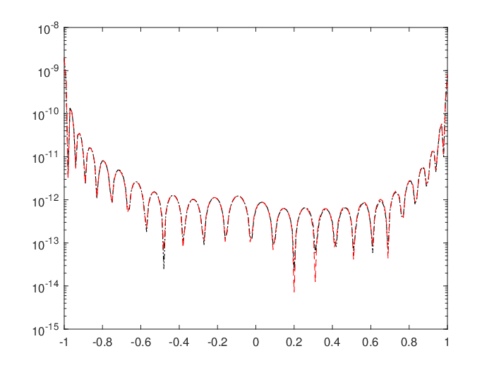
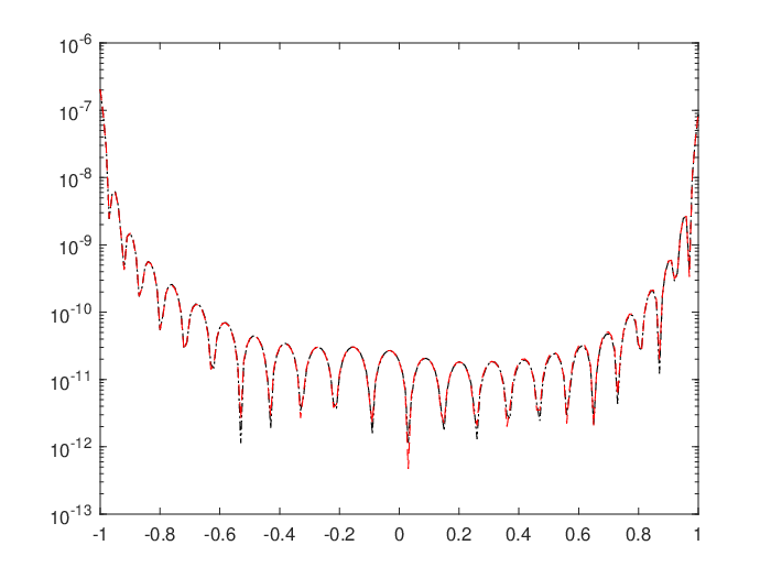
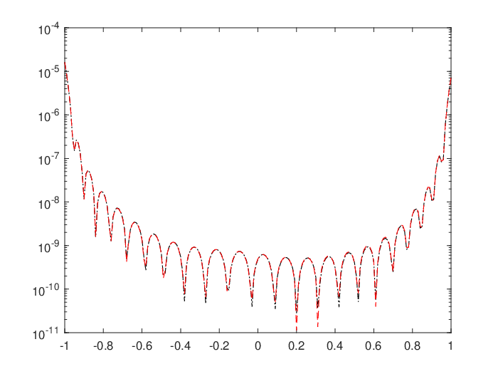
obtained in approximating the first four order derivatives of the function f1f_{1} by the constrained mock-Chebyshev least squares operator on the uniform grid of 6767 points in [−1,1][-1,1], computed by following the strategy S2S_{2}. In equation (35) eie_{i} is the absolute value of the approximation error at the ii-th point of this grid. The numerical results are reported in Table 2. The approximation accuracies are comparable or even better with respect to those one reported in [13] for the case of the finite difference formula at 1111 equally spaced points with stepsize h=0.03h=0.03 in the interval [0,0.3][0,0.3]. To better appreciate the behavior of the approximation errors in the whole interval [−1,1][-1,1], in Figure 6 we plot the absolute values of the pointwise errors computed on the equispaced grid of N=201N=201 points for the first four order derivatives of the function f1f_{1}. The plots are displayed in a lexicographic order, by increasing the order of derivatives. The red dash-dotted line is the error of approximation related to the application of the strategy S1S_{1} while the black dashed line is the error of approximation related to the application of the strategy S2S_{2}. From the Figure, it is evident that the application of the two strategies S1S_{1} and S2S_{2} gives practically the same results.

o​r​d​e​rorder 0 1 2 3 4
em​e​a​ne_{mean} 1.24e-15 7.59-14 9.02-12 9.92e-10 8.57e-08
em​a​xe_{max} 1.77e-14 4.43e-12 7.46e-10 7.67e-08 5.78e-06
Table 2: Mean and max approximation errors obtained in approximating the function f1​(x)=x​e−2​x+sin⁡(3​x)f_{1}(x)=xe^{-2x}+\sin(3x) and its first four order derivatives on the grid of 6767 equispaced points in [−1,1][-1,1], by using the constrained mock-Chebyshev least squares operator with n+1=67n+1=67.
Refer to caption
Refer to caption
Refer to caption
Refer to caption
Figure 6: Behavior of the approximation errors, in absolute value, of the first four order derivatives of the function f1​(x)=x​e−2​x+sin⁡(3​x)f_{1}(x)=xe^{-2x}+\sin(3x) in the whole interval [−1,1][-1,1], by using the constrained mock-Chebyshev least squares operator with n+1=67n+1=67. The absolute values of the pointwise errors are computed on the equispaced grid of N=201N=201 points. The plots are displayed in a lexicographic order, by increasing the order of derivatives. From the plots, it is evident that the application of the two strategies S1S_{1} (red dash-dotted line) and S2S_{2} (black dashed line) gives practically the same results.

In the second type of test, we consider the following functions [13, 12]

f1​(x)=x​e−2​x+sin⁡(3​x),f2​(x)=e−50​(x−0.4)2+sinh⁡(x),\displaystyle f_{1}(x)=xe^{-2x}+\sin(3x),\quad f_{2}(x)=e^{-50(x-0.4)^{2}}+\sinh(x),
f3​(x)=11+8​x2,f4​(x)=11+25​x2,\displaystyle f_{3}(x)=\frac{1}{1+8x^{2}},\quad f_{4}(x)=\frac{1}{1+25x^{2}},

and we analyze the trend of the mean approximation errors and the maximum approximation errors (35) obtained in approximating the first four order derivatives of f1−f4f_{1}-f_{4} by using the constrained mock-Chebyshev least squares operator on uniform grids of different stepsize. In particular, we consider sets of n+1n+1 equispaced nodes with n=50​kn=50k, k=1,…,80k=1,\dots,80 and compute the errors on a grid of N=105N=10^{5} random points of the interval [−1,1][-1,1].

The results of the tests are shown in Figures 7, 8, 9 10. All these examples show, with clear evidence, that once the maximum precision is reached for P^r,n​[f]\hat{P}_{r,n}[f], the increase in the number of nodes does not lead to more accurate approximation for the derivatives, on the contrary, the increase of the condition number of the matrices involved in the strategies S1S_{1} and S2S_{2} causes worsening of results.

Refer to caption
Refer to caption
Figure 7: Mean approximation error (left) and Maximum approximation error (right) at N=100000N=100000 random points in the interval [−1,1][-1,1] relative to the function f1​(x)=x​e−2​x+sin⁡(3​x)f_{1}(x)=xe^{-2x}+\sin(3x) (in blue) and its first four derivatives, with the increasing order from the bottom to the top, when approximated by using the constrained mock-Chebyshev least squares operator with n=50​kn=50k, k=1,…,80k=1,\dots,80. From the plots, it is evident that the application of the two strategies S1S_{1} (red) and S2S_{2} (black) gives practically the same results.
Refer to caption
Refer to caption
Figure 8: Mean approximation error (left) and Maximum approximation error (right) at N=100000N=100000 random points in the interval [−1,1][-1,1] relative to the function f2​(x)=e−50​(x−0.4)2+sinh⁡(x)f_{2}(x)=e^{-50(x-0.4)^{2}}+\sinh(x) (in blue) and its first four derivatives, with the increasing order from the bottom to the top, when approximated by using the constrained mock-Chebyshev least squares operator with n=50​kn=50k, k=1,…,80k=1,\dots,80. From the plots, it is evident that the application of the two strategies S1S_{1} (red) and S2S_{2} (black) gives practically the same results.
Refer to caption
Refer to caption
Figure 9: Mean approximation error (left) and Maximum approximation error (right) at N=100000N=100000 random points in the interval [−1,1][-1,1] relative to the function f3​(x)=11+8​x2f_{3}(x)=\frac{1}{1+8x^{2}} (in blue) and its first four derivatives, with the increasing order from the bottom to the top, when approximated by using the constrained mock-Chebyshev least squares operator with n=50​kn=50k, k=1,…,80k=1,\dots,80. From the plots, it is evident that the application of the two strategies S1S_{1} (red) and S2S_{2} (black) gives practically the same results.
Refer to caption
Refer to caption
Figure 10: Mean approximation error (left) and Maximum approximation error (right) at N=100000N=100000 random points in the interval [−1,1][-1,1] relative to the function f4​(x)=11+25​x2f_{4}(x)=\frac{1}{1+25x^{2}} (in blue) and its first four derivatives, with the increasing order from the bottom to the top, when approximated by using the constrained mock-Chebyshev least squares operator with n=50​kn=50k, k=1,…,80k=1,\dots,80. From the plots, it is evident that the application of the two strategies S1S_{1} (red) and S2S_{2} (black) gives practically the same results.

5 Conclusions

In this paper, we have analyzed the theoretical aspects of the constrained mock-Chebyshev least squares operator. We have introduced explicit representations of the error and its derivatives. By using the constrained mock-Chebyshev least squares operator, we have presented a method for approximating the successive derivatives of ff at any point x∈[−1,1]x\in[-1,1] and provided estimates for these approximations. This formula provides a global polynomial approximation of the successive derivatives of the function ff.

Acknowledgments

This research has been achieved as part of RITA “Research ITalian network on Approximation” and as part of the UMI group “Teoria dell’Approssimazione e Applicazioni”. The research was supported by GNCS-INdAM 2022 projects. The authors are members of the INdAM Research group GNCS.

References

  • [1] J. P. Boyd and F. Xu. Divergence (Runge phenomenon) for least-squares polynomial approximation on an equispaced grid and Mock–Chebyshev subset interpolation. Applied Mathematics and Computation, 210(1):158–168, 2009.
  • [2] S. Boyd and L. Vandenberghe. Introduction to applied linear algebra: vectors, matrices, and least squares. Cambridge University press, Cambridge, 2018.
  • [3] E. W. Cheney. Introduction to Approximation Theory. Courier Corporation, Massachusetts, 1998.
  • [4] P. J. Davis. Interpolation and Approximation. Courier Corporation, Massachusetts, 1975.
  • [5] S. De Marchi, F. Dell’Accio, and M. Mazza. On the constrained mock-Chebyshev least-squares. Journal of Computational and Applied Mathematics, 280:94–109, 2015.
  • [6] F. Dell’Accio, F. Di Tommaso, and F. Nudo. Constrained mock-Chebyshev least squares quadrature. Applied Mathematics Letters, 134:108328, 2022.
  • [7] F. Dell’Accio, F. Di Tommaso, and F. Nudo. Generalizations of the constrained mock-Chebyshev least squares in two variables: Tensor product vs total degree polynomial interpolation. Applied Mathematics Letters, 125:107732, 2022.
  • [8] N. Hale and A. Townsend. Fast and accurate computation of Gauss–Legendre and Gauss–Jacobi quadrature nodes and weights. SIAM Journal on Scientific Computing, 35(2):A652–A674, 2013.
  • [9] G. W. Howell. Derivative error bounds for Lagrange interpolation: an extension of Cauchy’s bound for the error of Lagrange interpolation. Journal of Approximation Theory, 67(2):164–173, 1991.
  • [10] B. A. Ibrahimoglu. A fast algorithm for computing the mock-Chebyshev nodes. Journal of Computational and Applied Mathematics, 373:112336, 2020.
  • [11] B. A. Ibrahimoglu. A new approach for constructing mock-Chebyshev grids. Mathematical Methods in the Applied Sciences, 44(18):14766–14775, 2021.
  • [12] G. Klein and J.-P. Berrut. Linear rational finite differences from derivatives of barycentric rational interpolants. SIAM Journal on Numerical Analysis, 50(2):643–656, 2012.
  • [13] J. Li. General explicit difference formulas for numerical differentiation. Journal of Computational and Applied Mathematics, 183(1):29–52, 2005.
  • [14] W. Markoff and J. Grossmann. Über Polynome, die in einem gegebenen Intervalle möglichst wenig von Null abweichen. Mathematische Annalen, 77(2):213–258, 1916.
  • [15] T. J. Rivlin. Optimally Stable Lagrangian Numerical Differentiation. SIAM Journal on Numerical Analysis, 12(5):712–725, 1975.
  • [16] T. J. Rivlin. Chebyshev Polynomials. Courier Dover Publications, New York, 2020.