Long-range data transmission in
a fault-tolerant quantum bus architecture
Abstract
We propose a scheme for fault-tolerant long-range entanglement generation at the ends of a rectangular array of qubits of length and a square cross section of size with . Up to an efficiently computable Pauli correction, the scheme generates a maximally entangled state of two qubits using a depth- circuit consisting of nearest-neighbor Clifford gates and local measurements only. Compared with existing fault-tolerance schemes for quantum communication, the protocol is distinguished by its low latency: starting from a product state, the entangled state is prepared in a time determined only by the local gate and measurement operation time . Furthermore, the requirements on local repeater stations are minimal: Each repeater uses only qubits with a lifetime of order . We prove a converse bound on the number of qubits per repeater among all low-latency schemes for fault-tolerant quantum communication over distance . Furthermore, all operations within a repeater are local when the qubits are arranged in a square lattice.
The noise-resilience of our scheme relies on the fault-tolerance properties of the underlying cluster state. We give a full error analysis, establishing a fault-tolerance threshold against general (circuit-level) local stochastic noise affecting preparation, entangling operations and measurements. This includes, in particular, errors correlated in time and space. Our conservative analytical estimates are surprisingly optimistic, suggesting that the scheme is suited for long-range entanglement generation both in and between near-term quantum computing devices.
1 Introduction
The ability of operating on spatially separated qubits has been recognized early on as a key requirement for a working quantum computer [12, 47]. Long-range quantum communication is also a fundamental primitive at the core of quantum information-theoretic [22, 28, 54] and cryptographic [3, 21] protocols in quantum networks, as well as e.g., distributed quantum computation [7, 36, 49] or distributed sensing [29, 16]. With increasingly powerful capabilities of present-day devices that can act as local nodes in such a network, finding appropriate protocols for entanglement sharing and quantum communication over faulty networks remains an active and central theme of present-day research.
The nature of the best protocol to be used depends heavily on the available hardware and its noise characteristics. Here we consider a monolithic architecture for point-to-point communication in a quasi-1D array of qubits. In terms of more standard terminology in quantum communication, this scheme can be interpreted as consisting of a line of repeater stations. Our proposal addresses the specific constraints on near-term devices by optimizing the following aspects:
- (i)
minimal number of qubits per repeater station: As a function of the total communication distance , every repeater only needs to manipulate number of qubits. This is in line with the best currently known proposals for long-range quantum communication. We also provide a converse bound on the number of qubits per repeater for low-latency protocols as considered in this work.
- (ii)
short coherence times: The required coherence time of each qubit is independent of the overall communication distance : It only needs to be of the order of the local operation time . This is the maximal time needed to perform a single- or two-qubit gate, a single-qubit measurement, or an entangling gate between two neighboring repeaters.
- (iii)
simplicity of involved operations: Our scheme only involves one- and two-qubit gates between nearest-neighbor qubits in the architecture. In particular, assuming the repeater stations are connected appropriately, all operations at each repeater are geometrically local when the qubits are arranged on a 2D array. This makes the scheme particularly attractive for, e.g., planar chip-like devices where the connectivity to neighboring devices is established through the third dimension.
Because of the simplicity of the scheme, we can explicitly specify and analyze all involved operations without resorting to fault-tolerant gadgets (e.g., for encoding and recovery) that are often treated in a black-box manner. In particular, this means that we can provide a stringent error analysis for fully general circuit-level noise.
- (iv)
resilience to general errors: we provide a rigorous proof of the robustness of our scheme in the form of a fault-tolerance threshold theorem allowing for general local stochastic noise. This models not only the commonly studied situation where qubits are depolarized according to identically and independently distributed errors (i.e., product channels), but also captures situations where errors are correlated both in space and time. We assume all involved operations (state preparation, gates and measurements) to be non-ideal, i.e., affected by noise.
- (v)
minimal latency: Our protocol minimizes the “time to entanglement” , the amount of time it takes to establish long-range entanglement from a product state of all qubits. The long-range entangled state is available after a time of order . In contrast, the quantity scales at least linearly with the total communication distance in several existing protocols based, e.g., on transmitting encoded information successively between neighboring repeaters.
We note that some of these protocols reach the scaling per generated Bell pair asymptotically when operated continuously, i.e., this is an achievable rate of communication. In contrast, the quantity measures the latency when starting to run the scheme, and may be particularly relevant in near-term applications in scenarios where continuous operation is challenging.
We note that our analysis treats Pauli errors and erasure errors on the same footing (similar to e.g., Refs. [42]) leading to a fault-tolerance threshold for situations where the noise strength of both of these types of noise is of the same order of magitude. Future work may examine using modified decoders [9] exploiting the high loss tolerance of topological codes [2]; indeed, we expect these schemes to be resilient to loss errors with a probability of occurrence closer to the percolation threshold of the square lattice, i.e., much higher than the thresholds we establish for local stochastic Pauli noise.
Because of the simplicity of the involved operations, our scheme is a candidate architecture for transferring quantum information between as well as within quantum devices. That is, it can act as a data bus which can exchange information between various components as first studied in [5]. Because it prepares a Bell pair up to an (efficiently computable) Pauli error, it is compatible with e.g., magic-state injection methods to achieve universality: corrections can be propagated “in software”, i.e., by commuting Pauli operators through a stabilizer circuit without the need for physically applying a correction before proceeding with the computation.
In the area of quantum computing architectures, our protocol could be especially beneficial in settings where gates or measurements need to performed between spatially distant qubits. Such a need arises for example when using a quantum low-density parity check (LDPC) code whose stabilizer generators are not spatially local. With our scheme, we can design a quasi-2D architecture that allows for the application of joint measurements on any subset of size of a total of qubits, see Fig. 1. Each such -qubit measurement is executed with constant fidelity in a constant amount of time (up to Pauli correction whose classical postprocessing can typically be deferred to a later stage). The architecture requires qubits in total. When combined with the recently discovered good quantum LDPC codes that have parameters close to optimal [44], this logarithmic overhead unfortunately only leads to an encoding rate that decays as an inverse polylogarithmic function. In the near term, however, this still beats e.g., surface-code based approaches [8, 32] that have an inverse polynomial encoding rate, although the latter have the advantage of being strictly 2D and not quasi-2D as our scheme.

Prior work on entanglement generation from cluster states
Our work builds on the fault-tolerance properties of the 3D cluster state. In seminal work [48], Raussendorf, Bravyi and Harrington proved that for temperatures below some threshold, the thermal state of the cluster state Hamiltonian on a simple 3D cubic lattice has localizable entanglement: applying single-qubit Pauli measurements to each “bulk” qubit results – up to Pauli corrections determined by the measurement outcomes – in an encoded Bell state of 2D surface codes lying on two opposing faces of the cube. Since the initial thermal state is the cluster state with independent and identically distributed Pauli--errors on each qubit, and the cluster state can be created in constant depth with local operations, this provides a scheme for long-range (encoded) entanglement generation by a constant-depth circuit with local gates. While the assumed (physically motivated) noise model is somewhat restricted, the authors of [48] also point out that more general errors on the initial cluster state such as independent single-qubit depolarizing noise can be tolerated when using ideal (non-faulty) operations at the two surfaces.
Entanglement generation in a cubic lattice can indeed be achieved under more general noise: As shown in [4], the Raussendorf-Bravyi-Harrington scheme produces a logical Bell pair even under general local stochastic noise below some threshold. Local stochastic errors model general circuit-level Pauli noise that can include correlations in time and space. As a special case, this encompasses independent and identically distributed (i.i.d.) Pauli noise on the initial cluster state, as well as e.g., measurement errors. We discuss this error model and the exact statement of [4] below. It shows that under local stochastic noise, it is possible to generate an encoded Bell pair which is corrupted by a residual local stochastic error. The latter can be corrected by surface-code decoding.
The scheme of [48] produces a surface-code encoded Bell pair, i.e., the resulting entanglement lives in a logical -qubit subspace of a many-qubit system. In applications such as the one considered in [4], this is a desirable feature: the encoded information can be operated on without decoding, thus preserving fault-tolerance properties. In a communication scenario, however, it may be more desirable to establish entanglement between two physical qubits instead. A scheme for achieving this kind of localization of the entanglement was proposed in [45] by modifying the approach of [48]: Here a different single-qubit measurement pattern is used at the two (“surface code”) boundaries. This results in entanglement between two distinguished qubits in each surface. For the problem of establishing a constant-fidelity Bell pair in a cube of size , the work [45] provides analytical and numerical threshold estimates in the case of i.i.d. Pauli- and Pauli- errors in the cluster state. (It was argued in [45] that this error model captures a situation where initially, independent noisy Bell states are shared along each edge of the cubic lattice, and all subsequent (single-qubit) operations are ideal, i.e., noise-free.) In particular, it is shown that there is a threshold error rate such that constant-fidelity two-qubit entanglement (i.e., independent of ) is established for any error rate below that threshold.
To achieve long-distance communication, one can use cluster states on lattices of the form with , i.e., lattices that are elongated in the direction where quantum information is to be transferred. In this work, we denote a lattice of such form by , see Section 6 for a detailed definition. The corresponding setup is quasi-1D, with qubits arranged on a square on each “slice” along this direction. This idea has been explored numerically in the case of i.i.d. Pauli- noise in [48]. For sufficiently small error rates, a fidelity of the encoded (error corrected) scaling as for some constants was observed. These simulations were carried out for period boundary conditions. Assuming the surface codes have similar behavior as toric codes away from the threshold, this implies that using (i.e., a polylogarithmic number of qubits per repeater station) is sufficient to achieve constant fidelity over a distance . In a similar vein, the results of [45] are stated for cubes (i.e., lattices of the form ), but the author suggests using lattices of the form with . Here we establish rigorous bounds on the fault-tolerance threshold for this scenario for a more general noise model.
Surface codes for communication and as topological quantum memories
Our work is closely related to [45]: indeed, the cluster state and measurement pattern used in our scheme is identical to that of [45]. As we explain below, this measurement strategy and the associated correction operation can be interpreted as a fault-tolerant single-shot decoding procedure for the surface code. In fact, the corresponding measurement pattern for the surface code has also previously been used in [33] to realize a fault-tolerant -measurement. A similar triangular pattern has been applied in Refs. [35, 34] for encoding, i.e., state preparation, for the surface code, and more specifically, for injecting a magic state into the surface code [31].
Surface codes have found many uses in information-processing and communication settings. While some of these proposals are superficially similar to our work, they typically have different objectives. In particular, they often involve operations over an extensive amount of time, preventing realization by a constant-depth circuit: Consider first the fault-tolerant encoding/decoding scheme for the 2D surface code studied in [34]. This scheme establishes entanglement in time, i.e., gives a complete prescription (including preparation and readout) of how the surface code can be used to preserve quantum information. Similar to the seminal work [10] showing that the surface code can be used as a quantum memory even with noisy syndrome measurements, this leads to a matching problem on a 3D lattice in spacetime. This is conceptually different from our procedure: Our decoding procedure involves a “spacelike” 3D lattice, and the entire process is achieved in a constant time. (Ref. [34] also gives a lower bound on the achievable fidelity in terms of “circuit volume” when using concatenated codes. The non-locality and complexity of the involved operations is mentioned as a challenge.)
The proposal of [19] also relies on surface codes: Several corresponding code patches are placed next to each other along the communication direction and an encoded qubit is teleported through this architecture. Similar to a topological quantum memory with noisy syndrome measurements, the scheme relies on interaction and measurement patterns that are repeated a number of times scaling linearly with the code distance.
Local stochastic noise and Clifford circuits
We consider quantum circuits subject to local stochastic noise. This is a general notion of errors introduced in [23] to model situations where the noise is “locally decaying” but otherwise arbitrary. In particular, this model includes not only i.i.d. noise on each qubit, but also adversarial settings where errors can have unspecified correlations both in space and time (i.e., at different circuit locations).
Here we follow the formalism used in [17]. When implementing an ideal circuit under local stochastic noise, all qubits experience a random Pauli error at each time step (gate layer) of the circuit. The only assumption we make is that high-weight errors are exponentially suppressed as quantified by a parameter called the noise strength. To be specific, consider a quantum circuit using qubits. A Pauli error is a random variables on the -qubit Pauli group. Its support is the (random) subset of qubits it acts on non-trivially, i.e., with either , , or . We call a Pauli error a local stochastic error with strength , written , if any subset of qubits is affected by with probability at most , i.e., if
| (1) |
Consider an ideal depth- circuit that starts in a product state of qubits, applies a unitary
| (2) |
consisting of gate layers (each of which is a depth- circuit consisting of one- and two-qubit gates) and subsequently measures a subset of the qubits in the computational basis. We call a noisy execution of this circuit with parameter the same kind of process, but with replaced by
| (3) |
where each error
| (4) |
is a local stochastic error with strength . This models both preparation errors (described by ), gate execution errors (described by for ) and measurement errors, i.e., bit flips in the measurement outcome (described by ). Importantly, the random variables need not be independent, capturing situations where errors are correlated in time. Indeed, condition (4) merely imposes constraints on the marginal distributions of the errors .
Put succintly, the goal of fault-tolerance is to design an ideal circuit in such a way that any noisy implementation of the circuit still realizes the desired functionality, assuming that the error strength is below some threshold. The noise model considered here makes the corresponding analysis tractable when working with Clifford circuits: Any local stochastic error can be commuted forward or backward (in time) through such a circuit while preserving the property of being a local stochastic error. In addition, products of local stochastic errors are themselves local stochastic errors, meaning that errors can be accumulated, i.e., combined into a single local stochastic error. These manipulations change the error strength. More precisely, it is possible to establish conservative upper bounds on the error strength of the resulting error, see [4, Lemma 11] for a formal statement of this calculus of local stochastic errors. Importantly, however, these manipulations do not change the nature of the errors: This is because of the minimal assumptions used in the definition of local stochastic noise.
We note that the practice of commuting Pauli errors forward or backward through a circuit composed of Clifford gates is common throughout the literature. However, in some earlier work on quantum repeaters, the fact that such operations may introduce correlations between errors when starting from an i.i.d. error model is sometimes neglected. The concept of local stochastic errors and the corresponding calculus elegantly sidesteps this difficulty: For any Clifford circuit of constant depth , it is sufficient to establish resilience against a single local stochastic error at any time step in the circuit, rather than considering the -tuple : Indeed, any noisy circuit (3) behaves identically to a circuit of the form
| (5) |
with a certain local stochastic error . A corresponding upper bound on the error strength follows by applying commutation relations and combining errors according to rules such as those given in [4, Lemma 11].
Single-shot encoded Bell state preparation and surface code readout
To exemplify this line of reasoning, consider the (ideal) circuit studied [4]. Starting from a product state , it applies a depth- circuit with nearest-neighbor Clifford gates to prepare the cluster state on a lattice . Subsequently, a subset of qubits is measured in the computational basis, yielding an outcome (string ). Up to a Pauli correction determined by the measurement outcome , this circuit prepares logical Bell state encoded in two surface codes on the two boundaries of the lattice, that is, we have
| (6) |
Now consider a noisy execution of this circuit. There are three sources of error: Errors in the preparation of the initial state , errors during the execution of the circuit , and errors affecting the single-qubit measurements. The former two types of errors can be commuted forward in time past the last gate layer of . Measurement errors (where an error on a single qubit measurement corresponds to a Pauli--error before application of the ideal measurement) can be commuted backwards in time. Combining the commuted versions of these errors, it thus suffices to consider the case where a single local stochastic error is applied after the execution of . All other operations may be assumed to be ideal, i.e., noise-free: The overall process is equivalent to measuring (using an error-free measurement) a noisy cluster state , corrupted by a local stochastic error .
What does a noisy execution of the circuit achieve? It turns out that the procedure still prepares the logical Bell state up to the known Pauli correction (depending on the measurement result ) and an additional residual error (depending on the local stochastic error ). The main technical result established in [4] for this “single-shot preparation procedure” shows that this residual error itself is local stochastic, and its error strength can be related to the error strength of the original local stochastic error . Let us state the corresponding result since it motivates our construction.
Theorem 1.1 (Single-shot encoded Bell state preparation [4]).
Suppose . Then there is a threshold probability such that the following holds: Let be the cubic lattice of linear size with one qubit per site. Let be a local stochastic error with error strength . Then there is a local stochastic error with
| (7) |
such that
| (8) |
with certainty, where the probability is taken over the choice of and the syndrome (measurement result) .
We note that Theorem 1.1 primarily constitutes a proof-of-principle, giving a precise formulation of the idea that the final state is the encoded Bell state up to a locally decaying error. Both the threshold error strength obtained, as well as the exponent in (7) are likely to be more conservative bounds than necessary in reality, and are expected to be too demanding for experimentally relevant parameters ranges. Nevertheless, Theorem 1.1 shows that the single-shot encoded Bell state preparation procedure can be combined with suitable surface code protocols that are resilient to local stochastic errors. Indeed, this is the way the cluster state is used in the application of [4] and follow-up work [25, 37].
One such noise-resilient surface code protocol is the single-shot decoding protocol discussed in [4]. It shows that measurement of the logical Pauli- operator in the surface code can be achieved fault-tolerantly by local operations even in the presence of local stochastic noise. Let us paraphrase the corresponding statement here.
Theorem 1.2 (Single-shot logical -measurement [4]).
Consider a surface code of distance with qubits. Let be a local stochastic error with strength . Then there is a function such that the following holds. Let be an arbitrary encoded state. Assume we measure every qubit of the state in the computational basis obtaining the outcome . Then
| (9) |
where
| (10) |
(We note that without loss of generality, the error can be assumed to be consisting of Pauli- operators only.)
Since is the probability of observing the outcome when measuring the logical -operator, Theorem 1.2 provides a way of fault-tolerantly performing a measurement of this operator. While we do not directly use this result, it is part of the motivation for our single-shot decoding procedure and its analysis.
Prior work on quantum repeaters
A comparative study of different approaches to long distance quantum communication is provided in [42] where the authors discuss three generations of quantum repeater protocols:
The first generation of quantum repeaters is based on heralded entanglement generation between neighboring stations or repeaters (where entanglement is generated using post-selection on suitable measurement outcomes) combined with heralded entanglement purification (where multiple imperfect Bell pairs are used to probabilistically produce higher-fidelity Bell pairs) [6, 51]. These steps are repeated recursively at different distance scales. First-generation protocols of this kind require at a number of qubits polynomial in the total communication distance at each repeater station. The rate (i.e., number of Bell pairs established per channel use) is an inverse polynomial in , and the total time per Bell pair is given determined by , where is the gate time and the speed of light (corresponding to classical data transfer).
Second-generation protocols make use of heralded entanglement generation to counteract loss errors, and use quantum error-correcting codes to deal with operation errors: long-range encoded entanglement is generated by (encoded) entanglement swapping [27, 39, 55]. This leads to a reduction in classical two-way communication previously required in the entanglement purification step. The communication rate is improved to an inverse polylogarithmic function of , whereas the overall time-scale still scales as .
Protocols of the third generation use quantum error correcting codes to address not only operation errors, but also qubit loss [19, 41, 43, 40]. This family of protocols proceeds by communicating encoded quantum information: Repeaters apply a recovery operation to each codeblock before retransmitting the entire block to the next repeater. Because this family of protocols can be realized using one-way communication only, it requires little time per transmitted qubit: The time taken per transmitted qubit is only limited by , where is the local gate operation time. This advantage comes at the cost of requiring relatively high-fidelity quantum gates to realize the error correction operation at each repeater. The achieved rate in this generation of protocols is an inverse polylogarithmic function of .
Our work is a close relative to these third-generation protocols: indeed, one interpretation of the corresponding architecture is that it encodes logical information into a surface code at each repeater station. We emphasize, however, that this only motivates the scheme similar to the way e.g., cluster-state measurement-based quantum computation is related to braiding surface code anyons. For example, the scheme does not involve intermediate encoding/recovery operations associated with these surface codes.
Purely error-correction based schemes such as those of the third generation have a loss-tolerance limited by 50% because of the no-cloning theorem. To sidestep this limitation, the more recent work [56] combines error correction with hashing-based entanglement purification. In this scheme, intermediate error correction operations are realized based on stabilizer (resource) states prepared at each repeater. The proposed scheme achieves a constant rate of qubit transmission. Here error correction is based on measurement-based gate teleportation using special (graph) states encoding the recovery map at each repeater location. While such schemes are ultimately desirable, the generation of these resource states is arguably more challenging to realize with near-term devices than the protocol discussed here.
2 Our contribution: Main ideas and results
A threshold theorem for long-range entanglement generation
In this work, we present a protocol for generating a long-range entangled two-qubit Bell state in a fault-tolerant manner in the presence of local stochastic noise. It is based on a 3D cluster state on a lattice of the form , see Fig. 2.

To state our main result, we use the following notations: We let denote the set of qubits on the cluster state lattice . For a subset , we write for the all-zero basis state on the qubits . Similarly, we write for the product of single-qubit Hadamard operators on each qubit of . When measuring a subset in the computational basis, we denote the measurement result by , where consists of one measurement outcome bit associated with each qubit . The standard two-qubit Bell state is denoted
| (11) |
and the two-qubit Bell basis consists of the Bell states
| (12) |
Our main result is the following fault-tolerance threshold theorem:
Theorem 2.1 (Long-range entanglement generation).
Let with and be odd with . Assume that
| (13) |
There is a partition
| (14) |
of the set of qubits into disjoint sets , and a set consisting of two qubits located at opposite ends of , with coordinates and , respectively, as well as two efficiently computable functions
| (15) |
such that the following holds. Consider the following protocol:
- (i)
Prepare the cluster state by applying the local depth- Clifford circuit to qubits associated with the cluster state lattice .
- (ii)
Measure each qubit except the two distinguished qubits according to the following pattern:
- (a)
Each qubit is measured in the Hadamard basis
- (b)
Each qubit is measured in the computational basis.
Let be the (collection) of measurement outcomes.
- (a)
Assume that the state after step (i) is corrupted by a local stochastic error of strength
| (16) |
Let
| (17) |
be the post-measurement state on qubits . Then the post-measurement state on qubits is the Bell basis state with probability at least
| (18) |
Recall that the cluster state lattice has qubits in each “sheet” (with fixed coordinate ) along the communication direction. This is the number of qubits that our protocol uses at each repeater station. Eq. (13) thus implies that, to produce constant-fidelity two-qubit entanglement (under constant-strength noise), our protocol uses or
| (19) |
That is, the number of qubits per repeater station is polylogarithmic in the communication distance for our protocol. We give a converse bound, see Theorem 2.2 below.
The functions and involve solving minimum matching problems on certain sublattices of . With Edmond’s algorithm [14, 30, 20, 53], they can be evaluated in a time . In the context of surface code decoding, it has been shown that parallel processing leads to a polylogarithmic runtime instead [13, 11]. We expect that similar approaches are applicable here.
Our scheme is essentially identical to the procedure of [45], but constructed in a modular manner: We introduce a new primitive we call single-shot decoding of surface codes. Combining this with the Raussendorf, Bravyi and Harrington-scheme [48], i.e., applying single-shot decoding to each of the two surface codes yields our scheme. Our work thus gives a reinterpretation of the scheme [45] along with a more general error analysis.
Optimality: A converse to the threshold theorem
We study to which extent the protocol provided by Theorem 2.1 is optimal among protocols with low latency, i.e., where the entanglement is created after a constant amount of time (modulo local correction operations). Specifically, we consider protocols that are given by constant-depth quantum circuits, and ask if the relationship between the number of qubits at each repeater station and the communication distance can be better than polylogarithmic (cf. (19)). We find that this is not the case, i.e., the scaling of our protocol is essentially optimal.
The class of protocols we consider are given by constant-depth circuits. A depth- circuit for entanglement generation
- (i)
starts with a product state among all qubits, where each repeater (site) has qubits,
- (ii)
applies a depth- circuit consisting of single-qubit measurements, single-qubit gates and two-qubit gates between qubits at a repeater (site) and/or between nearest-neighbor sites. Constant-depth here means that is a constant (independent of ).
- (iii)
returns a state on two qubits located at the two ends of the communication line at distance . This state is supposed to be the Bell state up to a local (i.e., tensor product) correction that can be computed from the measurement outcomes.
We allow for adaptivity, i.e., unitaries can be classically controlled by measurement outcomes obtained during the execution of the circuit. Our main no-go result applies to all such protocols irrespective of whether or not the classical computations determining these adaptive actions are efficient.
Our protocol is of this kind (for qubits arranged on the cluster lattice ). Also of this kind are protocols proposed in the seminal work [1] on “entanglement percolation”. The work [1] considers a unitary error model where the resource state has a non-maximally entangled Bell state on each link. In addition to proposing protocols for this setting for 2D networks, it is shown in [1] that for a 1D chain of qubits, long-distance entanglement cannot be created by any single-shot protocol: Assuming any constant error per link, the fidelity of the resulting Bell state decays exponentially with distance.
We prove a converse to our “achievability” Theorem 2.1. It generalizes the statement of [1] to a setting where instead of a single (pair) of qubits per site (along the communication line), each site can have a polylogarithmic number of qubits. In addition, we allow constant-depth circuits instead of local measurements only. We find a local stochastic error of constant strength which leads any such protocol to fail if the communication distance is too large compared to the number of bits at each repeater station. That is, we show the following, see Corollary 8.1 for a detailed version of this bound.
Theorem 2.2 (Converse for low latency schemes).
Let be a protocol for long-range entanglement generation over distance which
- (i)
uses qubits per repeater,
- (ii)
is realized by a constant-depth (adaptive) circuit
- (iii)
is resilient to arbitrary local-stochastic noise of strength below a constant threshold , i.e., produces a constant-fidelity Bell pair.
Then we must have
| (20) |
The proof of Theorem 2.2 replaces the analysis of a low-latency protocol by that of an entanglement-assisted protocol , and follows from the fact that for any , the qubit depolarizing channel is a convex combination of an entanglement-breaking channel [26] and the identity channel (see Section 8.1 for details). It implies that local stochastic noise with any constant noise strength prevents entanglement generation over distances greater than exponential in the number of qubits at each site. In particular, it shows that the protocol discussed in Theorem 2.1 is essentially optimal among all low-latency protocols: Comparing (20) with (19), we conclude that the polylogarithmic scaling of the number of qubits per site in the protocol of Theorem 2.1 can at best be improved to a logarithmic scaling in .
Closing the log-factor gap between the converse Theorem 2.2 and achievability Theorem 2.1 appears to require a new approach, however: We can show that the analysis of Theorem 2.1 leading to the scaling (19) is tight. In fact, the scaling is necessary for any procedure which is based on the cluster state and uses the same syndrome information using functions and as in our protocol: We show the lower bound
| (21) |
for any such protocol (see Theorem 8.4 for a detailed statement). This result is obtained by a detailed analysis of the associated decoding problem, see Section 8.2. It applies, in particular, to natural variants of our scheme that are obtained, e.g., by replacing Edmond’s minimal matching algorithm by other procedures, including heuristic algorithms. This indicates that improving over our protocol will require a different resource state or measurement pattern.
Combining cluster-state generation and single-shot decoding
Let us briefly discuss the main ideas underlying our work, giving a high-level overview focused on the two main building blocks:
- (a)
The generation of a cluster state on an elongated lattice and subsequent single-qubit measurement of “bulk” qubits located at sites not belonging to the two boundaries with third coordinate equal to and , respectively. Up to local unitaries, this part of the procedure is identical to the original scheme of [48]. As shown in [4] (see Theorem 1.1 above), this generates a surface-code encoded Bell pair up to a (computable) Pauli correction and residual local stochastic noise.
- (b)
A novel single-shot decoding procedure for transferring surface-code encoded quantum information onto a single physical qubit. We show that this procedure is resilient to local stochastic noise: There is a threshold such that if the initial encoded state is corrupted by a local stochastic with noise strength , then the fidelity of the resulting single-qubit state with the logical state is exponentially close to as a function of the code distance . We refer to Theorem 2.3 below for details.
From a conceptual point of view, it is clear that combining (a) with (b) results in a procedure for generating long-range entanglement: Theorem 1.1 guarantees that the state after the first part of the procedure is essentially an encoded Bell state corrupted by a local stochastic error. Applying the single-shot decoding procedure to each of the two surface codes then results in a high-fidelity two-qubit Bell state. Indeed, our result (Theorem 2.3 below) ensures that the local stochastic error is dealt with properly in the single-shot decoding phase.
While our scheme for long-range entanglement generation is indeed a direct combination of steps (a) with (b), our analysis of the resulting fidelity is not simply a combination of the analytical results stated above for each module (a) and (b). This is because a naive combination of these analytical building blocks only provides a proof-of-principle: A threshold result derived in this way does not yield parameters of practical relevance. Instead, we establish a significantly tighter threshold estimate by a direct analysis of the achieved fidelity for the entire (combined) process.
Fault-tolerant single-shot decoding for surface codes
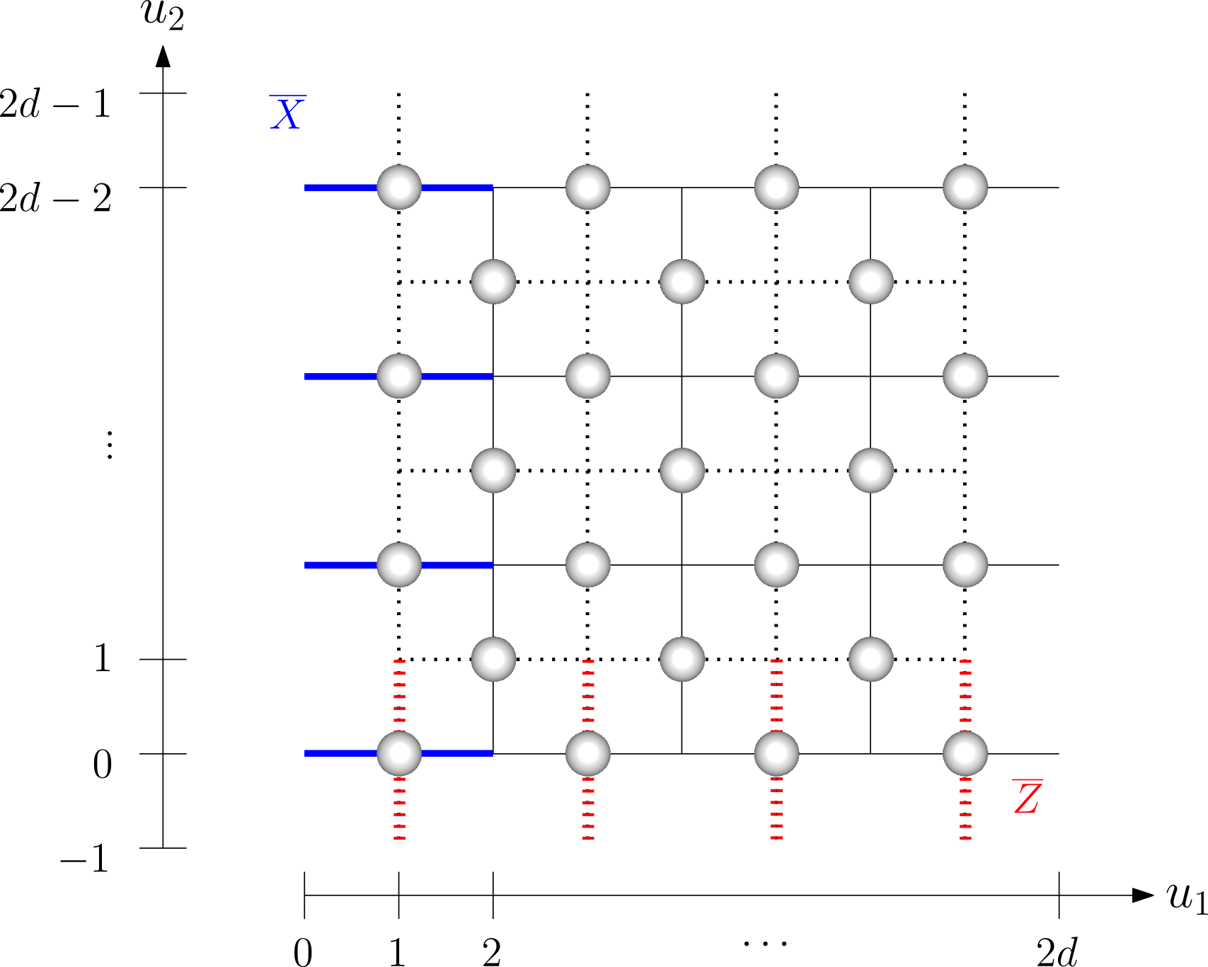
In the following, we consider a single qubit encoded into a surface code using an isometric encoding map that maps the single-qubit Pauli operators to the “canonical” logical string operators and of the surface code, see Fig. 3. Let us write for the encoded version of a physical qubit . Our main building block is a decoding procedure for the surface code that can be summarized as follows. It is illustrated in Fig. 4.

Theorem 2.3 (Single-shot surface code decoding).
Consider a distance- surface code with consisting of qubits. Then there is a partition of the set of qubits into disjoint sets , and a set consisting of a single qubit , and two efficiently computable functions
| (22) |
such that the following holds. Consider the following protocol applied to a surface-code encoded logical state corrupted by a local stochastic error of strengh
| (23) |
where is arbitrary:
- (a)
Each qubit is measured in the Hadamard basis, and
- (b)
each qubit is measured in the computational basis.
Let be the (collection of) measurement outcomes, and let
| (24) |
be the corresponding post-measurement state on qubit . Then
| (25) |
This shows that the logical state encoded in the surface code can be transferred to a single qubit in a fault-tolerant manner, up to a Pauli correction which is determined by the measurement outcomes. We refer to Theorem 5.7 below for a more detailed statement. Similarly as before, the functions are defined in terms of minimum matchings, and can be computed in time in this case.
We note that Theorem 2.3 immediately yields a protocol for fault-tolerantly measuring the logical Pauli- operator, thus subsuming Theorem 1.2. The corresponding measurement protocol proceeds by applying a computational basis measurement on the post-measurement state on qubit with outcome , and outputting the corrected bit . In a similar manner, one can realize a fault-tolerant logical -measurement as considered in [33]. Beyond measuring or , Theorem 2.3 also permits to execute any logical measurement on the encoded information. More generally, as the information ends up being localized on qubit , it can be acted on in subsequent quantum-information-processing protocols.
The protocol provided in Theorem 2.3 bears some similarity to teleportation: encoded information is essentially teleported to a single physical qubit. To illustrate the basic underlying idea, consider a CSS-stabilizer code encoding a single qubit, with a property that logical - and -Pauli operators can be chosen in a way that they overlap only in a single qubit . As a concrete example, consider the stabilizer code with generators
| (26) | ||||
| (27) |
It encodes a single logical qubit into three physical qubits. We can choose logical operators as
| (28) | ||||
| (29) |
which has the desired property (with being the first qubit). Suppose is an encoded state associated with . Assume we measure qubit in the Hadamard basis, obtaining outcome , and measure qubit in the computational basis getting the outcome . This corresponds to measuring the observables and . Then it is easy to check that the post-measurement state on qubit has expectation values
| (30) | ||||
| (31) |
It follows immediately that the state has identical expectation values as the logical state , and hence must be proportional to . That is, the logical state is decoded, i.e., transferred to the first physical qubit. We note, however, that the process described here is not fault-tolerant. In particular, the measurement of the observables and is not resilient to errors and may lead to an incorrect “correction” operation .
Here we argue that for the surface code, an analogous process can in fact be made fault-tolerant. The idea is to use logical operators that again only overlap in a single qubit , i.e.,
| (32) | ||||
| (33) |
where and are disjoint subsets of qubits, see Fig. 4. The goal, then, is to fault-tolerantly measure the observables and . Such a procedure can be obtained by modifying the protocol of Theorem 1.2. The latter gives a fault-tolerant way of measuring by measuring all qubits in the computational basis, and, by considering the dual lattice, a way of measuring the logical operator by measuring all qubits in the Hadamard basis. To simulate the measurement of both and at the same time, we use a pattern of single-qubit measurements that simultaneously measures a subset of qubits in the computational basis, and a subset of qubits in the Hadamard basis. The measurement pattern is “triangular” as shown in Fig. 4. We show that this procedure has the properties stated in Theorem 2.3.
Outline
In Section 3, we introduce our single-shot decoding protocol for the surface code accompanied with background material. In Section 4, we provide a combinatorial framework for analyzing matching problems arising in the analysis of both our surface code decoding protocol and the entanglement generation protocol introduced in Section 6. Using the framework, we prove in Section 5 that our surface code decoding protocol is robust against local stochastic noise.
Then in Section 6, we introduce our long-range entanglement generation protocol. We prove in Section 7 that this protocol is resilient against local stochastic noise of strength below a certain threshold: A lower bound on the achievable distance of entanglement generation is presented in terms of the noise strength and the number of qubits. Finally, in Section 8, we present a converse result for low latency entanglement generation schemes.
3 Single-shot surface code decoding
In this section, we define our single-shot decoding protocol for the surface code: We introduce all relevant definitions to apply this protocol in practice. We defer the analysis of the resilience of this protocol against local stochastic noise to subsequent sections: In Section 4, we will first provide general bounds on certain matching problems on graphs. These will subsequently be applied in Section 5 to establish a fault-tolerance threshold theorem for the single-shot decoding protocol introduced here.
3.1 Definition of surface code
We consider a distance--surface code with a total of qubits associated with horizontal edges and vertical edges as illustrated in Fig. 5. The code has smooth boundaries at the top and bottom, and rough boundaries on the left and right. In more detail, consider a square lattice in consisting of sites
| (34) |
We place qubits at sites with the property that one coordinate is even, whereas the other coordinate is odd, i.e., qubits are located at the sites
| (35) |
Here and below we write (respectively ) for an even (respectively odd) integer and use the convention that e.g., is the subset of all pairs with both and even. Let
| (36) |
denote Manhattan distance between and . Given a site , the set of nearest neighbors of is defined as
| (37) |
i.e., the nearest neighbors of are associated with qubits at Manhattan distance from .
The surface code graph is defined as
| (38) | ||||
| (39) |
In other words, edges of are associated with pairs separated by a distance , with the exception of pairs that lie on the same vertical at or . The corresponding vertices
| (40) |
are degree- vertices in , i.e., endpoints of “dangling” edges at one of the “rough” boundaries of : they are connected only to their right respectively left nearest neighbor. We can therefore express the set of edges of succintly as
| (41) |
In the following, it will be convenient to label an edge by its midpoint .
We will extensively use a “dual graph” . To define this, let us first consider the set
| (42) |
of dual sites. We note that the location of qubits can equivalently be specified as
| (43) |
i.e., . The dual surface code graph is defined by
| (44) | ||||
| (45) |
Here degree--vertices, i.e., those belonging to
| (46) |
are located at the top- and bottom “rough” boundaries. Again, we sometimes refer to an edge by its midpoint .
The surface code associated with the surface code graphs is defined as follow: For every vertex with degree , i.e., every vertex which is not the endpoint of a dangling edge , there is a stabilizer generator consisting of Pauli- operators only. Pauli--stabilizer generators are defined similarly based on the dual graph : For every , there is a stabilizer generator consisting of Pauli- operators only.


3.2 Graphs with internal vertices: boundary map and minimal matchings
Our decoder is based on an algorithm which finds certain matchings of a graph with internal and external vertices. Let us first discuss some basic notions.
We consider pairs where is a graph and a subset of vertices we call internal vertices. The complement will be referred to as the set of external vertices.
Define a boundary map that takes a subset of edges to a subset of internal vertices: An interval vertex belongs to if and only if the number of edges incident on is odd. The map can be understood as the “usual” -boundary map taking -chains (sets of edges) on the graph to -chains (sets of vertices) on , followed by a projection onto the subset of vertices . We observe that, interpreted as a function , the boundary map is -linear.
Let be a subset of internal vertices. A subset of edges is called a matching of if . A matching of is called minimal if it its size is minimal among all matchings of .
3.3 Measurement pattern used in protocol
Here we define the triangular measurement pattern used in our single-shot decoding protocol. Let
| (47) |
be the qubit at the bottom left corner. The measurement pattern is then defined as follows (see Fig. 5): Every qubit belonging to
| (48) |
is measured in the Pauli--basis. Every qubit belonging to
| (49) |
is measured in the Pauli- basis. The qubit at is not measured.
3.4 Recovery sets
We will consider a special subset of edges, see Fig. 6. The set is located on a vertical strip and consists of edges associated with the qubits
| (50) |
(Here we use the convention that an edge is represented by its midpoint; it is, however, more natural to think of elements of as edges of .)
Similarly, we consider a “dual” set located on a horizontal strip defined by their midpoints
| (51) |
We will argue below that our protocol will need to estimate parities of certain strings restricted to and , respectively, in order to fix errors. This is because the associated qubits are closely related to the logical Pauli operators of the surface code, as discussed below. For this reason, we call and the recovery sets.


3.5 Decoding subgraphs and internal vertices
Let us define the following “decoding” subgraph of , see Fig. 7a. The graph is the subgraph induced by the set of vertices
| (52) |
Alternatively, we may say that is the subgraph of induced by the set of edges . Explicitly, the edges of are
| (53) |
Observe that the recovery set is a subset of the edges of . We will use to estimate a parity of a certain string restricted to .
The graph has distinguished internal vertices
| (54) |
A vertex which is not internal is called external. We denote the set of external vertices of by , see Fig. 7a. This definition is motivated by the fact that for every internal vertex , the “star” operator of the surface code has support completely contained in the set of edges of . This is not the case for the external vertices.


The “dual decoding subgraph” of is defined similarly: The graph is the subgraph induced by the set of vertices
| (55) |
and its edges are . Explicitly, the edges of are
| (56) |
Observe that the recovery set is a subset of the edges of . We will use to estimate the parity of a certain string restricted to .
The internal vertices of are
| (57) |
Note that a vertex of is internal if and only if the “plaquette” operator of the surface code has support contained in the set of edges of . A vertex which is not internal is called external. We denote the set of external vertices of by .
3.6 Description of the single-shot decoding procedure
We provide the description of algorithm for single-shot surface code decoding.
| every qubit in the set | in the | denote the outcome by |
|---|---|---|
| -basis | ||
| -basis | . |
| (58) | ||||
| (59) |
| (60) | ||||
| (61) |
| (62) | ||||
| (63) |
| (64) | ||||
| (65) |
The following notation is used in the algorithm: For any two sets , we define
| (66) |
where and are considered as strings (given by the characteristic function of the corresponding set) in and denotes XOR on bits. The value can equivalently be defined as the parity of . Considering the set of strings as a -linear space, the map is clearly bilinear.
4 A bound on matching with internal vertices
In this section, we provide a general combinatorial framework for analyzing decoding problems involving minimal matchings. These arguments will be applied in Section 5 to analyze the success probability of the single-shot decoding Algorithm 1 introduced in Section 3 in the presence of local stochastic noise. We will also use these general concepts in Section 6 to analyze the robustness of our entanglement generation protocol based on the 3D cluster state.
We first show in Section 4.1 that a cycle, a set of edges in a graph with trivial boundary, can be decomposed as a disjoint union of simple closed paths and simple paths connecting two external vertices through internal vertices.
Next, in Section 4.2, we introduce the notion of a local stochastic subset of edges. This is a random variable which is a random subset of edges, and whose distribution is exponentially decaying in the cardinality of the subset. We also introduce what we call the resilience function associated with a fixed subset of edges. It is defined by a combinatorial expression in terms of a sum over simple closed paths and simple paths connecting two external endpoint vertices through internal vertices. We show that the value of resilience function is an upper bound on the probability that the parities of a local stochastic subset and the minimum matching of the boundary of restricted to differ. In particular, this will allow us to use the parity of as an estimate of the parity of . This is the key statement that we will subsequently use to analyze resilience against local stochastic noise.
4.1 Cycle decomposition
Let be a graph with a distinguished set of internal vertices . Let be the boundary map defined in Section 3.2. A subset is called a cycle if the boundary is trivial. We denote by the set of cyles on . By the linearity of , the set of cycles forms a linear subspace of called the cycle space of . We will consider certain cycles which span .
A closed loop is given by a sequence of distinct edges such that there exists a set of vertices with the property that for all and . In particular, any closed loop belongs to , that is, . A simple closed loop is a closed loop with the property that the vertices are distinct. We note that any closed loop can be decomposed into a set of pairwise (edge-)disjoint simple closed loops. We will denote the set of simple closed loops on by .
We say that a simple (i.e., not self-intersecting) path connects two distinct external vertices through internal vertices if there are distinct vertices and such that for . Again, every such path belongs to and the edges are pairwise distinct by construction. We will denote by the set of simple paths on connecting distinct external vertices through internal vertices.
The union of and spans the cycle space . In fact, a stronger property holds:
Lemma 4.1.
Let be a cycle. Then is the disjoint union of simple closed loops and simple paths with endpoints in through internal vertices. That is, there is a family
| (67) |
of cycles such that each is either a simple closed loop or a simple path with distinct endpoints in passing through internal vertices, and
| (68) |
Proof.
Let be a cycle. Suppose that there is a simple closed loop that is contained in . Then it follows immediately from the definitions that is also a cycle. Proceeding inductively, we may decompose as
| (69) |
with pairwise disjoint simple closed loops (with if does not contain any simple closed loop) such that contain does not contain any (simple) closed loop.
We claim that is either empty or a union
| (70) |
of pairwise disjoint paths with distinct endpoints in . Consider the following two cases:
- (i)
If does not contain an edge with , i.e., if only touches internal vertices of , then the condition implies that the number of edges belonging to which are incident on any internal vertex is even. Because does not contain any closed loop by construction, it follows that .
- (ii)
Suppose there is an edge such that . Let us assume that where is an external vertex. We can then construct a path that has as starting point, first traverses the edge , and finally ends at an external vertex . Indeed, if is an external vertex, then is such a path (of length ). If is an internal vertex, then the condition implies that the number of edges belonging to and incident on is even. In particular, there is an edge that is distinct from . We can proceed inductively to construct a path . Moreover, the path satisfies the desired properties, i.e., : The condition guarantees that the path does not end at an internal vertex, and this implies that the constructed path only touches internal vertices except for the endpoints and which are external vertices. In addition, since does not contain any closed loop, the path is simple. In particular, its endpoint must be an external vertex which is distinct from .
Once we have found such a path , we can remove from , i.e., we can consider the set . It is easy to check that is also a cycle which does not contain any closed loops. Proceeding inductively, we obtain the claim (70).
4.2 Local stochastic subsets and the resilience function
A random subset of is a random variable specified by a distribution over subsets of . We call a random subset local stochastic with parameter if and only if
| (71) |
This will be denoted .
We will consider the difference of a random subset and a minimum matching computed from the boundary of . More precisely, we consider the parity of this difference restricted to a subset . The following definition captures the relevant combinatorics of our estimates.
Definition 4.2.
Let be a graph with internal vertices . Let be a subset of edges. Then the resilience function of is defined as
| (72) |
The resilience function provides the following upper bound on the probability that the parity of and restricted to differ:
Proposition 4.3.
Let be a local stochastic subset of with parameter . Let be a subset of edges. Then
| (73) |
Proof.
The proof follows the proof of [4, Lemma 21] which is based on ideas of [18, 10]. Define
| (74) |
such that the quantity of interest becomes .
For any set , the set has trivial boundary by definition of . By Lemma 4.1, it belongs to the cycle space and can be decomposed as a union
| (75) |
where each is either a simple closed loop or a simple path connecting external vertices through internal vertices, and where the sets are pairwise disjoint. It follows that for any with , there is at least one with the property that . That is, any such contains a subset which satisfies .
It follows that
| (76) |
For simplicity, let us define
| (77) |
With the union bound applied to (76) we obtain
| (78) |
Let be arbitrary and set . Suppose that satisfies
| (79) |
We claim that at least half of the edges of do not belong to , i.e.,
| (80) |
For the sake of contradiction, assume that
| (81) |
Then the set is a matching of since
| (82) | ||||
| (83) | ||||
| (84) |
where we used that every has trivial boundary . Furthermore, we have
| (85) | ||||
| (86) | ||||
| (87) | ||||
| (88) | ||||
| (89) |
where we used our assumption (81). Thus is a matching of of smaller cardinality than , contradicting the fact that is a minimum matching of .
Eq. (80) shows that together with imply that
| (90) |
Indeed, the fact that is contained in the symmetric difference implies that is the disjoint union and thus . This implies the claim (90) together with (80).
With (90), we conclude that for every , we have (because is an integer) and thus
| (91) | ||||
| (92) |
Here we used that for any set with , there is a subset of size exactly equal to . We can sum over subsets of cardinality to obtain with the union bound
| (93) | ||||
| (94) |
where we used that , i.e., the fact that is local stochastic. The claim follows by inserting this into (78) and applying the definition of . ∎
5 Single-shot decoding under local stochastic noise
In this section, we establish our main result about single-shot decoding of the 2D surface code. We consider a situation where a surface-code encoded state is corrupted by a local stochastic error, and where the output state is obtained by running Algorithm 1 on this corrupted logical state.
In Section 5.1, we consider a half-encoded Bell state defined on the surface code system of the surface code and an auxiliary qubit system . Supposing that Algorithm 1 is executed on the surface code system of the Bell state corrupted by a Pauli error on the surface code qubits, we show that the output state then is one of the Bell basis states , and find corresponding expressions for and .
In Section 5.2, we compute upper bounds on the resilience function of the recovery sets and . Using these bounds and the expressions for obtained in Section 5.1, we prove in Section 5.3 that for any input state corrupted by a local stochastic error of strength below a certain threshold, the overlap between and the output state is at least .
5.1 Decoding on a corrupted half-encoded Bell state
In the following, we use the logical Pauli operators
| (95) | ||||
| (96) |
of the surface code. We consider the action of Algorithm 1 on a certain bipartite state of the form , where is a reference qubit. Specifically, we are interested in the Bell state between a surface-code encoded logical qubit and the reference qubit . We call this state the half-encoded Bell state (since the qubit is “physical”, i.e., not encoded). The state has stabilizer generators , where and are the usual surface code generators (associated with vertices and faces of the surface code lattice), and where
| (97) |
are the Bell state stabilizer generators. In addition to the stabilizer generators , the following sets and of stabilizers of the state play a special role in our argument. They are defined as follows: Any internal vertex of is associated with it a stabilizer generator of the surface code consisting of Pauli--operators only, namely . In a similar vein, any internal vertex of gives rise to a stabilizer consisting of -type operators, namely the face operator when is considered as a face of the original surface code lattice . Observe that for each , the support of is equal to the set of edges incident on in the graph . Similarly, for each , we have where is the set of edges incident on in the graph . That is, we have
| (98) |
Consider the result of running the algorithm on a corrupted state
| (99) |
for a fixed Pauli error . We assume here that , i.e., the error acts on the surface code qubits only (and does not affect the reference system ). Let
| (100) |
be the state obtained after Step 2 of the algorithm on qubit . Here we denote by the probability of obtaining the outcomes given a Pauli error , i.e., for the input state (99). It will be convenient in the following to use the definition
| (101) |
for any two Pauli operators and . Then the following holds:
Lemma 5.1.
Proof.
The claim is an immediate consequence of the fact that and are stabilizers of , as well as the expressions (97) of the stabilizer generators: Replacing in (100) by , we observe that the post-measurement state satisfies
| (105) | ||||
| (106) | ||||
| (107) |
where and where we used (97) as well as the identity
| (108) |
We conclude that
| (109) | ||||
| (110) |
by definition of .
In an analogous manner, we can check that by replacing in (100) by . Thus the two-qubit state on systems is stabilized by . This implies the claim. ∎
According to Lemma 5.1, the post-measurement state is fully determined by the single-qubit measurement results and the bits and . To analyze these bits, we introduce decomposition
| (111) |
of into a product of Pauli- and Pauli- operators and , respectively. (We note that if is a local stochastic error of strength , the same is true for both and , i.e., and , a fact we will use below.)
In (111), the global phase is ignored since we will only need the supports and . We show that the bits and are determined by the physical errors on qubits as well as a certain restriction of the error as specified in the following statement:
Lemma 5.2.
Let be a Pauli operator on and let and be the Pauli operators defined by (97). Decompose into a product of Pauli-- and Pauli--operators, respectively. Then
| (112) | ||||
| (113) |
Proof.
Let be an arbitrary Pauli operator on . With expression (97) for , we have
| (114) | ||||
| (115) |
since acts trivially on the reference system . The claim for follows similarly. ∎
Unfortunately, the operators and are not determined by the measurement results . In particular, the bits and cannot be computed from the measurement outcomes. Algorithm 1 therefore generates estimates and for these bits, see step 5.
To motivate the definition of these bits, and to derive a sufficient condition for when the algorithm is correct (i.e., generates the Bell state ), we discuss how the measurement results constrain the error , or more precisely the operators and . That is, we consider what information can be gathered from these measurement outcomes. Observe that the operators are fully determined by the supports and . We obtain constraints on these sets expressed in terms of the strings computed in Step 3 of Algorithm 1.
Lemma 5.3.
The strings and computed (from the measurement outcomes ) in Step 3 satisfy
| (116) | ||||
| (117) |
Proof.
Let be the string computed in step 3, i.e., . Let . Since and , we need to show that
| (118) |
Note that stabilizes the (uncorrupted) state (by definition of the latter). Replacing in (100) by yields
| (119) | ||||
| (120) | ||||
| (121) |
Here the third equality follows from the identity
| (122) |
which is a consequence of the definition of (as an -type stabilizer generator the surface code), as well as the fact that for , the set does not contain for any , see Eq. (98). Identity (121) implies that
| (123) |
Observe that according to (98), we also have
| (124) |
The claim for can be proved in an analogous manner using (98). ∎
We now argue that the sets and computed in Step 4 of Algorithm 1 can be considered to be proxys for the sets and . More precisely, we may define Pauli errors
| (125) |
We note that by definition of and as boundaries of subsets of edges in the graph and , respectively, and the definition of these graphs, neither nor contains the qubit . Thus
| (126) |
We trivially have
| (127) | ||||
| (128) |
by the definition (125) of these operators, and it follows immediately from the definition of and that satisfy constraints analogous to the constraints (116), (117) obeyed by , i.e., we have
| (129) | ||||
| (130) |
Thus is an error consistent with the observed syndrome with the property that and each are minimum weight matchings in and , respectively.
Because the error can be computed from the measurement outcomes, this motivates using the pair as an estimate for . Indeed, this is the reasoning underlying the definition
| (131) |
in Step 5 of the algorithm: It is easy to check that defined in this way satisfy
| (132) |
because of Expressions (112), (113): Indeed, we have for example
| (133) | ||||
| (134) | ||||
| (135) |
where we used the definition (97) in the first step, and the fact that has no support on in the second step (cf. (126)). Identity (132) shows that the pair is a natural estimate for the bits , the idea being that is a decent estimate of .
Having motivated the algorithm, let us show that Algorithm 1 produces a Bell state . Below, we will use the expressions for computed here below to analyze the success probability of the protocol (i.e., the probability that ) for local stochastic noise.
Theorem 5.4.
Proof.
We first show that the output is the Bell state with
| (138) | ||||
| (139) |
where and are the minimum matchings computed in Step 4 of the algorithm.
According to Lemma 5.1, the post-measurement state after Step 2 of Algorithm 1 is the Bell state with
| (140) | ||||
| (141) |
Since the algorithm applies the correction operation in Step 7, the output of the algorithm is the Bell state . It follows with the definition of in Step 6, i.e.,
| (142) | ||||
| (143) |
that the output is the Bell state where
| (144) | ||||
| (145) |
The claim (139) now follows by combining the expressions (112), (113) for from Lemma 5.2 with the Definitions (131) of used in Step 5 of the algorithm.
5.2 Bounds on the resilience functions for and
Here we establish the following bounds on the resilience functions of interest:
Lemma 5.5.
Proof.
Consider a simple closed loop . Clearly, the definition of implies that and have no overlap. In particular, , implying that closed loops do not contribute to the resilience function in this case.
To describe the set of simple paths with endpoints in through internal vertices, we label the external vertices in as
| (149) |
see Fig. 7a. Explicitly, the external vertices are
| (150) |
Clearly, a simple path with endpoints in through internal vertices satisfies if and only if starts at (with ) and ends at (with ). For and , let be the set of all such paths of length that start at and end at some vertex in the set . Then we have
| (151) | ||||
| (152) |
because and are disjoint for since correspondings paths have distinct starting points . Here and are the minimal and maximal lengths of a simple path starting at and ending in without touching any other external vertices.
The set consists of a single path, i.e., . For , we use that the graph has vertices of degree at most , which implies that
| (153) |
This is because any path has the same first edge (connected to ), and there are at most choices for each of the remaining edges.) Furthermore, it is clear that
| (154) |
We conclude (where for , we use the inequalities and ) that
| (155) | ||||
| (156) | ||||
| (157) | ||||
| (158) | ||||
| (159) | ||||
| (160) |
Here we used the fact and that . ∎
A similar bound applies to the dual decoding graph .
Lemma 5.6.
5.3 A bound on single-shot decoding under local stochastic noise
Consider a distance- surface code of qubits with and logical operators and . Let and be code states to eigenvalues and of . Let
| (162) |
be an isometric encoding map, and let
| (163) |
be an encoding channel associated with . For any state , the state is the corresponding encoded (logical) state.
We describe what single-shot decoding protocol achieves in terms of its logical action. For this purpose, let us define the single-qubit random Pauli channel
| (164) |
for any probability distribution , and .
For , let be a local stochastic error with parameter . This defines a “noise channel” by
| (165) |
be the CPTP map that applies the error to a state. Finally, let be the CPTP map corresponding to an ideal execution of Algorithm 1. Then the following holds:
Theorem 5.7 (Single-shot decoding of a surface code).
Consider local stochastic noise as expressed by a CPTP map of the form (165), with noise strength
| (166) |
There is a probability distribution over such that the following holds:
- (i)
Suppose we run algorithm 1 on the noisy encoded state , where is an arbitrary single-qubit state. Then the resulting output state on qubit is the state .
- (ii)
We have .
In particular, Theorem 5.7 implies that applying Algorithm 1 to any encoded pure state corrupted by yields an output state with overlap at least
| (167) |
with the original state.
Proof.
Let us denote by the “logical qubit” to be encoded, and let be a reference system. We consider the action of the noise and the decoding protocol when applied to the two-qubit Bell state , i.e., we compute the Choi-Jamiolkowski state
| (168) |
Observe that is the half-encoded Bell state by definition. It thus follows from Theorem 5.4 that
| (169) |
for a probability distribution over . In this expression, is the probability that the condition (137) is satisfied. Because of the Choi-Jamiolkowski isomorphism, Eq. (169) shows that the channel is a random Pauli channel. It thus remains to establish an upper bound on .
Let us introduce the following four random variables:
| (170) | ||||
| (171) | ||||
| (172) | ||||
| (173) |
Then (137) translates to
| (174) |
The union bound gives
| (175) |
Again using the union bound, we have
| (176) | ||||
| (177) |
Applying the same reasoning to , we conclude that
| (178) |
By definition, we have
| (179) | ||||
| (180) |
where we used that is local stochastic noise with the same parameter as . By similar reasoning, we have
| (181) |
6 Entanglement generation from a noisy 3D cluster state
In the following, we describe a protocol for generating a two-qubit Bell state in a noise-robust fashion. It is based on the cluster state on a 3D lattice , a state which can be generated by a depth- circuit . This state is measured using single-qubit measurements on all but two qubits. Based on the measurement outcomes, a certain correction operation is applied to one of the remaining two qubits.
In Section 6.1 we discuss the relevant definitions underlying the cluster state. In Section 6.2 we describe the single-qubit measurement pattern used in the protocol. Section 6.3 introduces certain subgraphs of the cluster state lattice and additional data such as distinguished subsets of qubits having to do with the encoded logical information. These are relevant for the definition of certain decoding functions used in the protocol.
Section 6.4 identifies certain stabilizers of the graph state that are key to the construction and analysis of the entanglement generation protocol. We give a complete description of the protocol in Section 6.5. Finally, in Section 6.6, we compute the output state of this algorithm when it is run on a noisy cluster state which is corrupted by a Pauli error . This will be used to analyze the success probability for local stochastic errors in Section 7.
6.1 Cluster state: Definition
Our construction is based on a 3D cluster state. To introduce this state, we mostly follow the conventions of [4] but use different conventions to describe so-called dangling edges. Contrary to Ref. [4] we will consider their degree- endpoints as regular vertices.
Let and let be an odd integer. Consider the set
| (189) |
(From the perspective of coding, the integers and are associated with the distance of a surface code, and a “cluster state distance” , respectively.) In the following, we simply write . Elements will be referred to as sites.
Qubits are located at each site belonging to the subset
| (190) |
where each refers to any even (odd) integer. The set is called the cluster state lattice of the form . We will refer to a site interchangeably as site or qubit . In the following, we use the convention that e.g., denotes the set of all with even and .
Given a site , the set of nearest neighbors of is defined as
| (191) |
i.e., the nearest neighbors of are associated with qubits at Manhattan distance from . Because elements of are excluded in (191), any qubit has at most four nearest neighbor qubits.
The cluster state of interest is associated with the graph whose vertex set is , and where the set of edges consists of pairs with , see Fig. 8 for an illustration of this graph. It is defined as
| (192) |
where
| (193) |
with the product taken over all edges of the graph, i.e., all pairs such that . Here denotes a controlled- gate on qubits and . By definition, the unitary can be implemented using a depth- circuit with nearest-neighbor gates. (Note that our definition of the graph state differs from the more commonly used definition by an additional layer of Hadamard-gates.) The state is a stabilizer state with stabilizer group generated by
| (194) |

As in the case of surface codes, it will also need a dual description. For this, let be the set of dual sites defined as
| (195) |
Then we can equivalently express the location of qubits as
| (196) |
i.e., we have .
6.2 Measurement pattern used in protocol
In this section, we describe the measurement pattern used in our protocol. We partition the set of qubits as where
| (197) | ||||
| (198) |
The set is the union of , i.e., a subset of all qubits at the “front” layer (i.e., with ) of , and , a subset of all qubits at the “back” layer (i.e., with ) of . In prior work [48, 4], no measurements were applied to these qubits; instead, long-range encoded entanglement between two surface codes of distance associated with these front- and back-layer qubits was established.
The remaining qubits in the front layer are omitted from but belong to . Similarly, qubits in the back layer belong to . These are auxiliary qubits whose measurement (specified below) reveals information about the associated surface code stabilizers in the corresponding layer. Similarly, the measurement results associated with the remaining qubits of belonging to the “bulk” reveal information about the logical error of the encoded surface code state (or, in our scheme, the final two-qubit entangled state).
As in [48, 4], all qubits belonging to are measured in the -basis. Because our goal is to establish entanglement between two (physical) qubits, we additionally measure all qubits in , except for two qubits
| (199) | ||||
| (200) |
belonging to the front and back layers, respectively. Our protocol generates a Bell state between these two qubits.
The measurement pattern for the front layer qubits of mirrors the single-shot decoding procedure for the surface code: Qubits belonging to the upper left triangular region are measured in the -basis, whereas qubits situated inside the lower right triangular region are measured in the -basis. Qubits in the back layer of are measured with an analogous pattern. Formally, the sets of qubits in measured in the - respectively -basis are
| (201) | ||||
| (202) |
The measurement outcome will be denoted by , where
| (203) | ||||
| (204) | ||||
| (205) |
are the measurement results associated with the qubits belonging to , and , respectively. This completes the description of the measurements used in the protocol, see Fig. 8.
6.3 Subgraphs, recovery graphs and internal vertices
In this section, we introduce various subgraph of the cluster state lattice. We also define certain subsets of qubits that are relevant for our entanglement generation protocol.
Specifically, in Section 6.3.1, we introduce the “glued graph” , as well as the “dual glued graph” . They are obtained by gluing together surface code graphs respectively dual surface code graphs with the cluster state lattice. These graphs are at the basis of our entanglement generation protocol, and clarify the relationship to the single-shot decoding procedure for the surface code discussed in Section 3.
In Section 6.3.2, we then introduce the decoding graph and its dual counterpart . In Section 6.3.3, we additionally define certain subsets of their edges, the so-called recovery sets. We also identify the associated internal vertices. Our entanglement generation protocol involves solving corresponding matching problems.
6.3.1 Glued graphs
We introduce certain graphs in and their dual in as discussed in [4]. Those graphs are subgraphs or supergraphs of certain graphs that will be introduced in Section 6.3.2.
We first define an “even graph” in . The set of vertices has two disjoint subsets
| (206) | ||||
| (207) |
Here we avoid the terminology of dangling edges used in [4] and instead collect endpoints of such edges using the vertex set . We note that consists of vertices in the “front” (), “back” (), “left” (), or “right” () boundary. Any pair of vertices at distance is connected by an edge in , except when both belong to . Other edges in are of the form with
| (208) |
It is easy to check that these edges constitute all pairs of vertices satisfying . In summary, the set of edges of is
| (209) | ||||
| (210) |
The “odd graph” in is a dual version of . The set of vertices consists of two disjoint subsets
| (211) | ||||
| (212) |
We note that consists of vertices in the “front” (), “back” (), “top” (), or “bottom” () boundary. The set of edges of is
| (213) |
The surface code graph has vertices belonging to the set of primal sites . It has two connected components lying in the planes and . Each connected component is isomorphic to the surface code graph introduced in Section 3.1. Let us simply write
| (214) |
for this graph to emphasize this fact. In more detail, we have
| (215) | ||||
| (216) |
The graph similarly consists of two copies of the dual surface code graph located in the planes and , respectively, which we express as
| (217) |
Written out, this means that
| (218) | ||||
| (219) |
Now we are able to introduce a certain “glued graph” , as well as a “dual glued graph” , in terms of the subgraphs , , , and , see Fig. 9.


The glued graph is obtained by attaching the surface graph to the even graph ; here the two copies of the surface code end up being connected to the rough front- and back boundaries of the even graph . The graph is formally defined by setting
| (220) | ||||
| (221) |
We denote this construction simply by
| (222) |
The “dual glued graph” is defined by gluing the dual surface graph to the odd graph , i.e.,
| (223) |
6.3.2 Decoding subgraphs
In the following, we describe how to process the measurement results in order to determine a suitable correction operation on the post-measurement on qubits to obtain the Bell state . More precisely, the correction is a Pauli operator of the form , where and are computed from the single-qubit measurements results by a classical computation we describe below. The computation of requires finding a minimal matching of a subset of marked vertices on a certain “decoding” graph with interior and exterior vertices. The computation of proceeds in a similar “dual” manner and involves a “dual decoding graph” , see Fig. 10 for an illustration of these graphs.
The graphs and play a central role in our protocol: We will relate the edges of the graphs and with the measured qubits. We will argue how the measurement results determine certain subsets of edges in these two graphs. These subsets are used to obtain certain subsets of marked vertices (by taking boundaries). The pair is computed from these subsets of marked vertices.


The decoding graph is the result of gluing two copies of the subgraph (instead of two copies of the entire graph ) to , see Fig. 10a. By construction, the resulting decoding graph is a subgraph of . Concisely, we have
| (224) |
The dual decoding graph is a subgraph of the dual glued graph and is defined in a similar manner by
| (225) |
see Fig. 10b.
We explain the relationship between the qubits that are measured and the edges of the graphs and using a bijection
| (226) |
called the “labeling” map. The map identifies each edge of the graphs and with the site of a qubit located at the midpoint of the edge or at one of the vertices adjacent to the edge: Let be one of edges of the graphs and . If , then maps the edge to the midpoint of the vertices and . Otherwise, i.e., if , then we must have and it follows that belongs to , and is of the form
| (227) |
as stated in (208) of Section 6.3.1. In this case, the edge is mapped by to the site if or the site otherwise. In summary, we can write the map as
| (228) |
It is easy to check that the map is a bijection.
Using the labeling map , we can identify each edge of or with one of the measured qubits, or equivalently, the site of the latter. We say an edge is labeled by a site if .
With the labeling map , we have
| (229) |
Sometimes we simply denote an edge by the corresponding label , leaving the map implicit. Following this convention Eq. (229) becomes
| (230) |
Because of the definitions (224) and (225) of the graphs and , this allows us to write the set of edges and as unions of pairwise disjoint subsets , , and of the measured qubits , namely
| (231) |
In our entanglement generation protocol, we will use (231) to interpret the measurement outcomes as defining two subsets of and , respectively.
6.3.3 Recovery sets and internal vertices of and
We define recovery sets and to be used later, see Fig. 10 for an illustration. The role of these sets in the context of the graph state will be clarified below, see Lemma 6.2.
The recovery set consists of edges incident on degree- vertices (so-called dangling edges in the terminology of [4]) on the left rough boundary of . That is,
| (232) | ||||
| (233) |
or more succinctly (labeling edges by sites with the map )
| (234) |
Observe that the first set in this union is simply , i.e., it consists of two copies of the set introduced for the surface code in Section 3.4. We can also write this set as or equivalently as (by the fact that ) using the labels. Similarly, the second set in the union (234) is . In summary, the recovery set is the disjoint union
| (235) |
The dual recovery set consists of edges incident on degree- vertices at the bottom of . For every site , there exists such an edge incident on the vertex at ; these edges are labeled by their midpoint . Such an edge belongs to if and only if , and to otherwise. In summary, the recovery set is the disjoint union
| (236) |
where
| (237) | ||||
| (238) |
Finally, let us define the set of internal vertices of the decoding graph and similarly, the set of internal vertices of the dual decoding graph . We call their complements and the sets of external vertices, see Fig. 10.
For the decoding graph , the set of internal vertices is
| (239) |
The set of internal vertices of the graph is defined similarly as
| (240) |
or equivalently as
| (241) |
6.4 Stabilizers of the cluster state
In this section, we consider certain products of the stabilizer generators of the cluster state defined by (194). The first set of operators will be used to define an error syndrome computable from single-qubit measurements performed in our protocol. To introduce these operators, we denote by the set of all edges of a graph which are incident on a vertex . Here the graph is either or . Again using the labeling map (cf. (228)), we will sometimes regard as a set of sites (associated with the measured qubits). Key to our procedure is the fact that certain products of the stabilizer generators (194) of the cluster state have supports given by sets of the form for or for . More precisely, we have the following:
Lemma 6.1.
Define for as
| (242) |
Then
| (243) |
Similarly, define for as
| (244) |
where the sign in (244) is “” if is situated in the front layer, and “” if is situated in the back layer so that . Then
| (245) |
We include a proof of this lemma in Appendix A.
We also need two additional products and of the stabilizer generators . These have support on the two qubits between which the protocol establishes entanglement, and their eigenvalues fix the state of these two qubits as described below (see Lemma 6.3).
Lemma 6.2.
Define the operators
| (246) |
Then
| (247) | ||||
| (248) |
6.5 Description of the entanglement generation protocol
The entanglement generation protocol is given as Algorithm 2 below. It takes as input a state of the qubits on and produces a two-qubit state on qubits .
In the following, we again identify a string with a subset of (interpreting as its characteristic function). The bit-wise XOR of two strings then corresponds to taking the symmetric difference of the associated sets.
| every qubit in the set | in the | denote the outcome by |
|---|---|---|
| -basis | ||
| -basis | ||
| -basis |
| (249) | ||||
| (250) |
| (251) | ||||
| (252) |
| (253) | ||||
| (254) |
| (255) | ||||
| (256) |
We will show that if the input state is the cluster state , then the output of Algorithm 2 is the two-qubit Bell state . More generally, we will show that the procedure yields a Bell state if we start with a cluster state corrupted by a Pauli error.
6.6 Entanglement generation from a corrupted cluster state
In this section, we examine the result of running Algorithm 2 on the corrupted cluster state
| (257) |
for a fixed Pauli error . We show that the final state on qubits is one of the four Bell states , and give a formula for in terms of the error (see Theorem 6.6). This is the basis of our analysis of local stochastic noise in Section 7.
To determine the state at the end of the protocol, first consider the post-measurement state
| (258) |
obtained after step 2 of the algorithm on qubits . Here denotes the probability of obtaining the outcomes given a Pauli error , i.e., for the input state (257). This state is a Bell state determined by the measurement outcomes and the error as follows:
Lemma 6.3.
Proof.
The claim is an immediate consequence of the following two facts:
- (i)
The operators and are defined as products of the stabilizer generators and thus stabilize the ideal cluster state .
- (ii)
Replacing in (258) by using property (i), we observe that the post-measurement state satisfies
| (262) | ||||
| (263) | ||||
| (264) |
where and where we used (247) as well as the identities
| (265) | ||||
| (266) |
We conclude that
| (267) | ||||
| (268) |
by definition of .
In an analogous manner, we can check by replacing in (258) by . Thus is stabilized by . This implies the claim. ∎
According to Lemma 6.3, the post-measurement state is fully determined by the single-qubit measurement results and the bits and . These bits in turn are determined by the physical errors on qubits as well as a certain restriction of the error as specified in the following statement:
Lemma 6.4.
Let be a Pauli operator on and let and be the Pauli operators defined in Lemma 6.2. Let us decompose into a product of Pauli-- and Pauli--operators, respectively. Define
| (269) | ||||
| (270) |
where for any Pauli operator on and . Then
| (271) | ||||
| (272) |
Proof.
Unfortunately, the operators and defined in (269) and (270) are not determined by the measurement results . In particular, and cannot be computed from the measurement outcomes. Algorithm 2 therefore generates estimates and for these bits, see step (5).
To motivate the definition of these bits, and compute the final state after the entanglement generation protocol, we discuss how the measurement results constrain the error , or more precisely the operators and . Observe that by their definitions (269) and (270), these operators are fully determined by the supports and . We obtain constraints on these sets expressed in terms of the strings computed in step 3 of Algorithm 2.
Lemma 6.5.
The subsets and computed (from the measurement outcomes ) in Step 3 satisfy
| (279) | ||||
| (280) |
Proof.
Let be the string computed in step 3, i.e.,
| (281) |
and let . Linearity of the map implies that
| (282) | ||||
| (283) |
Since , we need to show that
| (284) |
We first show that
| (285) |
Note that stabilizes the state since it is a product of the stabilizer generators of . Replacing in (258) by yields
| (286) | ||||
| (287) | ||||
| (288) |
Here the third equality follows from the identity
| (289) |
which is a consequence of (243) and the fact that and are disjoint. Identity (288) together with (283) establishes (285).
Next, we show that
| (290) |
Observe that according to (243), we have
| (291) | ||||
| (292) |
for any . From this expression, the definition (269) of and the fact that and are disjoint, the identity (290) follows. Together (285), the claim (284) follows.
The claim for can be proved in an analogous manner using (245). ∎
We now argue that the strings and computed in Step 4 of Algorithm 2 can be considered to be proxys for the sets and . More precisely, we may define a Pauli error
| (293) |
Then we have and by definition of these operators, and it follows immediately from the definition of and that satisfy constraints analogous to the constraints (279), (280) obeyed by , i.e.,
| (294) | ||||
| (295) |
Thus is an error consistent with the observed syndrome with the property that and each are of minimum weight relative to and , respectively.
Because the error can be computed from the measurement outcomes, this motivates using the pair as an estimate for . Indeed, this is the reasoning underlying the definition
| (296) |
in Step 5 of the algorithm: It is easy to check that defined in this way satisfy
| (297) | ||||
| (298) |
because of expressions (271) and since and have no support on .
Having motivated the algorithm, let us next give an expression for the resulting final state when the algorithm is run on a corrupted cluster state.
Theorem 6.6.
Let be a Pauli error on . Suppose we run Algorithm 2 on the input state . Then the output is the Bell state where
| (299) | ||||
| (300) |
Proof.
Because are equal to
| (301) | ||||
| (302) |
see Step 4 of the algorithm and Lemma 6.5, the claim amounts to the statement that the output state is the Bell state where
| (303) | ||||
| (304) |
According to Lemma 6.3, the post-measurement state after Step 2 of Algorithm 2 is the Bell state with
| (305) | ||||
| (306) |
Since the algorithm applies the correction operation in Step 7, the output of the algorithm is the Bell state . It follows with the definition of in Step 6, i.e.,
| (307) | ||||
| (308) |
that the output is the Bell state where
| (309) | ||||
| (310) |
The claim now follows by combining the expressions (271), (272) for from Lemma 6.4 with the Definitions (296) of used in Step (5) of the algorithm. ∎
We note that all theorems and lemmas in this section still hold if we replace the function on and with any function on and with binary output. The fact that produces a matching is – up to this point – only used to motivate the definition of and in Algorithm 2. We will use this property of in Section 7 to show that our protocol is robust against local stochastic noise.
7 Entanglement generation with local stochastic noise
In this section, we show that the entanglement generation protocol given by Algorithm 2 applied to the cluster state is robust against local stochastic noise of any noise strength below some threshold . In more detail, we consider a cluster state lattice of the form (with ) and show that even when the ideal cluster state is replaced by , the resulting state has fidelity at least with the Bell state independently of (see Corollary 7.4). In particular, the range of the entanglement generation can be exponential in the surface code distance while still generating constant-fidelity entanglement.
We proceed as follows: In Section 7.1, we construct upper bounds on the resilience functions and of the recovery sets and . In Section 7.2, we then establish a lower bound on the success probability of the entanglement generation protocol using the results of Section 7.1.
7.1 Bounds on the resilience function for and
Here we establish upper bounds on the resilience functions of the recovery sets and for the decoding graphs and for small values of . These upper bounds immediately give lower bounds on the success probability of the entanglement generation protocol, see Section 7.2.
Lemma 7.1.
Consider the decoding graph with set of internal vertices defined on the lattice . Let be the recovery set introduced in Section 6.3.2. Then the resilience function satisfies
| (311) |
for any .
Proof.
Let be a simple closed loop. Then it is clear from the definition of that and have no overlap, and in particular, . This implies that simple closed loops do not contribute to the resilience function (see Definition (72)).
To describe the set of simple paths connecting external vertices through internal vertices, we partition the set of external vertices into the set of vertices forming the “left” boundary of the decoding graph and the set of remaining external vertices forming the “right”, “front”, and “back” boundaries. We label the external vertices in as
| (312) | ||||
| (313) |
see Fig. 10. Written out, the external vertices are
| (314) | ||||
| (315) | ||||
| (316) |
It is clear from the definition of that a simple path satisfies if and only if connects an external vertex to another external vertex . Here we say such a path (through internal vertices) starts at and ends at . Let us denote the set of all simple paths of length which start at and end at through internal vertices by . Then we can write the set of all simple paths of length in satisfying as
| (317) |
Note that and are disjoint for since the corresponding paths either start at different vertices or have different lengths. We also note that is empty for sufficiently large since we are considering simple paths and the decoding graph is finite. It follows from the definition (72) of the resilience function and from (317) that
| (318) | ||||
| (319) |
Here and are the minimal and maximal lengths of paths in for .
We rewrite the expression (319) by partitioning the set as follows. Let us define
| (320) |
In other words, is the set of external vertices in such that the minimal distance to is in terms of the length of paths connecting and . It is clear from the definition of that the set is empty for all . Furthermore, the sets are pairwise disjoint and their union is . Thus we can write the expression (319) as
| (321) |
We first compute . It is clear from the definition of that and are the only vertices in , i.e.,
| (322) |
In addition, the set of all simple paths through internal vertices starting at either or and ending at any external vertex in consists of only two length- paths, the path and the path . In particular, we have
| (323) |
According to (322) and (323) with the definition of from (321), we have
| (324) | ||||
| (325) |
Next, we consider . It is clear from the definition of that for and . This gives the upper bound
| (326) | ||||
| (327) |
The fact that the decoding graph has vertices of degree at most 6 implies that
| (328) |
Combining (326), (328) and the fact that and with the definition (321) of with , we obtain
| (329) | ||||
| (330) | ||||
| (331) |
Here the geometric series converges since the assumption implies .
It remains to calculate an upper bound of . Straightforward counting yields
| (332) |
It follows from an analogous argument as for the upper bound on that
| (333) | ||||
| (334) | ||||
| (335) |
Here again, the geometric- and the arithmetico-geometric series converge since . Combining (324), (329) and (333), we have
| (336) | ||||
| (337) | ||||
| (338) |
Here we used the definition of for the last equality. We have and , hence we obtain the desired bound (311) from (338). ∎
The resilience function of the dual decoding graph and the recovery set can be upper bounded in a similar manner.
Lemma 7.2.
Consider the dual decoding graph with set of internal vertices defined on the dual lattice . Let be the recovery set introduced in Section 6.3.2. Then the resilience function satisfies
| (339) |
for any .
7.2 A lower bound on the success probability of the protocol
Now we state our main result, a lower bound on the success probability of our entanglement generation protocol. Here the success probability (denoted in the following) is the probability (taken over the random choice of local stochastic error as well as the measurements outcomes) that the final state of the protocol is the Bell state . Note that this quantity is in one-to-one-correspondence with the fidelity of the (average) output state with the Bell state . This is because the protocol always produces one of the four orthogonal Bell states.
Theorem 7.3 (Entanglement generation with local stochastic noise).
Let , and let be an odd integer. Suppose we run Algorithm 2 on a noisy cluster state on a lattice , where the cluster state is corrupted by a local stochastic error with . Then there is a probability distribution such that the following holds:
- (i)
The resulting output state is the two-qubit Bell state with probability for every pair .
- (ii)
The success probability of the entanglement generation protocol satisfies
(340)
Proof.
Due to Lemma 6.3, it suffices to establish an upper bound on . Let us introduce the following four random variables:
| (341) |
Then Theorem 6.6 translates to
| (342) |
The union bound gives
| (343) |
Using the union bound on the first term of (343), we have
| (344) | ||||
| (345) |
Applying the same reasoning to the second term of (343) yields
| (346) |
By the definition of and (bi-)linearity of together with the union bound, we have
| (347) | ||||
| (348) | ||||
| (349) |
where we used that is local stochastic noise with the same parameter as . In a similar manner, we obtain
| (350) |
We also have
| (351) | ||||
| (352) | ||||
| (353) |
where the definition of , the fact that , Proposition 4.3 and Lemma 7.1 are used. By similar reasoning, we get
| (354) | ||||
| (355) | ||||
| (356) |
see Lemma 7.2. Combining inequalities (349), (350), (353) and (356) together with (346), we obtain the claim (340). ∎
Theorem 7.3 immediately implies the following corollary. It shows that for any sufficiently small constant noise-strength, a constant-fidelity Bell state can be established over a distance which is exponential in .
Corollary 7.4.
Let , with and be odd with . Suppose we run Algorithm 2 on the noisy cluster state with local stochastic noise in the lattice with
| (357) |
Then the probability of successful entanglement generation satisfies
| (358) |
8 Limits on low-latency entanglement generation
Here we establish limits on fault-tolerant long-range entanglement generation using adaptive shallow (i.e., constant-depth) circuits along a line of repeater stations. Such circuits capture low-latency schemes where the entanglement is generated in a constant amount of time (up to local corrections). We show that any such scheme which is resilient to arbitrary local stochastic noise of strength below some threshold can only establish constant-fidelity entanglement up to a certain distance : We show that must be upper bounded by a function which is exponential in the number of qubits at each repeater station.
In Section 8.1, we establish a general converse bound for low-latency entanglement generation, applicable to all protocols realized by constant-depth adaptive circuits. In Section 8.2, we establish a converse bound for any scheme based on the cluster state which uses the same measurement pattern and syndrome information as Algorithm 2, but possibly different classical decoding strategies. We discuss how these two converse bounds compare to each other and to our achievability results for Algorithm 2 from Section 7.2.
8.1 A general converse bound for low-latency entanglement generation
In the following, we consider constant-depth protocols for entanglement generation across a line of site with qubits per site (i.e., per repeater). Constant-depth here means that the entanglement generation protocol can be written as a circuit of depth independent of composed of single-qubit gates and measurements, and two-qubit gates between any pair of qubits located at the same or two neighboring repeaters. Throughout, we consider adaptive circuits, i.e., circuits that apply unitaries which are classically controlled by (functions of) measurement results. Classical computations (i.e., function evaluations) to determine the unitaries which are applied are not counted in the definition of circuit depth. Furthermore, for our converse bound, it actually suffices to consider the circuit depth “between repeaters”, i.e., gate sequences within a repeater station can be assumed to contribute only a single gate layer to the overall circuit depth .
We assume that the considered protocols generate entanglement between a qubit at the first repeater () and a qubit at the last repeater (). The main result of this section is the following converse. It shows that long-range entanglement cannot be generated fault-tolerantly by constant-depth adaptive circuits if the distance is more than exponential in the number of qubits at each repeater.
Corollary 8.1.
Let be a depth- circuit for entanglement generation between two qubits at distance using qubits per repeater. Suppose there is some constant threshold such that produces the Bell state with probability at least for any local stochastic noise of strength . Then
| (359) |
Corollary 8.1 is an immediate consequence of the following general no-go result for entanglement generation with limited-depth quantum circuits:
Theorem 8.2.
Let be a circuit of depth for distance- entanglement generation using qubits per repeater. Let be arbitrary. Then there is a local stochastic noise model of strength acting on the circuit such that the probability that produces a separable state is lower bounded by
| (360) |
Reformulated, Theorem 8.2 implies that any protocol that can withstand arbitrary local stochastic noise of strength on the initial state and still succeeds (i.e., produces the Bell pair ) with probability must satisfy the relationship
| (361) |
In particular, any protocol that produces constant-fidelity entanglement for any error strength below some threshold can at most reach a distance exponential in .
The proof of Theorem 8.2 proceeds by an intermediate step, where we consider bipartite-entanglement-based protocols. To describe this in detail, let be a distance--entanglement generation protocol using qubits per repeater which can be implemented by a circuit of depth .
We assume without loss of generality that the only two-qubit gates that uses between neighboring sites are -gates. Note that each two-qubit unitary can be realized by a simple circuit consisting of at most three gates and (arbitrary) single-qubit gates [52]. Each such -gate can be realized by a gate-teleportation based circuit as shown in Fig. 11. This circuit consumes a shared resource Bell state . We note that the -implementing circuit uses only local gates (where locality is with respect to the bipartition, i.e., we allow two-qubit gates at the “source” and “target” sites), local measurements, and classical communication. In particular, this shows that the gate can be implemented using a Bell state and LOCC-operations only.
Applying this substitution to every -gate of which acts between neighboring repeaters, we obtain a bipartite-entanglement-based protocol which has the following properties:
- (i)
The protocol uses a resource state with copies of shared between any neighboring pair of sites. Here is the maximal number of two-qubit gates executed between two neighboring sites.
- (ii)
The protocol is an LOCC-operation between .
- (iii)
Local stochastic noise on is equivalent to local stochastic noise on . This follows from the fact that the substitution rule in Fig. 11 is local by suitably commuting errors as in the proof of [4, Lemma 11]. In fact, we only need the following special version: A local stochastic error of strength acting on the qubits (i.e., one half of the Bell states) in the resource state followed by an error-free execution of is equivalent to executing with local stochastic noise of strengh . This is because in the circuit of Fig. 11, a single-qubit error on qubit is equivalent to a two-qubit error after the , whereas single-qubit - and -errors on become single-qubit errors and , respectively.
The following lemma gives an upper bound on such an entanglement-based protocol for long-range entanglement generation.
Lemma 8.3.
Consider sites of the form
| (362) |
where for each . Let be a constant-depth adaptive quantum circuit that acts on and whose output state is on . Suppose satisfies properties (i) and (ii).
Assume that is an LOCC-operation with respect to the multipartition
| (363) |
Suppose we apply to an initial state of the form
| (364) |
where is the two-qubit Bell state, and are arbitrary. Then, for any , there is a local stochastic error acting on the systems of the initial state (364) such that the final state is a separable state (with respect to the bipartition ) with probability at least
| (365) |
Proof.
This statement immediately follows from the observation that a protocol can only convert preexisting entanglement in the initial state to end up being on systems . Furthermore, the initial state contains bipartite entanglement across sites only between the pair of systems , for . If this shared entanglement is lost due to noise then the state on remains separable throughout the execution of the (ideal) protocol.
For concreteness, assume that the depolarizing noise channel
| (366) |
with is applied to each system before application of the (ideal) protocol . That is, we consider a noisy initial state of the form
| (367) |
For , we argue that this state can be written as a convex combination
| (368) |
of a certain state and states that are separable across bipartitions of the form , for where
| (369) | ||||
| (370) |
where we used the inequality . In particular, since each reduced state is separable, Eq. (370) and the fact that the (ideal) protocol is LOCC imply that the generated state is separable with probability at least . The claim follows from this because the depolarizing channel can be written as , i.e., is equivalent to applying each Pauli with probability . Thus applying to each system amounts to having a local stochastic error . (Substituting by gives the claim.)
Note that the depolarizing channel is entanglement-breaking for any , see [50]. Eq. (370) is a consequence of the more trivial fact that for any , the channel is a convex combination of the identity channel and the depolarizing channel which is entanglement-breaking, that is, we have
| (371) |
With , and the convention , this implies that for every
| (372) | ||||
| (373) |
where we collected all terms with in a state . Because is entanglement-breaking, the state is separable across . We have shown that
| (374) | ||||
| (375) |
where
| (376) |
and . Since every summand in is separable with respect to the bipartition , the claim (370) follows. ∎
Theorem 8.2 now follows by applying the reduction from a general protocol to an entanglement-based protocol .
Proof of Theorem 8.2.
Suppose is a depth--circuit which generates distance--entanglement between two qubits using qubits per site. Without loss of generality (see the remark above), assume that all two-qubit gates between sites are gates. Let be the maximal number of nearest-neighbor gates used between two neighboring sites. Then .
Let be the entanglement-based protocol which uses the resource state . Then, according to Lemma 8.3, there is a local stochastic error acting on each half of the Bell states in the initial state (364) such that fails with probability
| (377) |
By property (iii) of the entanglement-based protocol , the local stochastic error on the resource state of is equivalent to (a certain) local stochastic noise of strength in the execution of . The claim follows from this. ∎
8.2 A converse bound on cluster-state based schemes
Corollary 8.1 shows that any fault-tolerant low-latency scheme for entanglement generation requires
| (378) |
qubits per repeater. For our cluster-state based scheme, the number of qubits per repeater is given by , and our achievability result requires . Thus our scheme works with
| (379) |
qubits per site.
Comparing (378) with (379), we observe a gap between our general no-go result and the achievability statement of Corollary 8.1. In particular, (378) leaves room for an improved achievability result, either by a better analysis of our scheme or by considering different schemes.
In this section, we show that, in fact, the scaling (379) resulting for the cluster-state based scheme is optimal, i.e., our analysis is tight. We also find that a better scaling cannot be obtained by modifying the classical decoding functions only: Any scheme which uses the cluster state with the lattice , applies the same measurement pattern and relies on the same syndrome information (associated with observed boundaries on the decoding graph) requires at least qubits per repeater (i.e., within any plane with fixed).
Theorem 8.4 (Converse bound for cluster-state based schemes).
Let . Consider an (infinite) family of pairs such that is even and satisfies
| (380) |
Suppose we run Algorithm 2 on the input state in the cluster lattice which is corrupted by i.i.d. single-qubit bit-flip noise with parameter , i.e., where are independent and identically distributed Bernoulli- random variables, i.e., . Then the probability of successful entanglement generation satisfies
| (381) |
The same statement applies to any scheme obtained from Algorithm on 2 by replacing the function by an (arbitrary) binary function.
Proof.
We first argue that the conclusions of this Theorem hold for our protocol. Recall the definition (269) of the operator for any Pauli operator on . For the bit-flip noise model we consider here, there are no Pauli- errors (i.e., ), and thus
| (382) |
It follows that the two random variables and defined in (341) are given by
| (383) | ||||
| (384) |
Eq. (342) implies that
| (385) | ||||
| (386) |
where we used (383), i.e., the fact that with probability . Our claim thus follows if we establish the lower bound
| (387) |
Because of (384) and the definition of our noise model, we may express the probability of interest as
| (388) |
where
| (389) |
(We will need below.) Here are i.i.d. Bernoulli random variables with parameter . This is because we have by definition of the noise model.
We will prove (387) by showing that there is a subset that has probability at least
| (390) |
under this distribution.
To construct let us call a subset appropriate if it contains exactly edges of any length-, i.e., shortest-length path connecting the left and the right faces. We denote by the set of appropriate subsets of , and define
| (391) |
as the set of all that are appropriate. To state this formally, let be the first canonical basis vector in . For any and , consider the two external vertices and of defined in (314) and (316). We then consider the path obtained by traversing sequence of vertices
| (392) |
The path is the shortest path (of length ) connecting two endpoints and . A subset is then called appropriate (i.e., ) if there are with and such that
| (393) |
It remains to find a lower bound on
| (394) |
In order to do so, we use the following observation.
Lemma 8.5.
Consider the sets (cf. (389)) and . Let be arbitrary. Then the following holds.
- (i)
For every , there is an element such that , i.e., and have the same Hamming weight.
- (ii)
The map is injective.
Proof.
We give the proof for (the case is analogous). That is, consider . Because is appropriate, there is a – not necessarily unique – path such that (393) holds. In the following, we impose uniqueness by lexicographically ordering the set of pairs with and , and using the first (lowest) such pair with property (393). We then define
| (395) |
as the symmetric difference of and . It is easy to check that the map is well-defined.
Because , Eq. (393) and the definition of imply that . In particular, we have . With this property and the fact that the paths are pairwise disjoint, it is easy to see that the map has a left-inverse (obtained by applying the same construction again). Hence it is injective.
It remains to show that for . To this end, observe first that
| (396) |
Eq. (396) follows from the linearity of the boundary operator and the fact that the boundary of path is given by its endpoints. In our case, the endpoints of are the external vertices of , but these do not contribute to the boundary by definition of . This establishes (396).
We also use the following property of the path : We have
| (397) |
since the subset lies in a plane perpendicular to with a single intersecting edge. Combining (396) and (397), and using linearity, we have
| (398) | ||||
| (399) | ||||
| (400) |
where we used the assumption that in the penultimate step. This shows that as claimed. ∎
Returning to the problem of bounding (394), we observe that
| (401) | ||||
| (402) | ||||
| (403) | ||||
| (404) |
where we used that only depends on the Hamming weight of , and . We also used that and the fact that the map is injective to obtain the inequality. By symmetry, i.e., interchanging and , we also have the converse inequality and thus the identity
| (405) |
(In fact, it is possible to construct a Hamming-weight-preserving bijection between the two sets , , but we do not need this here.)
Because the sets are disjoint, and the union is the set of all subsets of , we conclude that
| (406) | ||||
| (407) |
We have
| (408) | ||||
| (409) | ||||
| (410) |
In the last step, we used the fact that consists of independent random Bernoulli variables, and the fact that the paths are pairwise disjoint.
By Stirling’s formula for and the inequality for we obtain
| (411) | ||||
| (412) |
We have
| (413) |
hence
| (414) |
We conclude with (410) and (407) that
| (415) | ||||
| (416) |
for sufficiently large if
| (417) |
Condition (417) is satisfied when (380) holds. In particular, we obtain the claim (390) for sufficiently large .
It remains to show that this argument also applies to protocols where the matching function is replaced by a different function in Algorithm 2. This is because – as discussed at the end of Section 6 – Theorem 6.6 does not require to return a matching of a given input. Neither does (342), which is obtained from Theorem 6.6.
∎
Appendix A Products of stabilizer generators of the graph state
In this appendix, we give proofs of Lemma 6.1 and Lemma 6.2 concerning products of stabilizer generators of the cluster state.
Proof of Lemma 6.1.
Let be the standard basis of .
- (i)
Consider an element with , i.e., with .
By definition, any has the form
(418) Moreover, for any such , any takes the form
(419) This is because does not contain elements of the form , and thus .
It follows from the definition (242) of for with that
(420) (421) Here we used that for any two distinct , we have (as follows immediately from (418)), implying that the product (420) does not contain a factor .
Now suppose that are such that and . Assume that and are of the form (418) and (419), respectively, i.e.,
(422) (423) Consider
(424) Then it follows from and that . In particular, we have
(425) (426) This shows that associated with every pair giving rise to a factor in the product (421), there is a pair also contributing a factor . Thus all such factors cancel and we are left with
(427) because by definition of . In particular, we have as claimed. Let us argue that for with we have
(428) (and thus in particular ). Observe that combining (427) with (428) implies the claim (243) for with . To show (428), consider of the form . Suppose that . Then this implies that either
(429) In both cases, it follows that (since ) and thus . This implies (428) since any with satisfies .
- (ii)
Consider an element with . We claim that
(430) Note that the claim (243) follows from (430) combined with the definition of . Observe that is incident to an edge
(431) To describe the edges in the subgraph , let us define
(432) (433) Then and are in one-to-one correspondence with the set of two-dimensional sites and the set of locations of qubits introduced in Section 3.1, respectively. For a site , we denote by the set of nearest neighbors of in . More explicitly,
(434) From the definition (239) of , it follows that . Then it follows from the definition (54) that
(435) where each sites in is the midpoint of an edge of the lattice . Furthermore, it is easy to see that
(436) By construction of , the edge from (431) and the edges in form the complete set of the edges where is incident in . That is,
(437)
The cases for the dual decoding graph can be checked in analogous manner. ∎
Proof of Lemma 6.2.
We show the claim (247). Let . Then , and , are even. The stabilizer generator is
| (438) |
Define the operators
| (439) |
Then it is straightforward to check that
| (440) |
We observe that for all even and , the site does not appear in any of the factors in the product in (439). This implies that and commute, and thus
| (441) | ||||
| (442) | ||||
| (443) | ||||
| (444) | ||||
| (445) |
It is easy to check that in all single-qubit Pauli operators commute and that all Pauli- are cancelled. As a result, we have
| (446) |
The claim (247) follows from (445) and (446). The claim (248) can be checked in analogous manner. ∎
Appendix B An upper bound on the resilience function
Proof of Lemma 5.6 .
We label the external vertices of as
| (447) |
see Fig. 7b Clearly, a simple path with external endpoints through internal vertices satisfies if and only if it starts at a vertex (with ) and ends at a vertex (with ) without visiting any other external vertex. For and , let be the set of all such paths that start at and end at some vertex in the set . By the same argument as used for showing (152), we have
| (448) |
Here and are the minimal and maximal lengths of a path starting at and ending in .
The set is empty and the set consists of a single path, i.e., and . For , we use that the graph has vertices of degree at most , which implies that
| (449) |
as in the proof of Lemma 5.5. Again using
| (450) |
and the inequalities and for in the expression (448), we have that
| (451) | ||||
| (452) | ||||
| (453) |
Again, satisfies . For such , the inequalities and hold and we conclude that
| (454) | ||||
| (455) |
∎
Appendix C An upper bound on the resilience function
In this appendix, we derive an upper bound on the resilience function . That is, we give the
Proof of Lemma 7.2.
The proof is analogous to that of Lemma 7.1. As before, it is sufficient to consider the set in order to compute the resilience . We partition the set of external vertices
| (456) |
into the set of vertices forming the “bottom” boundary with and the set remaining vertices which form the boundaries on the “top” (), “front” () and “back” (). We label the external vertices as
| (457) | ||||
| (458) | ||||
| (459) |
see Fig. 10. Written out, the external vertices are located at the following (dual) sites:
| (460) | ||||
| (461) | ||||
| (462) |
We introduce some subsets of paths in . Let us denote by the set of all simple paths through internal vertices starting at and ending at any vertex in . Then, by the similar argument as for showing (317), we have
| (463) |
and the subsets of paths are pairwise disjoint. Let and be the minimal and maximal lengths of paths in for , and let us define
| (464) |
It is easy to check from the definition of that for each vertex there exists a path of length at most which starts from and ends at some with , and this guarantees that the set is empty for all . Moreover, we observe that is empty. With an analogous argument as in the proof of Lemma 7.1, we have
| (465) |
Here we note that each vertex in the graph has degree at most , and this implies similarly as before that
| (466) |
We first calculate an upper bound on . Due to the bound
| (467) |
on the number of external vertices on the bottom, together with the bound (466) and the fact that and , we have
| (468) | ||||
| (469) |
Here the geometric series converges since
Acknowledgements
SC and RK gratefully acknowledge support by the European Research Council under grant agreement no. 101001976 (project EQUIPTNT). Figures were produced using VESTA [38]. RK thanks Isaac Kim for discussions on surface codes.
References
- [1] Antonio Acín, J. Ignacio Cirac, and Maciej Lewenstein. Entanglement percolation in quantum networks. Nature Physics, 3(4):256–259, 2007.
- [2] Sean D. Barrett and Thomas M. Stace. Fault tolerant quantum computation with very high threshold for loss errors. Phys. Rev. Lett., 105:200502, Nov 2010.
- [3] C.H. Bennett and G. Brassard. Quantum cryptography: Public key distribution and coin tossing. Proceedings of the IEEE International Conference on Computers, Systems and Signal Processing, Bangalore, pages 175–179, December 1984.
- [4] Sergey Bravyi, David Gosset, Robert Koenig, and Marco Tomamichel. Quantum advantage with noisy shallow circuits in 3D. Nature Physics, 16(10):1040–1045, October 2020.
- [5] Gavin K. Brennen, Daegene Song, and Carl J. Williams. Quantum-computer architecture using nonlocal interactions. Phys. Rev. A, 67:050302, May 2003.
- [6] H.-J. Briegel, W. Dür, J. I. Cirac, and P. Zoller. Quantum repeaters: The role of imperfect local operations in quantum communication. Phys. Rev. Lett., 81:5932–5935, Dec 1998.
- [7] J. I. Cirac, A. K. Ekert, S. F. Huelga, and C. Macchiavello. Distributed quantum computation over noisy channels. Phys. Rev. A, 59:4249–4254, Jun 1999.
- [8] Nicolas Delfosse, Pavithran Iyer, and David Poulin. Generalized surface codes and packing of logical qubits. CoRR, abs/1606.07116, 2016.
- [9] Nicolas Delfosse and Naomi H. Nickerson. Almost-linear time decoding algorithm for topological codes. Quantum, 5:595, December 2021.
- [10] Eric Dennis, Alexei Kitaev, Andrew Landahl, and John Preskill. Topological quantum memory. Journal of Mathematical Physics, 43(9):4452–4505, September 2002.
- [11] Simon J. Devitt, Austin G. Fowler, Todd Tilma, W. J. Munro, and Kae Nemoto. Classical Processing Requirements for a Topological Quantum Computing System. International Journal of Quantum Information, 08(01n02):121–147, February 2010.
- [12] David P. DiVincenzo. The physical implementation of quantum computation. Fortschritte der Physik, 48(9-11):771–783, 2000.
- [13] Guillaume Duclos-Cianci and David Poulin. Fast Decoders for Topological Quantum Codes. Physical Review Letters, 104(5):050504, February 2010.
- [14] Jack Edmonds. Maximum matching and a polyhedron with vertices. J. of Res. the Nat. Bureau of Standards, 69 B:125–130, 1965.
- [15] J. Eisert, K. Jacobs, P. Papadopoulos, and M. B. Plenio. Optimal local implementation of nonlocal quantum gates. Phys. Rev. A, 62:052317, Oct 2000.
- [16] Zachary Eldredge, Michael Foss-Feig, Jonathan A. Gross, S. L. Rolston, and Alexey V. Gorshkov. Optimal and secure measurement protocols for quantum sensor networks. Phys. Rev. A, 97:042337, Apr 2018.
- [17] Omar Fawzi, Antoine Grospellier, and Anthony Leverrier. Constant overhead quantum fault-tolerance with quantum expander codes. In 2018 IEEE 59th Annual Symposium on Foundations of Computer Science (FOCS), pages 743–754, 2018.
- [18] Austin G. Fowler. Proof of finite surface code threshold for matching. Physical Review Letters, 109(18):180502, November 2012.
- [19] Austin G. Fowler, David S. Wang, Charles D. Hill, Thaddeus D. Ladd, Rodney Van Meter, and Lloyd C. L. Hollenberg. Surface code quantum communication. Phys. Rev. Lett., 104:180503, May 2010.
- [20] Harold N. Gabow. An Efficient Implementation of Edmonds’ Algorithm for Maximum Matching on Graphs. Journal of the ACM, 23(2):221–234, April 1976.
- [21] Nicolas Gisin, Grégoire Ribordy, Wolfgang Tittel, and Hugo Zbinden. Quantum cryptography. Rev. Mod. Phys., 74:145–195, Mar 2002.
- [22] Nicolas Gisin and Rob Thew. Quantum communication. Nature Photonics, 1:1749–4893, March 2007.
- [23] Daniel Gottesman. Fault-tolerant quantum computation with constant overhead, 2013.
- [24] Daniel Gottesman and Isaac Chuang. Demonstrating the viability of universal quantum computation using teleportation and single-qubit operations. Nature, 402:390 – 393, 1999.
- [25] Daniel Grier, Nathan Ju, and Luke Schaeffer. Interactive quantum advantage with noisy, shallow clifford circuits, 2021.
- [26] Michael Horodecki, Peter W. Shor, and Mary Beth Ruskai. Entanglement breaking channels. Reviews in Mathematical Physics, 15(06):629–641, 2003.
- [27] Liang Jiang, J. M. Taylor, Kae Nemoto, W. J. Munro, Rodney Van Meter, and M. D. Lukin. Quantum repeater with encoding. Phys. Rev. A, 79:032325, Mar 2009.
- [28] H.J. Kimble. The quantum internet. Nature, 453:1476–4687, June 2008.
- [29] P. Kómár, E. M. Kessler, M. Bishof, L. Jiang, A. S. Sørensen, J. Ye, and M. D. Lukin. A quantum network of clocks. Nature Physics, 10(8):582–587, august 2014.
- [30] E.L. Lawler. Combinatorial Optimization: Networks and Matroids. Dover Books on Mathematics Series. Dover Publications, 2001.
- [31] Ying Li. A magic state’s fidelity can be superior to the operations that created it. New Journal of Physics, 17(2):023037, feb 2015.
- [32] Daniel Litinski. A Game of Surface Codes: Large-Scale Quantum Computing with Lattice Surgery. Quantum, 3:128, March 2019.
- [33] Daniel Litinski. Magic State Distillation: Not as Costly as You Think. Quantum, 3:205, December 2019.
- [34] Justyna Łodyga, Paweł Mazurek, Andrzej Grudka, and Michał Horodecki. Simple scheme for encoding and decoding a qubit in unknown state for various topological codes. Scientific Reports, 5(1):8975, August 2015.
- [35] Paweł Mazurek, Andrzej Grudka, Michał Horodecki, Paweł Horodecki, Justyna Łodyga, Łukasz Pankowski, and Anna Przysiężna. Long-distance quantum communication over noisy networks without long-time quantum memory. Physical Review A, 90(6):062311, December 2014.
- [36] Rodney Van Meter, W. J. Munro, Kae Nemoto, and Kohei M. Itoh. Arithmetic on a distributed-memory quantum multicomputer. J. Emerg. Technol. Comput. Syst., 3(4), jan 2008.
- [37] Rawad Mezher, Joe Ghalbouni, Joseph Dgheim, and Damian Markham. Fault-tolerant quantum speedup from constant depth quantum circuits. Phys. Rev. Research, 2:033444, Sep 2020.
- [38] Koichi Momma and Fujio Izumi. Vesta 3 for three-dimensional visualization of crystal, volumetric and morphology data. Journal of Applied Crystallography, 44, 12 2011.
- [39] William Munro, K. Harrison, A. Stephens, S. Devitt, and Kae Nemoto. From quantum multiplexing to high-performance quantum networking. Nature Photonics, 4:792–796, 10 2010.
- [40] William Munro, A. Stephens, S. Devitt, K. Harrison, and Kae Nemoto. Quantum communication without the necessity of quantum memories. Nature Photonics, 6, 06 2013.
- [41] Sreraman Muralidharan, Jungsang Kim, Norbert Lütkenhaus, Mikhail D. Lukin, and Liang Jiang. Ultrafast and fault-tolerant quantum communication across long distances. Phys. Rev. Lett., 112:250501, Jun 2014.
- [42] Sreraman Muralidharan, Linshu Li, Jungsang Kim, Norbert Lütkenhaus, Mikhail D. Lukin, and Liang Jiang. Optimal architectures for long distance quantum communication. Scientific Reports, 6(1), 2016.
- [43] Sreraman Muralidharan, Chang-Ling Zou, Linshu Li, Jianming Wen, and Liang Jiang. Overcoming erasure errors with multilevel systems. New Journal of Physics, 19:013026, 01 2017.
- [44] Pavel Panteleev and Gleb Kalachev. Asymptotically good quantum and locally testable classical ldpc codes. In Proceedings of the 54th Annual ACM SIGACT Symposium on Theory of Computing, STOC 2022, page 375–388, New York, NY, USA, 2022. Association for Computing Machinery.
- [45] Sébastien Perseguers. Fidelity threshold for long-range entanglement in quantum networks. Physical Review A, 81(1):012310, January 2010.
- [46] Christophe Piveteau and David Sutter. Circuit knitting with classical communication, April 2022.
- [47] John Preskill. Quantum computing: pro and con. Proceedings of the Royal Society of London. Series A: Mathematical, Physical and Engineering Sciences, 454(1969):469–486, 1998.
- [48] Robert Raussendorf, Sergey Bravyi, and Jim Harrington. Long-range quantum entanglement in noisy cluster states. Physical Review A, 71(6):062313, June 2005.
- [49] Beals Robert, Brierley Stephen, Gray Oliver, Harrow Aram W., Kutin Samuel, Linden Noah, Shepherd Dan, and Stather Mark. Efficient distributed quantum computing. Proc. R. Soc. A., 469(20120686.20120686), 2013.
- [50] Mary Beth Ruskai. Qubit entanglement breaking channels. Reviews in Mathematical Physics, 15(06):643–662, 2003.
- [51] Nicolas Sangouard, Christoph Simon, Hugues Riedmatten, and Nicolas Gisin. Quantum repeaters based on atomic ensembles and linear optics. Reviews of Modern Physics, 83, 06 2009.
- [52] G. Vidal and C. M. Dawson. Universal quantum circuit for two-qubit transformations with three controlled-not gates. Phys. Rev. A, 69:010301, Jan 2004.
- [53] D. S. Wang, A. G. Fowler, A. M. Stephens, and L. C. L. Hollenberg. Threshold error rates for the toric and surface codes, May 2009.
- [54] Stephanie Wehner, David Elkouss, and Ronald Hanson. Quantum internet: A vision for the road ahead. Science, 362(6412):eaam9288, 2018.
- [55] M. Zwerger, H. Briegel, and W. Dür. Hybrid architecture for encoded measurement-based quantum computation. Scientific reports, 4, 08 2013.
- [56] M. Zwerger, A. Pirker, V. Dunjko, H. J. Briegel, and W. Dür. Long-range big quantum-data transmission. Physical Review Letters, 120(3):030503, January 2018.