A high-order artificial compressibility method based on Taylor series time-stepping for variable density flow Journal: Journal of Computational and Applied Mathematics
Abstract
In this paper, we introduce a fourth-order accurate finite element method for incompressible variable density flow. The method is implicit in time and constructed with the Taylor series technique, and uses standard high-order Lagrange basis functions in space. Taylor series time-stepping relies on time derivative correction terms to achieve high-order accuracy. We provide detailed algorithms to approximate the time derivatives of the variable density Navier-Stokes equations. Numerical validations confirm a fourth-order accuracy for smooth problems. We also numerically illustrate that the Taylor series method is unsuitable for problems where regularity is lost by solving the 2D Rayleigh-Taylor instability problem.
Keywords:
incompressible variable density flow, stabilized finite element method, artificial viscosity, artificial compressibility, Taylor series method1 Introduction
The simulation of incompressible variable density flow plays an important role in several areas of fluid dynamics. Its importance stems from its usefulness when simulating flow largely affected by density variations. This situation occurs in many places in nature, such as stratified flow in the ocean and the mixing of fluids with distinct phases, e.g. oil and water. The governing equations that we consider in this manuscript are the incompressible Navier-Stokes equations, augmented with an advection equation for the density.
In the finite element literature concerning incompressible flow, the divergence-free constraint is often imposed using a projection method. For an overview of projection methods, we refer to the review paper by Guermond et al. 2006 and the references therein. There are two main disadvantages of using a projection method: the order of accuracy (in time) is limited to second-order and each time-step involves solving a linear system for the pressure which scales with , where is the grid-spacing and may become a bottleneck for small mesh sizes.
Another approach, to impose the divergence-free constraint, is to use an artificial compressibility method. Many variations of these types of methods have been proposed over the years, the first of which was proposed by Chorin 1967 and Temam 1968 in the 1960s and has been further developed by Shen 1996 and others. Recent examples of artificial compressibility methods in many different forms include [17, 51, 20, 22, 21, 34, 11, 18, 19, 14, 39]. In particular, Guermond and Minev 2015 have recently proposed an artificial compressibility method that uses a defect-correction time-stepping scheme to achieve third-order accuracy and were able to prove unconditional stability (for the unsteady Stokes-equations). The method involves solving a linear system which scales with , where is the time-step, which is an improvement over . The authors have further developed the method to decrease computational complexity [22] and added a robust time-step control [21]. Currently, the method proposed by Guermond and Minev 2019 is limited to constant density, and the extension to variable density is still lacking in the literature. The finite element methods proposed for variable density incompressible flow available in the literature are still mostly based on projection methods and are, as such, limited to second-order accuracy, see [24, 25, 50, 45, 10] and the references therein. Another approach to achieve high-order accuracy in time is to solve the classical saddle-point system, which is roughly as fast as a projection method is [3].
The main aim of this paper is to introduce a new fourth-order accurate finite element method for variable density flow. To achieve this, we have utilized the artificial compressibility method proposed by Guermond and Minev 2019, and further developed their method to fit in the variable density context. We emphasize that this extension is not straightforward and there are many different approaches to tackle this problem, see the dissertation by Alrashed 2015 and recent works by Bassi et al. 2018 and Manzanero et al. 2020 in the context of discontinuous Galerkin methods. More specifically, Bassi et al. 2018 and Manzanero et al. 2020 presented a high-order method where the time-stepping was performed explicitly which could lead to stiffness problems if the artificial compressibility penalty parameter is chosen too greedily.
This is in contrast to Guermond and Minev 2019, who used the Taylor series method as an implicit time-stepping method. The time-stepping method relies on approximating time derivatives which are then used as correction terms to achieve high-order accuracy. Despite its good stability properties and high accuracy for smooth problems, it is currently not known if the method is suitable for nonsmooth problems where the regularity of the solution is lost. One of the goals of this article is to investigate this question by solving the so-called Rayleigh-Taylor instability problem. In this test case, the density has a discontinuity, and therefore the time derivative of the density becomes unbounded. This loss of regularity makes the Taylor series method unsuitable for problems with strong discontinuities.
This paper is organized as follows: In Section 2 the governing equations are introduced and a recap of the first-order method by Guermond and Minev 2019 is given. In Section 3 the finite-element discretization for the first-order method is presented. In Section 4 the time-stepping method is derived which is the main contribution of this manuscript. In Section 5 we give a brief discussion of the boundary conditions. In Section 6 we test our method against common benchmarks in the literature. In Section 7 we give concluding remarks.
2 Preliminaries
In this section, we introduce the governing equations that model variable-density flow. We also give a brief overview of the artificial compressibility method to impose the divergence-free constraint.
2.1 Governing equations
We consider the incompressible Navier-Stokes equation with variable density in a domain and finite time interval
| (1) | |||||
where the density , the velocity field and the pressure are the unknowns. represents an external force, is the dynamic viscosity and , are initial conditions for the density and velocity. We assume that the governing equations are supplied with well-posed boundary conditions.
2.2 Artificial compressibility
In this section, we discuss the technique which we use to impose the divergence-free condition. To make the argument more general and in line with [21], we omit the spatial discretization for now. Later we provide the spatial discretization using continuous finite elements in Section 3. As a consequence, the scheme presented in this section applies to other spatial discretizations such as finite volume, finite differences, discontinuous Galerkin and so on. The main idea with artificial compressibility is to regularize the incompressibility constraint using a penalty parameter such that
| (2) |
to impose the divergence-free condition weakly. One of the biggest benefits of using artificial compressibility to impose the divergence-free constraint, as opposed to using a projection method, is that it allows for high-order accuracy [20]. We begin by recapping the first-order artificial compressibility method proposed in [20, 21] for constant density. Let be the current time-step and be solutions obtained at the current time , then the procedure is as follows: given and , solve for and as follows:
| (3) | ||||
| (4) | ||||
where is a penalty parameter. Here, another benefit becomes apparent, since the linear system constructed by (3) scales with . This is an improvement over projection methods which requires solving a linear system for the pressure which scales with , typically referred to as a pressure Poisson equation. This may become a bottleneck for small mesh sizes.
The main goal of this manuscript is to extend the method proposed in [21] to variable density flows. We propose the following extension of (3)-(4) to variable density flow: given , and , solve for and as follows:
| (5) | ||||
| (6) | ||||
| (7) | ||||
The high-order accurate extension of (5)-(7) is derived in Section 4 using the Taylor series method following the procedure outlined in [21].
Remark 2.1.
To make the extension to variable density to be more in line with Guermond and Minev 2019, we chose the advective form of the flux in (5) and (6). To the best of the authors’ knowledge, some modifications of the scheme are necessary to achieve an -estimate. In Appendix 8, we present an -estimate for the modified scheme. One requirement is that the flux is discretized implicitly or semi-implicitly and also that it is discretized such that energy conservation is possible. For an excellent comparison of different alternatives to discretize the flux, we refer to Charnyi et al. 2017. Lastly, the time level of the density in the time derivative term needs to be shifted. The shifted density will, unfortunately, make high-order extensions (like those presented in this work) harder since it will limit the order of accuracy in time to first-order accuracy. There have been some attempts at overcoming this issue for BDF2 based time-stepping by Guermond and Salgado 2011, but it remains an open question.
Remark 2.2.
Note that the term is, at this stage, equivalent to . After spatial discretization the terms could be different.
3 Finite element approximations
In this section we provide the spatial discretization of the first-order algorithm (5)-(7). This is done using continuous finite elements. We denote the computational mesh by which is a triangulation of into a finite number of disjoint elements . The finite element spaces we use for the density, velocity and pressure are respectively given by
| (8) |
where and are the set of multivariate polynomials of total degree at most and defined over . It is well-known that to satisfy the so-called inf-sup condition we require . We often use the inner product
| (9) |
| (10) |
then solve for such that
| (11) |
where and are artificial viscosity coefficients yet to be defined. Lastly solve for such that
| (12) |
Note in particular the added stabilization terms in the continuity update (10) and in the velocity update. These contributions are the added artificial viscosities which will help stabilize the finite element discretization.
Another important term in the finite element discretization is . This term is commonly referred to as grad-div stabilization in the literature. Considerable attention has been spent on analyzing this term as an addition to finite element approximations of the Stokes equations [30, 44]. Added grad-div stabilization to finite element approximations of the Navier-Stokes equations (with constant density) has also been investigated [43, 8, 31, 46, 16]. In particular, we mention the work by Case et al. 2011 who presented convincing theoretical and numerical arguments for the case that increasing will make sure that the divergence-free condition is satisfied more strongly.
The integration necessary for the finite element approximations can be computed exactly by using an appropriate quadrature rule. In practice, this can be done using finite element software and in this work, we use FEniCS [1] for all computations. In this work, the integrals are therefore computed exactly.
Remark 3.1.
It is well-known that for advection-dominated problems, mass-lumping introduces unfavorable dispersion errors [23]. However, as mentioned by Guermond and Minev 2019, there is no need to use the full mass matrix in the pressure update (12). In (12), mass-lumping won’t decrease the accuracy significantly or change the properties of the scheme.
Remark 3.2.
The grad-div operator couples the different components of the velocities which decreases sparsity of the linear system and makes preconditioning techniques more difficult. Moreover, as increases, the condition number of the linear system increases significantly, which makes the system increasingly more difficult to solve using an iterative method. One alternative to handle this is to use an approximation of the grad-div term [22, 21, 7, 35, 40]. Another approach would be to use instead of in (6) and base the finite element approximation on that instead. This will lead to a saddle-point structure of the resulting linear systems, making it suitable for preconditioning using a Schur complement approach [32, 3]. Since the focus of this study is spatial and temporal discretization, we have not pursued this further.
4 High-order time-stepping
The goal of this section is to extend the high-order time-stepping scheme proposed in [21] to variable density flow and fourth-order accuracy. This is also the main aim of this manuscript. The time-stepping method is the so-called Taylor series method which is a recursive algorithm that solves for the time derivatives of the solution in descending order. From now on, let the subscript of a function denote the partial derivatives with respect to , i.e.
| (13) |
Additionally, we denote the superscript to be the time level. As an example, we have . Also recall that is the current time-step.
To give a brief explanation of the Taylor series method, consider the nonlinear ODE system , where is assumed to be a sufficiently smooth function. The -th order accurate Taylor series method then proceeds as follows: Given , solve for as follows:
- •
Step 1: Solve for
- •
Step 2: Solve for
-
- •
Step : Solve for
- •
Step : Solve for
The accuracy of each steps 2 to is achieved by using correction terms based on Taylor series and the time derivatives from the previously computed steps. There is a lot of flexibility when using this technique since the above steps can be done fully explicitly, fully implicitly or using an implicit-explicit approach. The latter was done in [21] to construct a time-stepping scheme for the constant density incompressible Navier-Stokes equations. Since the Taylor series method is a one-step method it is suitable for time-step control which was also demonstrated in [21]. One major downside with the Taylor series method is that it requires sufficient smoothness of the solution since the method relies on that the existence of time derivatives. In Section 6.3 we test the Taylor series time-stepping method against a problem where the regularity of the solution is lost.
4.1 Third-order accurate time-stepping for constant density
The high-order time-stepping by Guermond and Minev 2019 is built upon the first-order time-stepping scheme (3)-(4). To simplify the notation we define as the nonlinear operator of the Navier-Stokes equations. Also let be the physical kinematic viscosity. The third order Taylor series method [21] proceeds as follows: Given and , compute and , , :
| (14) | ||||
| (15) | ||||
| (16) | ||||
| (17) | ||||
| (18) | ||||
| (19) | ||||
Proposition 4.1.
The nonlinear terms in (14)-(19) are discretized explicitly to avoid solving an expensive nonlinear system. The time derivatives of the nonlinear terms are discretized using finite differences.
Remark 4.1.
One of the novelties of [20, 21] is the technique used to bootstrap the pressure in (14)-(19). The benefit of the proposed time-stepping method is that the divergence-free constraint is high-order accurate for . As mentioned by Chen et al. 2019, another alternative to impose the divergence-free constraint more strongly is to work directly with the first-order method (3)-(4). By increasing , the divergence-free constraint is imposed more strongly, at the cost of a higher condition number of the resulting linear systems.
4.2 Fourth-order accurate time-stepping for variable density
We now turn our attention to the main focus of this study, which is to follow the procedure outlined in [21] to derive a corresponding fourth-order accurate time-stepping scheme for variable density flow. Repeated time differentiation of the continuity equation in the incompressible variable density Navier-Stokes equations (1) yields
| (20) | |||
| (21) | |||
| (22) | |||
| (23) |
Given and , the idea is then to compute and using (20)-(23). The full algorithm of this is presented in Section 4.2.1. Then , and , , , are used to compute , , , and , , , via a similar velocity update as (14)-(19). Again, we derive our velocity update by repeated time differentiation of the remaining governing equations in (1) with careful application of the product rule
| (24) | |||||
| (25) | |||||
| (26) | |||||
| (27) |
To handle the divergence-free constraint in (24)-(27) the artificial compressibility method will be utilized. When using this method, bootstrapping of the pressure is necessary for high-order extensions and, here, we follow exactly the method used in the constant density case (14)-(19). Similarly, the nonlinear terms are discretized explicitly and the time derivatives of these are discretized using finite differences.
We now introduce some notation which will be helpful when writing out the scheme. Frequently, extrapolated solutions of time level , where is an integer, will be used. These are denoted as and are given by the following extrapolation formulas
| (28) | ||||
Similarly, extrapolated solutions of the time derivatives of time level are given below
| (29) | ||||
4.2.1 Continuity update
In this section we present the time-stepping algorithm for the continuity update. The aim is to discretize (20)-(23) using the Taylor series technique. We propose the following discretization of (20): Given and , compute as follows:
| (30) |
where the term is an artificial viscosity term which we use to stabilize in space. The update (30) leads to a first-order (in time) approximation of . Next, (21) is discretized as follows
| (31) |
where, again, the term is an artificial viscosity term and the correction term makes sure that is second-order accurate in time. Next, (22) is discretized leading to
| (32) |
where, again, is an artificial viscosity term and the correction terms ensure that is third-order accurate in time. Lastly, (23) is discretized leading to
| (33) |
where, again, is an artificial viscosity term and the correction terms ensure that is fourth-order accurate in time. How the artificial viscosities , , and are chosen is explained in the numerical experiments in Section 6.
4.2.2 Velocity and pressure update
In this section we present the time-stepping algorithm for the momentum update. The aim is to discretize (24)-(27) using the Taylor series technique. We follow the exact same technique as [21], i.e. the divergence-free constraint is imposed in the same way and we treat the nonlinear terms explicitly with appropriate finite differences. We propose the following discretization of (24): Given and , compute and as follows:
| (34) |
| (35) | ||||
where the term is an artificial viscosity term used to stabilize in space. Next, (25) is discretized as follows
| (36) |
| (37) | ||||
where, again, is an artificial viscosity term and the correction term ensures that is second-order accurate in time. Next, (26) is discretized as follows
| (38) |
| (39) | ||||
where, again, is an artificial viscosity term and the correction terms ensure that is third-order accurate in time. Lastly, (27) is discretized as follows
| (40) |
| (41) | ||||
where, again, is an artificial viscosity term and the correction terms ensures that is fourth-order accurate in time. How the artificial viscosities , , and are chosen is explained in the numerical experiments in Section 6.
4.3 Initialization
Ideally, if initial conditions for the solutions and their time derivatives are available they should be used. This is not generally the case though, and to this end, Guermond and Minev 2019 provided an initialization technique based on Richardson extrapolation. In this section, we extend their technique to fourth-order accuracy and variable density.
First, for a given initial velocity and density , the initial pressure is obtained by solving
| (42) |
The next step is to use the first-order algorithm from Section 3 to construct solutions from different time levels using different time-steps. That different time-steps are used is important to be able to use Richardson extrapolation. This is used to construct fourth-order accurate solutions. Lastly, using appropriately accurate finite difference formulas, the time derivatives are constructed. For additional details on the motivation behind this procedure, we refer to [21, Sec 3.3].
Let be solutions obtained at with the time-step using the first-order algorithm from Section 3. The initialization algorithm proceeds as follows:
4.4 Time adaptivity
There are many approaches to time adaptivity. In this manuscript, we don’t focus on this and only follow the simple time-step control algorithm proposed by Guermond and Minev 2019. Given a user-specified tolerance TOL, Algorithm 2 describes how to choose each time-step based on the CFL condition and an estimation of the local error. In addition to the CFL number and the tolerance TOL, the user has to specify two constants: the maximum growth rate and minimum decrease rate of each calculated time-step. If the next calculated time step has decreased by less than , the computation should be redone. Since our focus is not on time-adaptivity, we only choose timestep based on stability, i.e. CFL condition, and not based on error tolerances. In practice this means that we choose in all our numerical examples.
5 Boundary conditions
The boundary conditions in this work are only imposed on velocity and density. For velocity, the problems we solve only involve Dirichlet boundary conditions and slip boundary conditions. In both cases, these boundary conditions are imposed strongly through the linear system. For details on how to impose slip boundary conditions in this way, we refer to Nazarov and Larcher 2017.
The velocity field in the problems we consider in this work fulfills the criteria , therefore no Dirichlet boundary condition for the density should be set since there is no inflow.
6 Numerical examples
In this section, we test the method against some benchmarks from the literature. The temporal discretization is described in Sections 4.2.1 and 4.2.2. The spatial discretization for each sub-stage of the time-stepping algorithm is described in Section 3. Since the time-stepping algorithm is fourth-order accurate we use finite elements for the spatial discretization to get an expected accuracy of four in space and time. To satisfy the inf-sup condition we use elements for the pressure.
6.1 Accuracy test
In this section we verify the accuracy of the proposed method by using a manufactured solution on a unit disk. We follow the setup from Guermond and Salgado 2009 where the forcing function is chosen to obtain the following exact solution
| (43) |
We perform a convergence study using a series of unstructured meshes. The dynamic viscosity is set to and we set the stabilization coefficients used in Sections 4.2.1 and 4.2.2 to zero (i.e. and ). The termination time is set to . The time-step is set to be constant which corresponds to CFL = 1, since . The minimum grid spacing is given by .
Due to the nature of the time-stepping algorithm, the corresponding analytic time derivatives of were used for each time derivative update. Additionally, we set Dirichlet boundary conditions for the velocity and its time derivatives. We present convergence results in Tables 1-6. In Tables 1, 2 and 3 the analytic time derivatives were used as initial conditions for the time derivatives. For the purpose of validation, we also present results where the time derivatives were initialized using the Richardson initialization algorithm (Algorithm 1) in Tables 4, 5 and 6.
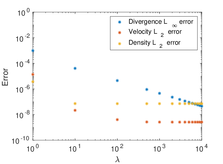
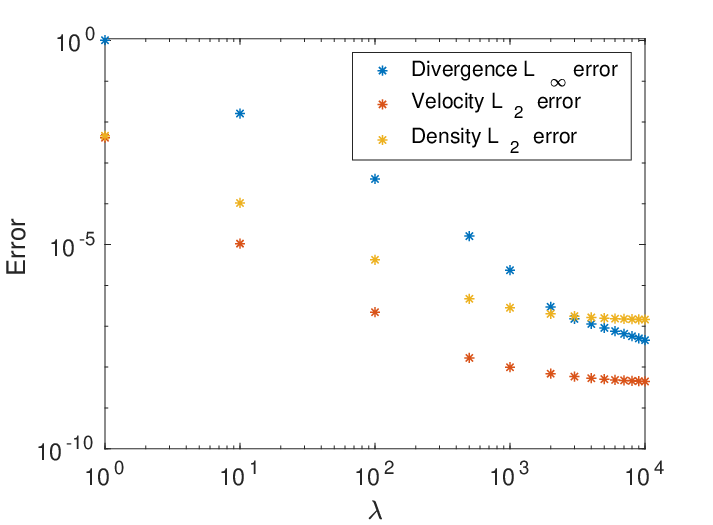
The , and errors are presented for all components. All the errors are computed using high-order quadrature and are relative, i.e. they are normalized with their corresponding norm. If the time derivatives are used as an initial condition we were able to obtain the expected high-order convergence rate using similar to Guermond and Minev 2019. However, when Algorithm 1 was used as initialization, we were unable to achieve this using a small . By increasing it was possible to obtain the correct convergence rate. In Section 6.2 we investigate how affects the error in more detail by doing a parameter sweep.
| dofs | rate | rate | rate | ||||
|---|---|---|---|---|---|---|---|
| Galerkin | 200 | 1.84E-03 | 0.00 | 2.11E-03 | 0.00 | 2.43E-03 | 0.00 |
| 386 | 7.41E-04 | 2.76 | 7.39E-04 | 3.19 | 6.68E-04 | 3.93 | |
| 794 | 1.83E-04 | 3.87 | 1.89E-04 | 3.79 | 2.06E-04 | 3.26 | |
| 3314 | 1.17E-05 | 3.85 | 1.36E-05 | 3.68 | 1.56E-05 | 3.61 | |
| 13184 | 7.03E-07 | 4.07 | 6.96E-07 | 4.31 | 6.46E-07 | 4.61 | |
| 52184 | 2.34E-08 | 4.95 | 2.89E-08 | 4.62 | 3.52E-08 | 4.23 |
| dofs | rate | rate | rate | ||||
|---|---|---|---|---|---|---|---|
| Galerkin | 100 | 2.37E-03 | 0.00 | 2.69E-03 | 0.00 | 3.32E-03 | 0.00 |
| 193 | 7.47E-04 | 3.51 | 8.47E-04 | 3.51 | 1.06E-03 | 3.48 | |
| 397 | 1.31E-04 | 4.83 | 1.49E-04 | 4.81 | 1.89E-04 | 4.77 | |
| 1657 | 3.03E-06 | 5.27 | 3.68E-06 | 5.19 | 5.40E-06 | 4.98 | |
| 6592 | 1.64E-07 | 4.23 | 1.91E-07 | 4.28 | 2.59E-07 | 4.40 | |
| 26092 | 1.18E-08 | 3.83 | 1.37E-08 | 3.83 | 1.85E-08 | 3.84 |
| dofs | rate | rate | rate | ||||
|---|---|---|---|---|---|---|---|
| Galerkin | 48 | 7.98E-02 | 0.00 | 7.79E-02 | 0.00 | 1.71E-01 | 0.00 |
| 91 | 2.68E-02 | 3.41 | 2.48E-02 | 3.58 | 2.38E-02 | 6.16 | |
| 184 | 6.81E-03 | 3.89 | 6.26E-03 | 3.92 | 5.63E-03 | 4.10 | |
| 751 | 7.53E-04 | 3.13 | 6.96E-04 | 3.12 | 7.08E-04 | 2.95 | |
| 2958 | 4.06E-05 | 4.26 | 3.81E-05 | 4.24 | 5.43E-05 | 3.75 | |
| 11652 | 1.59E-06 | 4.73 | 1.74E-06 | 4.50 | 3.79E-06 | 3.88 |
| dofs | rate | rate | rate | ||||
|---|---|---|---|---|---|---|---|
| Galerkin | 200 | 2.21E-06 | 0.00 | 2.40E-06 | 0.00 | 2.78E-06 | 0.00 |
| 386 | 3.49E-07 | 5.62 | 3.72E-07 | 5.67 | 4.62E-07 | 5.46 | |
| 794 | 7.53E-08 | 4.25 | 8.20E-08 | 4.19 | 1.05E-07 | 4.10 | |
| 3314 | 3.58E-09 | 4.26 | 3.85E-09 | 4.28 | 4.96E-09 | 4.28 | |
| 13184 | 2.23E-10 | 4.02 | 2.49E-10 | 3.97 | 3.43E-10 | 3.87 | |
| 52184 | 4.87E-10 | -1.13 | 5.01E-10 | -1.02 | 5.57E-10 | -0.71 |
| dofs | rate | rate | rate | ||||
|---|---|---|---|---|---|---|---|
| Galerkin | 100 | 8.50E-05 | 0.00 | 9.74E-05 | 0.00 | 1.58E-04 | 0.00 |
| 193 | 1.34E-05 | 5.61 | 1.53E-05 | 5.64 | 2.06E-05 | 6.20 | |
| 397 | 2.30E-06 | 4.90 | 2.59E-06 | 4.92 | 3.35E-06 | 5.04 | |
| 1657 | 1.19E-07 | 4.15 | 1.35E-07 | 4.14 | 1.83E-07 | 4.07 | |
| 6592 | 5.27E-09 | 4.51 | 6.23E-09 | 4.45 | 9.48E-09 | 4.28 | |
| 26092 | 4.63E-10 | 3.54 | 5.72E-10 | 3.47 | 9.85E-10 | 3.29 |
| dofs | rate | rate | rate | ||||
|---|---|---|---|---|---|---|---|
| Galerkin | 48 | 3.18E-03 | 0.00 | 4.89E-03 | 0.00 | 1.36E-02 | 0.00 |
| 91 | 1.38E-03 | 2.61 | 1.95E-03 | 2.87 | 5.09E-03 | 3.07 | |
| 184 | 4.49E-04 | 3.19 | 6.41E-04 | 3.16 | 1.55E-03 | 3.37 | |
| 751 | 5.51E-05 | 2.98 | 7.48E-05 | 3.05 | 2.18E-04 | 2.79 | |
| 2958 | 7.53E-06 | 2.90 | 9.94E-06 | 2.95 | 2.81E-05 | 2.99 | |
| 11652 | 9.54E-07 | 3.01 | 1.25E-06 | 3.02 | 3.03E-06 | 3.25 |
6.2 How effects different errors
In this section, we investigate how affects different errors of the solution. We use the same setup as in Section 6.1 with an unstructured mesh consisting of 1657 nodes. In Figure 1 the maximum divergence error over space and time, i.e. , is plotted against . Moreover, the relative error of the velocity and density at time is plotted against . Overall, the figure indicates that increasing decreases the divergence error and also decreases the error in density and velocity up to some threshold. Another important observation is that the Richardson initialization algorithm (Algorithm 1) requires a larger than when initial conditions for the time derivatives are used.
6.3 Loss of regularity
In this section, we investigate how the Taylor series time-stepping method handles problems with sharp gradients, i.e. when regularity of the solution is lost. The Taylor series method relies on computing time derivative correction terms to achieve high-order accuracy. Needing to compute time derivatives when the solution contains a discontinuity is problematic since the analytic time derivatives are infinitely large. If the discontinuity is regularized using a stabilization technique, computing the time derivatives might still be acceptable. We investigate this in Section 6.3.1 by considering a benchmark problem where regularity is lost.
We emphasize that there exist many stabilization methods which can be applied to the first-order method from Section 3. Some options include entropy viscosity [28, 42, 27], residual viscosity [41, 48, 36, 38, 15], first-order viscosity, Galerkin least-squares [29] and so on. Stabilizing the time derivative updates from Section 4 is an entirely different matter since the analytic time derivatives are unbounded in the presence of a discontinuity.
We choose to stabilize the method and its time derivative updates using -viscosity, which is one of the most robust spatial stabilizations possible. Our aim is not to achieve an accurate result since the results will be overly diffusive and only first-order accurate in space. Instead, our aim is simply to try to stabilize the method and illustrate that even with this very diffuse stabilization the Taylor series method is not suited for problems of this kind. We impose -viscosity by setting and where is a constant, see Sections 4.2.1 and 4.2.2.
Remark 6.1.
For a hyperbolic problem in one space dimension using finite elements in space and explicit Euler in time, it can be shown that scaling the artificial viscosity coefficient as leads to the classical first-order upwind scheme which is a convergent scheme [33].
Remark 6.2.
A more suitable time-stepping method would be a method that allows for loss of regularity. Finding such a scheme in the context of high-order artificial compressibility is an open question. We suspect that the defect correction time-stepping approach from [20, Sec 5.2] suffers from a similar problem as the Taylor series method does. A viable alternative would be the modified high-order BDF scheme proposed in [20, Sec 5.1]. The downside would be that the scheme would lose its A-stability. One could also consider using a Lagrange-Galerkin approach. The Lagrange-Galerkin method discretizes the total derivative (the convective part of the equations) backward in time along the characteristic curves and has been successfully applied to hyperbolic problems [13] and incompressible flow [6, 5]. Investigating if this time-stepping approach is amenable to high-order artificial compressibility would certainly be an interesting research topic.
6.3.1 2D Rayleigh-Taylor instability
As a test problem where regularity is lost, we consider the Rayleigh-Taylor instability in 2D. The Rayleigh-Taylor instability occurs when a fluid accelerates into another fluid with a different density. The classical setup is that a heavier fluid is supported by a lighter fluid in a gravitational field. Any small perturbation to the system forces it out of equilibrium since the initial equilibrium state is unstable. We follow the same setup as Guermond and Salgado 2009. The solution is computed in a rectangular domain . The density jump is initially regularized using a hyperbolic tangent function and is given by
| (44) |
where . Slip boundary conditions are enforced at the boundaries. The characteristic velocity scale is set to which gives the Reynolds number . The following parameters are used: , , , , , , , , CFL = 0.5, , . A sufficiently large value of is set to ensure that divergence errors are negligible, see Section 6.2 for more details. We use a structured mesh containing 45676 nodes, which later is uniformly refined two times.
In Figures 2-4 we present the time evolution of the computed density field for , respectively, in the time-scale of Tryggvason (). Overall, the results are in agreement with the result obtained by Guermond and Salgado 2009 where a second-order accurate Taylor-Hood finite element method was used. Since -viscosity was used as stabilization the results presented here are very diffused. As a comparison we present results with the first-order algorithm from Section 3 in Figure 5. Overall, the results of the first-order algorithm is completely identical to the Taylor series method.
In Figures 6-8 the computed third time derivative of the density is presented. We observe that the magnitude of the solution is increased when the grid is refined. The reason why the time derivative increases is that the gradient of the solution grows upon grid refinement. We infer that the time derivative will continue to grow without bound as the grid is refined. We, therefore, conclude that the Taylor series method is unsuitable for problems where the regularity of the solution is lost. A more accurate and sharp stabilization procedure will exaggerate this issue.


Remark 6.3.
Since for this problem, setting will lead to slightly more diffusive results than than . Qualitatively, the results are similar in the sense that the computed time derivatives grow without bound upon grid refinement.
7 Conclusion and further work
A fourth-order accurate finite element method for variable density incompressible flow is proposed. The method uses artificial compressibility to impose the divergence-free constraint following the ideas presented by Guermond and Minev 2019 which we have extended to variable density. In space continuous finite elements are used and in time the Taylor series time-stepping method is used. If initial conditions for the time derivatives are available, the proposed method is high-order accurate using the penalty parameter , which makes the condition number of the resulting linear systems suitable for large-scale applications. If these initial conditions are not available, a Richardson initialization procedure can be used which requires a larger .
We also illustrate that the Taylor series time-stepping method is not suitable when the regularity of the solution is lost by solving the Rayleigh-Taylor instability in 2D. The reason for this is that when the grid is refined, the time derivatives increase in magnitude without bound. Our current work is aimed at overcoming this problem, and the development of a reliable high-order finite element approximation for variable density flow will be reported in our future publication.
Acknowledgments
We thank the anonymous reviewers whose comments helped improve the quality of this manuscript. The computations were enabled by resources in project SNIC 2022/22-428 provided by the Swedish National Infrastructure for Computing (SNIC) at UPPMAX, partially funded by the Swedish Research Council through grant agreement no. 2018-05973. The first author was partly supported by the Center for Interdisciplinary Mathematics, Uppsala University.
8 Appendix
In this section we present estimates for the first-order scheme from Section 2.2. We denote as the -norm. To make the analysis simpler we assume that , which will make many boundary terms resulting from integration by parts disappear. Similarly, we set .
8.1 First order scheme, density update
We take the density update (5) and and discretize the flux skew-symmetrically. That gives us the following scheme
| (45) |
We now present an estimate for this scheme. The result and proof are standard and can be found elsewhere (for example [24]), but we recap it below for completeness.
Proposition 8.1.
The density update (45) satisfies the following -estimate
| (46) |
Proof.
Multiplying (45) with , integrating over and using yields
| (47) |
For the advection term we have
| (48) |
where integration by parts was used in the last equality. We then have the desired estimate.
∎
8.2 First order scheme, velocity form
In this section, we present estimates of the momentum update. We take the first-order momentum update (6)-(7), discretize the advection term skew-symmetrically and semi-implicitly and shift the density on the time derivative to . To the best of the authors’ knowledge, these modifications are necessary to obtain an -estimate. The shifted density will unfortunately make high-order extensions (like those presented in this work) harder since it will limit the order of accuracy in time to first-order accuracy. There have been some attempts at overcoming this issue for BDF2 based time-stepping by Guermond and Salgado 2011, but it remains an open question. The scheme that we consider is the following
| (49) |
| (50) |
We follow a very similar proof technique as Guermond and Salgado 2009 did for variable density and as Chen et al. 2019 did for artificial compressibility.
Proposition 8.2.
Proof.
We multiply (49) with and integrate over the domain. Integration by parts is performed on the diffusion term and the identity is applied to the time derivative term leading to
| (52) |
Next, we take the density update (45) and multiply with . Integrating over the domain and integrating by parts then gives
| (53) |
Adding (52) and (53) and performing integration by parts on the pressure term yields
| (54) |
To deal with the pressure term we first multiply the pressure update (50) with , integrate over the domain and apply the identity . Performing these steps gives
| (55) |
∎
References
- Alnaes et al. [2015] M. Alnaes, J. Blechta, J. Hake, A. Johansson, B. Kehlet, A. Logg, C. Richardson, J. Ring, M. Rognes, and G. Wells. The FEniCS project version 1.5. Arch. Numer. Softw., 3:9–23, 01 2015. doi: 10.11588/ans.2015.100.20553. URL https://doi.org/10.11588/ans.2015.100.20553.
- Alrashed [2015] F. S. A. Alrashed. Parallel multiphase Navier-Stokes solver. ProQuest LLC, Ann Arbor, MI, 2015. ISBN 978-1339-17274-3. URL http://gateway.proquest.com/openurl?url_ver=Z39.88-2004&rft_val_fmt=info:ofi/fmt:kev:mtx:dissertation&res_dat=xri:pqm&rft_dat=xri:pqdiss:3730933. Thesis (Ph.D.)–Texas A&M University.
- Axelsson et al. [2015] O. Axelsson, X. He, and M. Neytcheva. Numerical solution of the time-dependent Navier-Stokes equation for variable density–variable viscosity. Part I. Math. Model. Anal., 20(2):232–260, 2015. ISSN 1392-6292. doi: 10.3846/13926292.2015.1021395. URL https://doi.org/10.3846/13926292.2015.1021395.
- Bassi et al. [2018] F. Bassi, F. Massa, L. Botti, and A. Colombo. Artificial compressibility Godunov fluxes for variable density incompressible flows. Comput. & Fluids, 169:186–200, 2018. ISSN 0045-7930. doi: 10.1016/j.compfluid.2017.09.010. URL https://doi.org/10.1016/j.compfluid.2017.09.010.
- Bermejo and Saavedra [2016] R. Bermejo and L. Saavedra. Lagrange-Galerkin methods for the incompressible Navier-Stokes equations: a review. Commun. Appl. Ind. Math., 7(3):26–52, 2016. doi: 10.1515/caim-2016-0021. URL https://doi.org/10.1515/caim-2016-0021.
- Bermejo and Saavedra [2018] R. Bermejo and L. Saavedra. Local projection stabilized Lagrange-Galerkin methods for Navier-Stokes equations at high Reynolds numbers. SeMA J., 75(4):607–627, 2018. ISSN 2254-3902. doi: 10.1007/s40324-018-0155-3. URL https://doi.org/10.1007/s40324-018-0155-3.
- Bowers et al. [2014] A. L. Bowers, S. Le Borne, and L. G. Rebholz. Error analysis and iterative solvers for Navier-Stokes projection methods with standard and sparse grad-div stabilization. Comput. Methods Appl. Mech. Engrg., 275:1–19, 2014. ISSN 0045-7825. doi: 10.1016/j.cma.2014.02.021. URL https://doi.org/10.1016/j.cma.2014.02.021.
- Case et al. [2011] M. A. Case, V. J. Ervin, A. Linke, and L. G. Rebholz. A connection between Scott-Vogelius and grad-div stabilized Taylor-Hood FE approximations of the Navier-Stokes equations. SIAM J. Numer. Anal., 49(4):1461–1481, 2011. ISSN 0036-1429. doi: 10.1137/100794250. URL https://doi.org/10.1137/100794250.
- Charnyi et al. [2017] S. Charnyi, T. Heister, M. A. Olshanskii, and L. G. Rebholz. On conservation laws of Navier-Stokes Galerkin discretizations. J. Comput. Phys., 337:289–308, 2017. ISSN 0021-9991. doi: 10.1016/j.jcp.2017.02.039. URL https://doi.org/10.1016/j.jcp.2017.02.039.
- Chen et al. [2020] H. Chen, J. Mao, and J. Shen. Error estimate of gauge-Uzawa methods for incompressible flows with variable density. J. Comput. Appl. Math., 364:112321, 14, 2020. ISSN 0377-0427. doi: 10.1016/j.cam.2019.06.037. URL https://doi.org/10.1016/j.cam.2019.06.037.
- Chen et al. [2019] R. M. Chen, W. Layton, and M. McLaughlin. Analysis of variable-step/non-autonomous artificial compression methods. J. Math. Fluid Mech., 21(2):Paper No. 30, 20, 2019. ISSN 1422-6928. doi: 10.1007/s00021-019-0429-2. URL https://doi.org/10.1007/s00021-019-0429-2.
- Chorin [1967] A. J. Chorin. A numerical method for solving incompressible viscous flow problems. J. Comput. Phys., 2(1):12–26, 1967. ISSN 0021-9991. doi: 10.1016/0021-9991(67)90037-X. URL https://doi.org/10.1016/0021-9991(67)90037-X.
- Colera et al. [2021] M. Colera, J. Carpio, and R. Bermejo. A nearly-conservative, high-order, forward Lagrange-Galerkin method for the resolution of scalar hyperbolic conservation laws. Comput. Methods Appl. Mech. Engrg., 376:Paper No. 113654, 28, 2021. ISSN 0045-7825. doi: 10.1016/j.cma.2020.113654. URL https://doi.org/10.1016/j.cma.2020.113654.
- Cox et al. [2016] C. Cox, C. Liang, and M. W. Plesniak. A high-order solver for unsteady incompressible Navier-Stokes equations using the flux reconstruction method on unstructured grids with implicit dual time stepping. J. Comput. Phys., 314:414–435, 2016. ISSN 0021-9991. doi: 10.1016/j.jcp.2016.03.016. URL https://doi.org/10.1016/j.jcp.2016.03.016.
- Dao and Nazarov [2022] T. A. Dao and M. Nazarov. A High-Order Residual-Based Viscosity Finite Element Method for the Ideal MHD Equations. J. Sci. Comput., 92(3):Paper No. 77, 2022. ISSN 0885-7474. doi: 10.1007/s10915-022-01918-4. URL https://doi.org/10.1007/s10915-022-01918-4.
- de Frutos et al. [2018] J. de Frutos, B. García-Archilla, V. John, and J. Novo. Analysis of the grad-div stabilization for the time-dependent Navier-Stokes equations with inf-sup stable finite elements. Adv. Comput. Math., 44(1):195–225, 2018. ISSN 1019-7168. doi: 10.1007/s10444-017-9540-1. URL https://doi.org/10.1007/s10444-017-9540-1.
- DeCaria et al. [2017] V. DeCaria, W. Layton, and M. McLaughlin. A conservative, second order, unconditionally stable artificial compression method. Comput. Methods Appl. Mech. Engrg., 325:733–747, 2017. ISSN 0045-7825. doi: 10.1016/j.cma.2017.07.033. URL https://doi.org/10.1016/j.cma.2017.07.033.
- DeCaria et al. [2019] V. DeCaria, W. Layton, and M. McLaughlin. An analysis of the Robert-Asselin time filter for the correction of nonphysical acoustics in an artificial compression method. Numer. Methods Partial Differential Equations, 35(3):916–935, 2019. ISSN 0749-159X. doi: 10.1002/num.22331. URL https://doi.org/10.1002/num.22331.
- DeCaria et al. [2020] V. DeCaria, T. Iliescu, W. Layton, M. McLaughlin, and M. Schneier. An artificial compression reduced order model. SIAM J. Numer. Anal., 58(1):565–589, 2020. ISSN 0036-1429. doi: 10.1137/19M1246444. URL https://doi.org/10.1137/19M1246444.
- Guermond and Minev [2015] J.-L. Guermond and P. Minev. High-order time stepping for the incompressible Navier-Stokes equations. SIAM J. Sci. Comput., 37(6):A2656–A2681, 2015. ISSN 1064-8275. doi: 10.1137/140975231. URL https://doi.org/10.1137/140975231.
- Guermond and Minev [2019] J.-L. Guermond and P. Minev. High-order adaptive time stepping for the incompressible Navier-Stokes equations. SIAM J. Sci. Comput., 41(2):A770–A788, 2019. ISSN 1064-8275. doi: 10.1137/18M1209301. URL https://doi.org/10.1137/18M1209301.
- Guermond and Minev [2017] J.-L. Guermond and P. D. Minev. High-order time stepping for the Navier-Stokes equations with minimal computational complexity. J. Comput. Appl. Math., 310:92–103, 2017. ISSN 0377-0427. doi: 10.1016/j.cam.2016.04.033. URL https://doi.org/10.1016/j.cam.2016.04.033.
- Guermond and Pasquetti [2013] J.-L. Guermond and R. Pasquetti. A correction technique for the dispersive effects of mass lumping for transport problems. Comput. Methods Appl. Mech. Engrg., 253:186–198, 2013. ISSN 0045-7825. doi: 10.1016/j.cma.2012.08.011. URL https://doi.org/10.1016/j.cma.2012.08.011.
- Guermond and Salgado [2009] J.-L. Guermond and A. Salgado. A splitting method for incompressible flows with variable density based on a pressure Poisson equation. J. Comput. Phys., 228(8):2834–2846, 2009. ISSN 0021-9991. doi: 10.1016/j.jcp.2008.12.036. URL http://dx.doi.org/10.1016/j.jcp.2008.12.036.
- Guermond and Salgado [2011] J.-L. Guermond and A. J. Salgado. Error analysis of a fractional time-stepping technique for incompressible flows with variable density. SIAM J. Numer. Anal., 49(3):917–944, 2011. ISSN 0036-1429. doi: 10.1137/090768758. URL http://dx.doi.org/10.1137/090768758.
- Guermond et al. [2006] J. L. Guermond, P. Minev, and J. Shen. An overview of projection methods for incompressible flows. Comput. Methods Appl. Mech. Engrg., 195(44-47):6011–6045, 2006. ISSN 0045-7825. doi: 10.1016/j.cma.2005.10.010. URL https://doi.org/10.1016/j.cma.2005.10.010.
- Guermond et al. [2011a] J.-L. Guermond, M. Nazarov, and B. Popov. Implementation of the entropy viscosity method. Technical Report 4015, KTH, Numerical Analysis, NA, 2011a. QC 20110720.
- Guermond et al. [2011b] J.-L. Guermond, R. Pasquetti, and B. Popov. Entropy viscosity method for nonlinear conservation laws. J. Comput. Phys., 230(11):4248–4267, 2011b. ISSN 0021-9991. doi: 10.1016/j.jcp.2010.11.043. URL https://doi.org/10.1016/j.jcp.2010.11.043.
- Hughes et al. [1989] T. J. R. Hughes, L. P. Franca, and G. M. Hulbert. A new finite element formulation for computational fluid dynamics. VIII. The Galerkin/least-squares method for advective-diffusive equations. Comput. Methods Appl. Mech. Engrg., 73(2):173–189, 1989. ISSN 0045-7825. doi: 10.1016/0045-7825(89)90111-4. URL https://doi.org/10.1016/0045-7825(89)90111-4.
- Jenkins et al. [2014] E. W. Jenkins, V. John, A. Linke, and L. G. Rebholz. On the parameter choice in grad-div stabilization for the Stokes equations. Adv. Comput. Math., 40(2):491–516, 2014. ISSN 1019-7168. doi: 10.1007/s10444-013-9316-1. URL https://doi.org/10.1007/s10444-013-9316-1.
- John and Kindl [2010] V. John and A. Kindl. Numerical studies of finite element variational multiscale methods for turbulent flow simulations. Comput. Methods Appl. Mech. Engrg., 199(13-16):841–852, 2010. ISSN 0045-7825. doi: 10.1016/j.cma.2009.01.010. URL https://doi.org/10.1016/j.cma.2009.01.010.
- Kronbichler et al. [2018] M. Kronbichler, A. Diagne, and H. Holmgren. A fast massively parallel two-phase flow solver for microfluidic chip simulation. Int. J. of High Perform. Comput. Appl., 32(2):266–287, 2018. doi: 10.1177/1094342016671790. URL https://doi.org/10.1177/1094342016671790.
- Lax [1954] P. D. Lax. Weak solutions of nonlinear hyperbolic equations and their numerical computation. Comm. Pure Appl. Math., 7:159–193, 1954. ISSN 0010-3640. doi: 10.1002/cpa.3160070112. URL https://doi.org/10.1002/cpa.3160070112.
- Layton and McLaughlin [2020] W. Layton and M. McLaughlin. Doubly-adaptive artificial compression methods for incompressible flow. J. Numer. Math., 28(3):179–196, 2020. ISSN 1570-2820. doi: 10.1515/jnma-2019-0015. URL https://doi.org/10.1515/jnma-2019-0015.
- Linke and Rebholz [2013] A. Linke and L. G. Rebholz. On a reduced sparsity stabilization of grad-div type for incompressible flow problems. Comput. Methods Appl. Mech. Engrg., 261/262:142–153, 2013. ISSN 0045-7825. doi: 10.1016/j.cma.2013.04.005. URL https://doi.org/10.1016/j.cma.2013.04.005.
- Lu et al. [2019] L. Lu, M. Nazarov, and P. Fischer. Nonlinear artificial viscosity for spectral element methods. C. R. Math. Acad. Sci. Paris, 357(7):646–654, 2019. ISSN 1631-073X. doi: 10.1016/j.crma.2019.07.006. URL https://doi.org/10.1016/j.crma.2019.07.006.
- Manzanero et al. [2020] J. Manzanero, G. Rubio, D. A. Kopriva, E. Ferrer, and E. Valero. An entropy-stable discontinuous Galerkin approximation for the incompressible Navier-Stokes equations with variable density and artificial compressibility. J. Comput. Phys., 408:109241, 32, 2020. ISSN 0021-9991. doi: 10.1016/j.jcp.2020.109241. URL https://doi.org/10.1016/j.jcp.2020.109241.
- Marras et al. [2015] S. Marras, M. Nazarov, and F. X. Giraldo. Stabilized high-order Galerkin methods based on a parameter-free dynamic SGS model for LES. J. Comput. Phys., 301:77–101, 2015. ISSN 0021-9991. doi: 10.1016/j.jcp.2015.07.034. URL https://doi.org/10.1016/j.jcp.2015.07.034.
- Milani [2020] R. Milani. Compatible Discrete Operator schemes for the unsteady incompressible Navier–Stokes equations. Theses, Université Paris-Est, Dec. 2020. URL https://tel.archives-ouvertes.fr/tel-03080530.
- Minev and Vabishchevich [2018] P. Minev and P. N. Vabishchevich. Splitting schemes for unsteady problems involving the grad-div operator. Appl. Numer. Math., 124:130–139, 2018. ISSN 0168-9274. doi: 10.1016/j.apnum.2017.10.005. URL https://doi.org/10.1016/j.apnum.2017.10.005.
- Nazarov and Hoffman [2013] M. Nazarov and J. Hoffman. Residual-based artificial viscosity for simulation of turbulent compressible flow using adaptive finite element methods. Internat. J. Numer. Methods Fluids, 71(3):339–357, 2013. ISSN 0271-2091. doi: 10.1002/fld.3663. URL http://dx.doi.org/10.1002/fld.3663.
- Nazarov and Larcher [2017] M. Nazarov and A. Larcher. Numerical investigation of a viscous regularization of the Euler equations by entropy viscosity. Comput. Methods Appl. Mech. Engrg., 317:128–152, 2017. ISSN 0045-7825. doi: 10.1016/j.cma.2016.12.010. URL https://doi.org/10.1016/j.cma.2016.12.010.
- Olshanskii et al. [2009] M. Olshanskii, G. Lube, T. Heister, and J. Löwe. Grad-div stabilization and subgrid pressure models for the incompressible Navier-Stokes equations. Comput. Methods Appl. Mech. Engrg., 198(49-52):3975–3988, 2009. ISSN 0045-7825. doi: 10.1016/j.cma.2009.09.005. URL https://doi.org/10.1016/j.cma.2009.09.005.
- Olshanskii and Reusken [2004] M. A. Olshanskii and A. Reusken. Grad-div stabilization for Stokes equations. Math. Comp., 73(248):1699–1718, 2004. ISSN 0025-5718. doi: 10.1090/S0025-5718-03-01629-6. URL https://doi.org/10.1090/S0025-5718-03-01629-6.
- Pyo and Shen [2007] J.-H. Pyo and J. Shen. Gauge-Uzawa methods for incompressible flows with variable density. J. Comput. Phys., 221(1):181–197, 2007. ISSN 0021-9991. doi: 10.1016/j.jcp.2006.06.013. URL https://doi.org/10.1016/j.jcp.2006.06.013.
- Röhe and Lube [2010] L. Röhe and G. Lube. Analysis of a variational multiscale method for large-eddy simulation and its application to homogeneous isotropic turbulence. Comput. Methods Appl. Mech. Engrg., 199(37-40):2331–2342, 2010. ISSN 0045-7825. doi: 10.1016/j.cma.2010.02.015. URL https://doi.org/10.1016/j.cma.2010.02.015.
- Shen [1996] J. Shen. On a new pseudocompressibility method for the incompressible Navier-Stokes equations. Appl. Numer. Math., 21(1):71–90, 1996. ISSN 0168-9274. doi: 10.1016/0168-9274(95)00132-8. URL https://doi.org/10.1016/0168-9274(95)00132-8.
- Stiernström et al. [2021] V. Stiernström, L. Lundgren, M. Nazarov, and K. Mattsson. A residual-based artificial viscosity finite difference method for scalar conservation laws. Journal of Computational Physics, page 110100, 2021. ISSN 0021-9991. doi: https://doi.org/10.1016/j.jcp.2020.110100. URL http://www.sciencedirect.com/science/article/pii/S0021999120308743.
- Temam [1968] R. Temam. Une méthode d’approximation de la solution des équations de Navier-Stokes. Bull. Soc. Math. France, 96:115–152, 1968. ISSN 0037-9484. URL http://www.numdam.org/item?id=BSMF_1968__96__115_0.
- Wu et al. [2017] J. Wu, J. Shen, and X. Feng. Unconditionally stable gauge-Uzawa finite element schemes for incompressible natural convection problems with variable density. J. Comput. Phys., 348:776–789, 2017. ISSN 0021-9991. doi: 10.1016/j.jcp.2017.07.045. URL https://doi.org/10.1016/j.jcp.2017.07.045.
- Yang et al. [2016] L. Yang, S. Badia, and R. Codina. A pseudo-compressible variational multiscale solver for turbulent incompressible flows. Comput. Mech., 58(6):1051–1069, 2016. ISSN 0178-7675. doi: 10.1007/s00466-016-1332-9. URL https://doi.org/10.1007/s00466-016-1332-9.