Quintessence from a state space perspective
Abstract
We use dynamical systems methods to study quintessence models in a spatially flat and isotropic spacetime with matter and a scalar field with potentials for which is bounded, thereby going beyond the exponential potential for which is constant. The scalar field equation of state parameter plays a central role when comparing quintessence models with observations, but with the dynamical systems used to date is an indeterminate, discontinuous, function on the state space in the asymptotically matter dominated regime. Our first main result is the introduction of new variables that lead to a regular dynamical system on a bounded three-dimensional state space on which is a regular function. The solution trajectories in the state space then provide a visualization of different types of quintessence evolution, and how initial conditions affect the transition between the matter and scalar field dominated epochs; this is complemented by graphs , where is the -fold time, which enables characterizing different types of quintessence evolution.
1 Introduction
In 1998 observations of type Ia supernovae indicated that the Universe is undergoing late-time acceleration [1, 2]. Within the framework of General Relativity this cosmic acceleration implies that there exists an exotic energy component in the Universe, called dark energy, with an equation of state satisfying . Observational constraints on , assumed to be constant, provided by the cosmic microwave background and the large-scale structure of the Universe continue to tighten and are typically of order (see, e.g., Suzuki et al. (2012) [3], section 5, Ade et al. (2016) [4], section 5, and more briefly, Chiba et al. (2013) [5], the introduction and section III). The simplest hypothesis compatible with these observations is that the dark energy is a cosmological constant with exactly equal to , and that the Universe can be described by the CDM model, which is currently viewed as the standard model of cosmology. Although this simple model is in surprisingly good agreement with observations, it is still possible that the equation of state of dark energy is not constant but instead depends on time in a way that is compatible with observations. For this reason other candidates for dark energy have been extensively investigated. The simplest of these is a dynamical canonical scalar field , minimally coupled to gravity and with a potential , referred to as quintessence, the fifth element of the current matter content in the Universe, after baryons, dark matter, radiation, and neutrinos, Caldwell et al. (1998) [6].
The quintessence mechanism generating the present acceleration of the Universe resembles that of inflation in the very early Universe, i.e., a canonical scalar field rolling slowly down a slowly varying potential , although the energy scale of the quintessence potential is tiny compared to that of the inflaton potential. Furthermore, in contrast to inflation, quintessence dynamics also involve non-relativistic matter (baryons and cold dark matter). Loosely speaking, the dynamics of the quintessence field is governed by its equation of state parameter , with observations requiring that at the present time is sufficiently close to . We note that the CDM model can be viewed as a limiting quintessence model with constant potential and a constant scalar field, which results in . It is expected that upcoming large scale structure surveys will impose increasingly tight constraints on the value of and its time rate of change at the present time (Akrami et al. (2020) [7], see the abstract).
In 1998 it was shown by Copeland et al. [8] that for a model with a single matter component with a linear equation of state, and with the simplest type of potential, the exponential potential, the governing equations could be formulated as a dynamical system on a two dimensional state space.11 1 A dynamical system is a system of differential equations of the form where describes the state space, is a vector field on and ′ denotes the derivative with respect to time. Dynamical systems methods were first used in cosmology in 1971 by Collins [9], using two-dimensional systems to study anisotropic Bianchi models. This early work has subsequently been extended by many researchers to systems in higher dimensions, see e.g. [10, 11, 12] and references therein. This enabled cosmologists to apply standard techniques of dynamical systems theory to describe the evolution of these simple quintessence models. For more general potentials, however, one needs a three-dimensional autonomous system of equations in order to describe the extra degree of freedom in the scalar field.
In this paper we consider potentials such that is bounded, the simplest being the exponential potential for which is constant. To study models with varying , Alho and Uggla (2015) [13] introduced a regular dynamical system on a bounded three-dimensional state space, where two of the variables were closely related to those used by Copeland et al. [8] for an exponential potential. As will be shown in a future paper, this system is effective for deriving new simple and accurate approximations of scalar field quantities such as the equation of state parameter and the Hubble-normalized scalar field energy density , thereby simplifying comparisons with observational data. However, it has the drawback that is indeterminate in the asymptotically matter dominated regime where is zero. We therefore introduce two new variables, closely related to and , that lead to a new regular dynamical system on a bounded three-dimensional state space that avoids the indeterminacy problem, which allows us to define and study various types of quintessence.
According to Tsujikawa (2013) [14] there are three types of quintessence in the literature: thawing, scaling freezing, and tracking freezing quintessence. The concepts of thawing and freezing were defined by Caldwell and Linder (2005) [15] as follows: thawing is characterized by where subsequently grows, i.e. , while and holds for freezing.22 2 Here ′ denotes the derivative with respect to -fold time , see equation (6). In this paper we will refine the classification in [14] and in addition to thawing, scaling freezing, and tracking freezing quintessence also define freezing quintessence, scaling oscillatory quintessence and oscillatory quintessence.
The outline of the paper is as follows. In the next section we derive the new dynamical system, assuming a potential with bounded . In section 3 we describe global properties of the state space and discuss invariant boundary sets, fixed points and asymptotic behaviour. Section 4 contains a discussion of various types of quintessence from a state space perspective using the new dynamical system. The following section uses the double-exponential potential as a simple example to illustrate the different types of quintessence by means of state space pictures and complementary graphs of and , i.e. the ratio of the Hubble variable for quintessence and CDM. Section 6 summarizes our results, illustrating our quintessence classification scheme with examples from the literature, and concludes with some comments about future developments.
2 Derivation of the new dynamical system
Consider a spatially flat and isotropic Friedmann-Lemaître-Robertson-Walker (FLRW) spacetime,
| (1) |
where is the cosmological scale factor. The source consists of matter with an energy density and pressure , which represents cold dark matter33 3 This simple model is useful for describing the transition from an epoch of matter domination to an epoch in which the scalar field is dominant. A more realistic model is provided by a two component source with matter and radiation, in which there is an epoch of radiation domination preceding the epoch of matter domination, see the end of section 4.1. Although generalizing the discussion to include radiation is straightforward, it leads to a four-dimensional state space instead of the present three-dimensional one, which complicates visualization. For simplicity and pedagogically illustrative reasons we therefore neglect radiation in this paper, although we will include it in future work. and a minimally coupled scalar field, , with a potential , which results in
| (2) |
where an overdot represents the derivative with respect to the cosmic proper time . The Raychaudhuri equation, the Friedmann equation, the (non-linear) Klein-Gordon equation, and the energy conservation law for matter with zero pressure, can be written as44 4 We use units so that and , where is the speed of light and is the gravitational constant.
| (3a) | ||||
| (3b) | ||||
| (3c) | ||||
| (3d) | ||||
where the Hubble variable is defined by , and the total energy density and pressure are given by
| (4) |
Since implies that in (3b), it follows that for initially expanding models.
To obtain useful dynamical systems, we first introduce the following dimensionless and bounded Hubble-normalized quantities:55 5 The variable was first introduced by Coley et al. (1997) [16] and Copeland et al. (1998) [8], whose is . Since then, (or ) is now commonly used to describe scalar fields in cosmology, see, e.g., Urena-Lopez (2012) [17], equation (2.3), Tsujikawa (2013) [14], equation (16) and Alho and Uggla (2015) [13], equation (8). The reason for using the notation for the kernel is because plays a role that is similar to Hubble-normalized shear, which is typically denoted with the kernel , see e.g. [10].
| (5a) | ||||
| (5b) | ||||
| (5c) | ||||
A ′ henceforth denotes the derivative with respect to -fold time
| (6) |
where refers to the present time, and . The definition (6) implies that and when and , respectively.
To obtain dimensionless dynamical systems we replace the cosmic proper time with the dimensionless -fold time using the following relations:
| (7) |
where
| (8) |
is the deceleration parameter.
We consider potentials for which
| (9a) | |||
| is a regular bounded function for all with limits | |||
| (9b) | |||
i.e., we consider asymptotically exponential (or constant, when ) potentials, since . Depending on the form of the potential we choose a regular bounded increasing (and hence invertible) function which satisfies
| (10) |
For a fairly wide class of simple potentials a suitable choice of is66 6 More generally the choice of should be adapted to the properties of , especially the asymptotic ones; for some examples, see Alho and Uggla (2015) [13].
| (11) |
where the choice of the constants and depends on the potential. Since is assumed to be a bounded and sufficiently differentiable function of and the function is invertible we can define (with a slight abuse of notation) , where is the inverse function of . It follows from (9b) and (10) that
| (12) |
Using as the state vector and as the time variable, the definitions (5), (8), and the equations in (3) result in the following dynamical system:77 7 This system was used by Alho and Uggla (2015) [13], equation (9), with variables , where while corresponds to .
| (13a) | ||||
| (13b) | ||||
| (13c) | ||||
| where | ||||
| (13d) | ||||
| (13e) | ||||
The state space is bounded and described by the inequalities:
| (14) |
which follow from and . Specifying the scalar field potential and thereby results in that (13) forms a regular dynamical system on a bounded state space for a wide class of scalar field models.88 8 That the dynamical system is regular means that the functions in the vector field on the right side are bounded and sufficiently differentiable on the state space. If a dynamical system is regular one can use standard techniques to investigate the stability of the fixed points (singular points, critical points, equilibrium points). A bounded state space has the advantage that a regular dynamical system has future and past attractors in the state space and that one can describe the global properties of the solutions. Due to (13), obeys the auxiliary equation
| (15) |
from which it follows that is an invariant boundary set, as is due to (13c).
The inequalities in (14) imply that and are bounded above by . The state space can be visualized as a bounded three-dimensional set with rectangular base , , , bounded above by the tent-like surface , and with vertical ends , see Figure 1(a).
Before continuing we digress to place the dynamical system (13) in a historical context. If is constant, which means that the potential is exponential, , equations (13b) and (13c) form a two-dimensional dynamical system that is closely related to the widely used system introduced by Copeland et al. (1998) [8] in which the dynamical variables are99 9 See their equation (5) and our equation (5). To obtain (13) from their equations, use and as the dynamical variable. and . To go beyond the exponential potential, is sometimes added as a dynamical variable, whose evolution equation is given by
| (16) |
The resulting system is not autonomous due to the dependence of and on . However, if is monotone and hence invertible, i.e. we can write it follows that is a function of : . For this restricted class of potentials the resulting system using as a variable is autonomous.1010 10 See Bahamonde et al. (2018) [12], page 40, equations (4.53)-(4.56), and references given there. In particular, Table 10 in [12] gives a list of potentials for which can be written as a function of , but for most of these potentials is unbounded. This system of equations has been used, e.g., by Fang et al. (2009) [18], see their equations (5)-(7), and Urena-Lopez (2012) [17], equations (2.4) and (2.8).
In setting up the dynamical system (13) we have avoided imposing this restriction on the potential by initially simply adding as a variable, following Nunes and Mimoso (2000) [19] and Alho and Uggla (2015) [13], with the definition (5a) of acting as the evolution equation for , and then replacing with a suitable bounded variable .
We next introduce two key quantities associated with the scalar field: the Hubble-normalized scalar field energy density and the equation of state parameter ,
| (17a) | ||||
| (17b) | ||||
It follows that where when , , and when , . These quantities, while not directly observable, play an important role in determining the restrictions observations place on quintessence evolution. It follows from (17), however, that is indeterminate when , which is a drawback of using (13) as evolution equations. To avoid this problem one could consider using and as dynamical variables. It follows from (13) that the evolution equations for and are given by
| (18a) | ||||
| (18b) | ||||
This is not a regular system due to the appearance of which has to be obtained from (17b).1111 11 Bahamonde et al. (2018) [12], page 26, comment that although and are useful when comparing with observational data, there are mathematical difficulties in using them as dynamical variables. This appears to be a dead-end as regards obtaining regular evolution equations in a state space on which is well-defined. However, we have noticed that the system (18) can be made regular by writing
| (19) |
and specifying that has the same sign as and that , which with (17b) implies the following key relations:1212 12 The transformation (20) maps the two-dimensional boundary set of the ‘box state space’ onto the one-dimensional line of fixed points , , in the ‘tent state space’, and is thereby not one-to-one, see Figure 1. The factor in the definition of leads to the simple relation while the factor in the definition of avoids a factor in the equations.
| (20a) | ||||||
| (20b) | ||||||
It follows that the system (13) assumes the form
| (21a) | ||||
| (21b) | ||||
| (21c) | ||||
where is the constant in the definition (11) of . The state space is bounded and is described by the following inequalities:
| (22) |
Once the scalar field potential has been specified and is determined, (21) forms a regular dynamical system on a bounded state space for a wide class of scalar field potentials with bounded , where the equation of state parameter is a regular function on the state space.
Thinking of as Cartesian coordinates, the state space can be visualized as a rectangular box, with describing the invariant exponential potential boundaries, the invariant base and top boundaries, representing , respectively, while the invariant boundary sides correspond to . Due to this invariant boundary structure we will refer to this state space as the ‘box state space’, see Figure 1(b). Note that it is easy to visualize and since is constant on the vertical planes while is constant on the horizontal planes , as follows from (19).
Since
| (23a) | ||||
| (23b) | ||||
it follows that on the () boundaries while the region of the box state space in which the orbits (i.e. solution trajectories) describe accelerating models is a trough parallel to the axis with a parabola-like profile given by , which is shaded in grey in Figure 1(b).
The form of the orbits on the invariant boundaries and is independent of , and thereby also of the potential. First, the base of the box state space, , forms the Friedmann-Lemaître invariant boundary set with , . Since and on this set it follows that there are three lines of fixed points:
| (24a) | ||||||
| (24b) | ||||||
with the constant satisfying , where for and for . The lines of fixed points are connected by heteroclinic orbits1313 13 A heteroclinic orbit is an orbit that joins two different fixed points. that are straight lines with , and thus the evolution of the scalar field is ‘frozen’ on . Note that the line of fixed points and the orbits that originate from into the state space exist for all models with matter and a scalar field, and play a central role in our description of quintessence evolution.
Second, the orbits on the boundaries can also be determined explicitly, as shown in [20, 21]. In particular, all the orbits on the () boundary originate from the fixed point () and end at the line (), where each fixed point attracts a single orbit, constituting its stable manifold (properties of fixed points and motivation for their notation are discussed in the next section). It is also helpful to note that is increasing if and decreasing if , which e.g. determines the flow directions along the boundaries .
The above features of the box state space, which are independent of the specific form of the potential, are depicted in Figure 1(c).


In the next section we will derive global properties of orbits in the box state space using the dynamical system (21). This is accomplished by deriving a monotonic function and by describing the orbit structures on the remaining model dependent boundaries. This then leads to a classification of models with bounded and in terms of their possible asymptotic features.
3 Dynamical systems features and asymptotics
The interior box state space , i.e. the box state space without its boundaries, can be viewed as being divided into a central slab , in which and where is increasing, and two outer slabs in which satisfies and where is decreasing, as follows from (21c). In addition to these global features, the global dynamics of the present models is severely restricted by the following monotonic function:
| (25a) | ||||
| (25b) | ||||
where we have used (8) and (23). Since is strictly monotonically decreasing in the interior state space due to that and then are positive, it follows that there are no interior fixed points or periodic orbits and that the asymptotics for all interior orbits reside on the invariant boundary sets.
The different model dependent possibilities for the asymptotics of the interior orbits for the present class of models are therefore determined by the and boundary sets, since it is only on these boundary sets where occurs in the boundary equations. Let us therefore begin by considering these model dependent boundaries, which then naturally leads to (A) a classification of the present models, and (B) the asymptotic features for the different models this classification gives rise to.
3.1 The scalar field dominant boundary set
The intersection of the (; ) and (; ) boundaries contains four kinaton fixed points1414 14 The term kination, i.e., kinetic scalar field energy domination, was first introduced in [22] in the context of inflation and thereby in the absence of a matter field and hence . Kination then corresponds to , , and thereby , , which results in and . and given by1515 15 We here introduce the nomenclature that subscripts of fixed points indicate the signs of , and hence also of and , while superscripts indicate the signs/values of .
| (26) |
The boundary set may also contain fixed points on its intersection with the exponential potential boundaries , which we will discuss in connection with these boundaries, and in its interior . The latter occurs if the potential has one or several extrema at some value(s) of the scalar field, which yields , or if the potential is constant, i.e. if , which yields a line of fixed points (see Figure 4(a) in Section 5),
| (27) |
We will come back to this solvable case when discussing exponential potentials, since can be viewed as a special case of those models, but we here note that forms a global sink of these models.
A first classification of the models with varying is given by the number and character of extrema of the potential. For simplicity we consider two special cases:
- (i)
a monotonically decreasing potential with ,
- (ii)
a potential with a single positive minimum at with , , and and .
For case (ii) with , , there is an isolated fixed point given by
| (28) |
It can be shown that the eigenvalues of have negative real parts1616 16 The eigenvalues for the fixed point in the state space are , where , and . and hence that is a local sink, which turns out to be global, and if then this sink is a spiral on the () boundary. Both and are characterized by which yields , , . Fixed points for which thereby correspond to the de Sitter model and are therefore referred to as de Sitter fixed points.
3.2 The exponential potential boundary sets
Depending on the parameters , there are, in addition to the kinaton fixed points and the end points of the lines of FL fixed points, three possible fixed points in each of the boundary sets : , , . To discuss the boundaries we for notational brevity drop the subscript on and the superscripts, which indicate the signs of at the fixed points. For simplicity we consider since the transformation leads to and hence that the fixed points and orbits for are obtained from those with by reflecting these in . The fixed points on the boundaries (apart from the kinaton and FL fixed points) can thereby be described as follows:
| when | (29a) | |||||||
| when | (29b) | |||||||
| when | (29c) | |||||||
The motivation for the notation of the kernels for the fixed points is as follows: corresponds to a power law inflation solution when1717 17 It follows from (13d) that , and hence corresponds to an accelerating () model when , see Table 1. , and therefore stands for power law; denotes de Sitter, where corresponds to the limit of when ; finally corresponds to a scaling solution, and therefore represents scaling.1818 18 The nomenclature scaling arises from the fact that at and , where , and thus the scalar field mimics the dynamics of the fluid with a constant ratio between both energy densities.
As follows from the global analysis of the models given in [21], there are three qualitatively different orbit structures that depend on the value of for these models; specializing the global results in [21] to dust as matter yields (for details, see [21])
| (30) |
for which the different orbit structures are depicted in Figure 2. Since the models contain the CDM model, given by the heteroclinic separatrix orbit at , and since the CDM model plays a special role for observational comparisons, the orbit structure for this case is given separately, even though it is qualitatively the same as that for . As proven in [21], all orbits for models with constant are either fixed points or heteroclinic orbits.
The fixed point is a source in the -space, as is when , but becomes a saddle when . This is due to the bifurcation at where leaves the state space through , but ( when ) is the future attractor in the -space when . The fixed point enters the state space through when , yielding a bifurcation that transfers the stability from to when , thereby leading to that becomes the future attractor in the -space, while becomes a saddle from which the orbit originates when .
For all values of , is a saddle from which one interior orbit originates. In the case this heteroclinic orbit, , describes the CDM solution. By changing gradually from the CDM model is continuously deformed into the heteroclinic orbit , and to when . The orbit structures for the different cases are depicted in Figure 2.
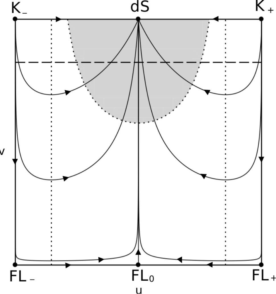
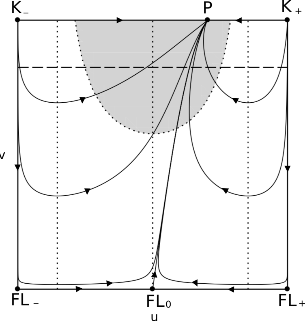
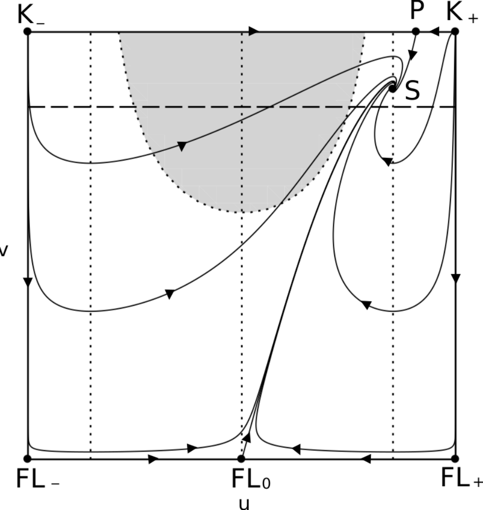
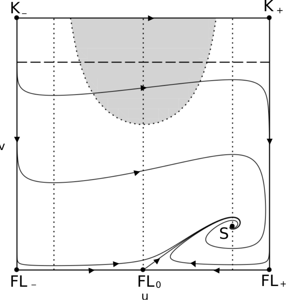
Finally, note that the fixed point in the state space at is replaced by the boundary set in the formulation, which consists of three fixed points, and , connected by the heteroclinic orbits . Since are saddles on the boundary, the two different formulations yield the same interior orbit structure, cf. Figure 3 in [21]. The different fixed points in the box state space for the variable in cases (i) and (ii) and their values for , and are summarized in Table 1.
| Name | ||||
3.3 Model classification and asymptotics
Recall that (apart from ) we for simplicity consider two cases: (i) a monotonically decreasing potential with ; (ii) a potential with a single positive minimum at such that , and , . Further subclassification is based on the combinatorial possibilities of the three parameter intervals (30) for and . As follows from the monotonic function given by (25), local analysis of the fixed points, and the complete description of the boundary orbit structures,1919 19 The asymptotics for the orbits on the boundaries were given in connection with the constant models while the asymptotics for the orbits on the boundary are quite straightforward as well. this yield the different asymptotic possibilities and global orbit structures for (i) and (ii) (in case (ii) is the future attractor for all interior orbits, and also for the orbits on the scalar field dominated boundary ).
We will now describe the asymptotics for the interior orbits, i.e. orbits for which , , , thereby describing solutions with and , for the two cases (i) and (ii):
- (i)
Except for a one-parameter set of heteroclinic orbits originating from , where one orbit originates from each fixed point, a one-parameter set of heteroclinic orbits from when , and one heteroclinic orbit from when , all interior orbits originate from the source , and also from when .
- (ii)
Except for a one-parameter set of heteroclinic orbits originating from , where one orbit originates from each fixed point, a one-parameter set of heteroclinic orbits from () when (), and one heteroclinic orbit from () when (when ), interior orbits originate from the heteroclinic cycle if and ,2020 20 More precisely, the heteroclinic cycle is their so-called -limit set. A heteroclinic cycle is a closed heteroclinic chain, where the latter consists of a concatenation of heteroclinic orbits, where the ending fixed point of one heteroclinic orbit is the starting fixed point of the next one. and otherwise from , which is a source when , or/and from , which is a source when .
Let us now for simplicity restrict the monotonic case (i) to , since this yields future eternal acceleration. Then the future asymptotics for the interior orbits for (i) and (ii) are as follows:
- (i)
All interior orbits end at the future attractor () when ().
- (ii)
All interior orbits end at the future attractor .
As a consequence of the above, all interior orbits are heteroclinic orbits, as are all boundary orbits apart from the fixed points, except in the case (ii) when and , since the past attractor, , then is the above mentioned heteroclinic cycle. All the above statements can be formally proved by using the monotonic function in (25), the completely known structure of the boundary sets, notably the global results in [21], and the local analysis of the fixed points, but for brevity we refrain from doing so here.
The above asymptotic properties lead to a useful result concerning . All interior orbits are future asymptotic to fixed points that satisfy and they are all, except for the one-parameter set of unstable manifold orbits of and the single unstable manifold orbits of and , past asymptotic to a fixed point at , or the heteroclinic cycle at , i.e. they originate from . Any generic interior orbit hence attains a positive minimum value of , and thereby , referred to as , at some intermediate time, where it follows from (18b) that this minimum occurs when , i.e. when .
4 Overview of bounded quintessence
In this section we give an overview and classification of various types of quintessence using the present state space formulation. We also give some of the key formulas for comparisons between the CDM model and quintessence models, noting that due to the observational success of the CDM model, viable quintessence models presumably cannot deviate too much from CDM.
4.1 The CDM model
The CDM model has the following key characteristics:
| (31a) | ||||
| (31b) | ||||
| (31c) | ||||
where the expressions for and the Hubble variable follow from spatial flatness, , , and energy conservation (also, recall that ). Setting , it follows from (31c) that at . We therefore expect that viable quintessence models begin accelerating when , (see Figure 3).2121 21 Recall that the redshift is defined as and hence that .
The basic criterion for quintessence evolution is that there is an early stage in the universe in which the matter dominates the scalar field, , , followed by a decrease (increase) in () to its present day value of approximately . To obtain a sense of at what time matter domination starts to decline and begins to effect the evolution of the universe we can use equation (31a) to show that
| (32) |
when , i.e. the effect of is felt only during the last few -fold(s) before the present time. The matter (dust) dominated epoch is preceded by a radiation epoch. Since , where thereby when (the redshift at decoupling corresponds to ), which together with that matter domination ends at indicates that the matter (dust) dominated epoch is long. We expect similar results for observationally viable quintessence models.
4.2 Quintessence relations
A similar calculation as for the CDM model results in the following quintessence relations:
| (33a) | ||||
| (33b) | ||||
| (33c) | ||||
Equation (33a) shows that (and thereby since ) determines , which in turn yields and .
Quintessence evolution is defined to begin during matter dominance when , and hence . The scalar field is then effectively a test field that does not affect the evolution of spacetime, as can be seen from (33b), which yields
| (34) |
During matter dominance, for not too large , is driven toward () since , but this behaviour has no observable significance. After the early matter dominated epoch a quintessence model should, like the CDM model, have a monotonic increase of , which requires , until , where, eventually, , since at the future global sink .
Basset et al. (2008) [23] state that nucleosynthesis yields the bound , which also holds during decoupling in the matter dominated epoch. We therefore divide evolution relevant for quintessence as follows:
- •
a matter dominated epoch during which
(35) and hence , where the scalar field is approximately a test field, and
- •
a quintessence epoch where and while . This epoch is subdivided into an observable quintessence epoch from when to the present where , and a future quintessence epoch when evolves from to .2222 22 The details of the bounds for (significant) quintessence (content) evolution will change as observations become increasingly accurate. This, however, will not affect our qualitative conclusions, which are robust under such changes.
At the end of section 3.3 we showed that on a generic interior orbit the variable attains a positive minimum value at some intermediate time. Thus a necessary condition for a generic interior orbit to have a matter dominated epoch with is that .
Since the quintessence evolution of and for observationally viable quintessence models presumably differs by less than when compared to CDM, equation (32) suggests that the observational quintessence epoch takes place between () and . Furthermore, as discussed earlier, the quintessence epoch is preceded by a matter (dust) dominated epoch with . Moreover, combining the matter dominated epoch with a preceding radiation dominated epoch, here neglected, leads to . From a dynamical systems perspective radiation and dust structurally are quite similar and we will therefore for simplicity in this paper replace radiation with dust and assume that during the matter dominated epoch (the role of inflation preceding the radiation dominated epoch will be dealt with in a future paper [20]). Such a long matter dominated -fold interval severely restricts viable initial data and is only possible for orbits that come extremely close to one or several of the fixed points , or (when ).
4.3 CDM and quintessence comparisons
In the introduction we noted that the CDM model can be thought of as a special quintessence model with constant potential and constant scalar field and equation of state parameter . In order to compare a quintessence model with the CDM model we identify the models at the present time as regards rate of expansion and matter content. Specifically we require that
| (36) |
where and are the observed Hubble parameter and the dimensionless Hubble-normalized matter density at the present time.
From (31) and (33) it follows that
| (37a) | ||||
| (37b) | ||||
which leads to the inequalities
| (38a) | ||||||||
| (38b) | ||||||||
where the inequalities for the Hubble variable also follow from
| (39) |
For the present models, which comprise the two cases (i) and (ii), introduced earlier following eq. (27), there are several different types of quintessence, which we now characterize, beginning with (i).
4.4 Monotonic potentials
In this subsection we consider models with a monotonically decreasing potential (case (i)) with . We first note that for interior orbits (as well as for interior orbits on the , boundary)
| (40) |
as follows from (21b). Hence acts as a semi-permeable membrane for the dynamics, which together with the monotonic function and local fixed point analysis implies that orbits with initial data eventually enters the invariant part of the state space. This corresponds to that a scalar field that is initially moving toward the potential ‘wall’ eventually bounce against it (recall that due to eq. (20)).
Thawing and freezing quintessence
Caldwell and Linder (2005) [15] defined thawing as when and freezing as when . This motivates defining a thawing quintessence model as a model for which and at the beginning of the observational quintessence epoch, which commences when at some -fold time . In analogy, a freezing quintessence model is characterized by and at . Note that the thawing (freezing) property may change sometime later during the quintessence epoch.
Thawing and freezing quintessence models correspond to orbits that are schematically described as follows:
- (U)
a one parameter family of heteroclinic ‘U-orbits’ , i.e. the unstable manifolds of the fixed points of that join a fixed point with to the future attractor (the fixed point when ; when ), where U stands for ‘unstable’.
- (S)
an open set of ‘S-orbits’
(41)
that shadow the U-orbits during intermediate and late times, where S stands for ‘shadowing’. The past attractor depends on , which complicates the details of the first step. When (for which ) the first step is or ; when (for which ) the first case still holds, but the second is replaced by the sequence .2323 23 Which of the two routes, and that is taken can be understood heuristically. The first case corresponds to that there is sufficient early matter content to create enough early matter dominated friction so that the scalar field (almost) freezes to a constant value before a ‘soft’/slow scalar field bounce in the matter dominated regime; the second case corresponds to that there is sufficient kinetic scalar field content to produce a ‘sharp’/fast scalar field bounce during an early scalar field dominated stage, i.e., the route is determined by the past ratio between the (kinetic) scalar field energy density and the matter energy density (obtainable from the linearization at ).
The number of -folds spent by S-orbits during the matter-dominated epoch, where , and hence , is highly dependent on the minimum value of at ; the smaller the more -folds, since this implies that S-orbits come closer and thereby stay longer near the fixed points. As discussed, viable models must spend -folds during the matter dominated epoch. This forces to be very small, and hence an S-orbit will intermediately shadow or very closely. This is subsequently followed by shadowing of the U-orbit , where shadowing is further strengthened by the fact that all interior orbits end at the future attractor . As a consequence the U-orbits describe the quintessence epoch of the S-orbits extremely well. Before shadowing , with frozen , the S-orbits shadow orbits on the boundaries (the stable manifolds of the fixed points , see Figure 1(c)) very closely, since the small value of results in coming very close to .
We can draw some general conclusions about the models that are described by the S-orbits. Recall that, before the quintessence epoch, S-orbits shadow orbits on the boundaries , where , followed by shadowing of , where at . Hence the quintessence epoch for S-orbits is characterized by a preceding stage where is approximated by a step function that steps down from to ; the time of the rapid drop in is determined by how closely is shadowed (i.e. it is determined by ), illustrated by the discussion in connection with Figure 4(c) in the next section.
The distinction between thawing and freezing quintessence models is due to the behaviour of along the U-orbits . We first consider the case so that . Then at both endpoints of the U-orbits, which implies that along each orbit must attain at least one local maximum (colloquially, a ‘bump’), where changes sign from positive (thawing) to negative (freezing). The details depend on the value of . Loosely speaking, for small , i.e. , there is a single bump of small amplitude occurring after the beginning of the quintessence epoch at , leading to a thawing quintessence model ( at ), illustrated by Figures 4(c) and 5(b), with , in the next section. As increases the amplitude of the bump increases and it occurs earlier, eventually before , leading to a freezing quintessence model ( at ), illustrated by in Figure 5(b) in the next section. Further increase of eventually leads to scaling freezing quintessence (see below).
In the case is replaced with , where , which leads to a plateau in the graph of as for each U-orbit. When this leads to greater variability in the graph in the observational quintessence epoch, e.g. for some values of a bump does not occur, as exemplified in Figure 6(b) below.
Scaling freezing quintessence
Scaling freezing quintessence occurs for monotonically decreasing potentials (i) with and is characterized by an approximate scaling behaviour initially, i.e. and and hence , for at least some -folds in the matter dominated regime () followed by freezing into the quintessence epoch. Scaling freezing quintessence models are associated with the unstable manifold of the scaling fixed point , which we recall is given by with , . Since the (freezing) quintessence epoch must be preceded by a matter dominated scaling epoch it follows that the fixed point must be located in the matter dominated region of state space (, see (35)), which requires .
Scaling freezing quintessence models are described by orbits of the following types:
- (U)
a single heteroclinic scaling freezing orbit (the unstable manifold of ) that joins the scaling fixed point to the future attractor (the fixed point when ; when ),
- (S)
an open set of heteroclinic shadowing orbits that come very close to during an intermediate stage of their evolution and afterward shadow the scaling freezing orbit :
(42)
where the separate stages are illustrated in Figures 5(a) and 6(a).2424 24 There are similarities and differences between scaling orbit attraction and the attractor solution/orbit in inflationary cosmology. In both cases there is a stable manifold of co-dimension one of an isolated fixed point and a one-dimensional unstable manifold, the ‘attractor’ orbit. However, in contrast to the scaling orbit, which corresponds to a positive eigenvalue, the inflationary attractor solution corresponds to a zero eigenvalue and is thereby a center manifold orbit. The zero eigenvalue leads to that (A) the inflationary attractor orbit attracts nearby orbits much more strongly than the scaling orbit, (B) orbits stay much longer close to the de Sitter fixed point in a quasi-de Sitter stage than orbits stay close to . The refers to one of the orbits in the boundary set joining to , as shown in Figure 2(d). We note that is the source and is the sink for orbits in this boundary set, which facilitates the shadowing by the orbits (S). It is important to note that to obtain orbits for which the scaling property holds for several -folds in the matter dominated regime we have to ensure that the orbits (S) come extremely close to the scaling fixed point . We will achieve this in the numerical simulations in sections 5.2 and 5.3 by choosing appropriate initial values.
4.5 Scaling oscillatory and oscillatory quintessence
We now consider case (ii), i.e. a potential with a single positive minimum at that gives rise to the de Sitter fixed point as the future attractor. The unstable manifold of , which is the straight line , terminating at (i.e. the heteroclinic orbit ), corresponds to the CDM model. For brevity we consider the case when so that is an attracting spiral, which causes orbits to spiral around the straight CDM orbit as they approach . Hence for non-CDM orbits oscillates around and oscillates around while increases to as , which implies that undergoes continuing oscillations with damped amplitude as the future attractor is approached. Thus, in the observable quintessence epoch there are a finite number of oscillations of with changes in the sign of , i.e. the evolution successively changes between thawing and freezing.
There are numerous pre-quintessence possibilities, depending on the values of and . As an example we will consider and , which means that the scaling fixed points and come into play. The unstable manifolds of spiral around the straight line orbit as they approach . We divide quintessence orbits for models with and into two classes:
- •
Scaling oscillatory quintessence is described by the scaling orbits and , and orbits that come extremely close to or . These latter orbits subsequently shadow the scaling orbits and exhibit the scaling property during part of the matter dominated epoch, followed by oscillations in the quintessence epoch.
- •
Oscillatory quintessence is described by orbits, and orbits that shadow these orbits, not coming extremely close to or , thereby not exhibiting the scaling property during part of the matter dominated epoch, but they still undergo oscillations in the quintessence epoch.
For examples, see Figure 7(a); note, however, that generic orbits originate from , which for these models is the heteroclinic cycle on the boundary of the boundary.
5 Example: The double-exponential potential
In this section we will illustrate some aspects of the previous general discussion about quintessence using special cases of a simple example: the double-exponential potential,
| (43) |
We will represent the orbits using figures in the box state space, augmented with graphs of and .2525 25 The double-exponential potential models have a fairly lengthy history in the literature. An early paper is Barreiro et al. (2000) [24]; see also, e.g., Barro Calvo and Maroto (2006) [25], section IIB, Bassett et al. (2008) [23], section 3.2 and Dunega et al. (2013) [26], eq. (A.3). In particular [23] have given simulations of for initial data that in effect yields the scaling orbit using and several positive values of between and , as well as negative values between and , see their Figure 2, lower left panel; note that the temporal range they use is , which corresponds to . To include the potential (43) in the present framework we introduce the bounded variable
| (44) |
It follows that is a linear function of given by
| (45) |
Before beginning, for the purpose of comparison, we represent the CDM model by orbits in the box state space. We have noted that the CDM model can be viewed as a limiting quintessence model with constant potential and a constant scalar field, which results in (). Since it follows from (21b) that the set is an invariant set and that the orbits that represent the CDM model are straight lines . Figure 4(a) shows this one-parameter set of CDM orbits which join the fixed points to the de Sitter fixed points . We will see that the invariant set in the constant potential case, and the CDM orbits that it contains, becomes deformed for varying potentials.
We will use the following four illustrative choices of the parameters :
- 1)
the monotonic potential with , ;
- 2)
the monotonic potential with , ;
- 3)
the monotonic potential with , ;
- 4)
a potential with a positive minimum for which , with , being a stable spiral since , where , since (45) results in
(46)
5.1 Case 1: ,
This case illustrates the box state space for the double exponential potential, augmenting Figure 1(c) with information that depends on the values of , namely the fixed points and and the stability of the kinaton fixed points indicated by the arrows on the orbits joining them. The details of the orbits in the boundary sets are given in Figures 2(a) and 2(b), respectively. Figure 1(c) also shows the orbits in the boundary sets and in the base of the box .


Figure 4(b) depicts the unstable manifold with , and two orbits that shadow this orbit during its (thawing) quintessence epoch. The two shadowing orbits, which link the past attractor to the future attractor, are schematically described by the sequence2626 26 See the earlier discussion in connection with (41).
| (47) |
Figure 4(c) illustrates the ‘bump’ that appears in the graph of for all three orbits, where the maximum of the bump occurs after . Thus all three orbits describe thawing quintessence models. The graphs for the shadowing orbits show the step function behaviour of from to that arises from the transition , described in section 4.4.
Figures 4(b) and 4(c) show that the two shadowing orbits have an epoch of matter domination of relatively short duration . This duration is determined by the minimum value of or equivalently of , which for the two shadowing orbits is given by . In order to obtain a model with a more realistic value of we have to use shadowing orbits with at . This yields orbits that shadow the quintessence -orbit originating from so closely so that they are indistinguishable from it during the quintessence epoch; moreover, before the matter dominated stage these orbits shadow the orbits with on the subsets, illustrated in Figure 1(c), extremely closely. This exemplifies the strong restrictions a long matter dominated epoch imposes on initial data.
5.2 Case 2: ,
This case illustrates thawing, freezing and scaling freezing quintessence. Figure 5(a) depicts the scaling orbit and five -orbits. The orbit with initially shadows the orbit with very closely which brings it close enough to so that it has an approximate (matter dominated) scaling property when (to have longer period of scaling, e.g. , requires orbits to be even closer to , and hence to ); this is followed by shadowing of the scaling orbit and hence is an example, as is the scaling orbit, of scaling freezing quintessence, in accordance with section 4.4.
The remaining other orbits in Figure 5(a) illustrate the transition from thawing to freezing quintessence as and thereby varies, as shown by the graphs of in Figure 5(b). We see that the -orbits exhibit a ‘bump’ in with a maximum that increases and moves to more negative as increases: the -orbits with describe thawing quintessence while orbits with larger values of , but not too large since they then yield scaling freezing quintessence, describe freezing quintessence. There are also two open sets of thawing and freezing quintessence orbits (not shown in the figure) that shadow these -orbits during the quintessence epoch. Before this quintessence epoch they either shadow orbits on the boundary and then make the transition or they shadow the heteroclinic sequence and then orbits on the boundary followed by the transition . These models thus exhibit a step like behaviour in between and before the quintessence epoch, as in case 1.
Finally, Figure 5(c) shows the graph for the depicted orbits in the state space. The Hubble variable deviates from with less than during the quintessence epoch.


5.3 Case 3: ,
This case illustrates the effect on the quintessence epoch of replacing with a value in the range , which changes the future attractor from to . A change from to has negligible observational effects, but if then is non-negligible, so that increasing increasingly affects the observational quintessence epoch that begins at and ends at . This is illustrated by the orbits and associated graphs in Figure 6. Figure 6(b) shows that for sufficiently small and sufficiently large the ‘bump’ in is replaced by continued thawing followed by a plateau, while for larger the continued freezing is replaced with a minimum in where subsequent thawing is levelled out to the asymptotically future plateau. This increases the deviation of from during the observational quintessence epoch so that future observations will impose increasingly restrictive bounds on .


5.4 Case 4: ,
This case illustrates the effect on the quintessence epoch by replacing with . Figure 7(a) shows the scaling orbits originating from and and some -orbits. The scaling orbits are asymptotic to the fixed point and spiral around the straight line CDM orbit as they approach . The scaling orbits describe models with a scaling phase in part of the matter dominated epoch followed by oscillations of . For this reason we referred to this type of models as scaling oscillatory quintessence models, in section 4.5. The orbits that originate from with extremely close to (respectively ) shadow the scaling orbit from (respectively ) and hence also describe scaling oscillatory quintessence (as does other, non-illustrated, open sets of orbits that shadow orbits on the boundaries and come extremely close to ). In contrast, the orbits -orbits in 7(a) with that are not extremely close to do not have a scaling phase and are examples of models that we referred to as oscillatory quintessence models in section 4.5.
Figures 7(b) and 7(c) show the graphs of and for values of . Figure 7(b) shows the familiar steep drop in from the plateaux at that characterizes scaling oscillatory quintessence.2727 27 Increasing moves the steep drop in for the scaling (freezing) orbit (scaling (oscillatory) orbit) in Figure 5(b) (Figure 7(b)) to increasingly negative , in agreement with Figures 5 and 9 in Bag et al. (2018) [27]. Figure 7(c) shows that deviates from very little during the quintessence epoch, for both scaling oscillatory quintessence and oscillatory quintessence. When compared with Figure 5(c)2828 28 For example, the graph in Figure 7(c) with has , while the graph in Figure 5(c) with has . this suggests that potentials with a positive minimum and yield quintessence evolution that is closer to CDM evolution than monotonic potentials for which .


6 Concluding remarks
In this paper we have analyzed different types of quintessence that arise for scalar field potentials for which is bounded with limits , using a new regular dynamical system on a three-dimensional bounded ‘box state space’ , illustrated with specific double exponential potential examples. The box state space made it possible to systematically explore the entire solution space of models with bounded . This new formulation also highlighted that quintessence dynamics is described by the one-dimensional unstable manifold orbits of the fixed points and . These orbits describe the dynamics during the quintessence epoch, when is increasing and beginning to influence the cosmological expansion. In order to model the matter-dominated epoch which precedes this epoch one has to consider an open set of orbits that originate at the past attractor and shadow the unstable manifolds during the quintessence epoch. The requirement of a sufficiently long matter dominated epoch (of order -folds) requires orbits to come very close to one or more of the fixed points , in the matter dominated part of the state space. This severely restricts viable quintessence initial data but has the advantage that the open set of orbits subsequently shadow the unstable manifold orbits very closely, which thereby describe quintessence.
Analysis of the unstable manifold orbits revealed a rather wide range of dynamical possibilities during the quintessence epoch. This resulted in an extension of the quintessence classification of Tsujikawa (2013) [14] for models with bounded from thawing quintessence and scaling freezing quintessence to also include freezing quintessence, scaling oscillatory quintessence and oscillatory quintessence, where the last two types occur for potentials with a sufficiently steep positive minimum (i.e. potentials with ).
More precisely, thawing quintessence evolution is described by rolling down a monotonic potential according to when , while freezing quintessence arises when is large, but avoiding a large (recall the general ‘bump’ discussion in section 4.4 exemplified and illustrated in sections 5.1, 5.2 and 5.3); scaling freezing quintessence evolution is described by rolling down a monotonic potential according to , see section 4.4 and sections 5.2 and 5.3 for illustrations (in all these cases when , when ). Scaling oscillatory quintessence and oscillatory quintessence evolution arise for potentials with a minimum where , where scaling oscillatory quintessence evolution is described by the scaling orbits and orbits that shadow them extremely closely, thereby allowing scaling in part of the matter dominated epoch, while oscillatory quintessence evolution corresponds to orbits and an open set of orbits shadowing these orbits, where is not too close to ; see section 4.5 for the general discussion and section 5.4 for examples and illustrations.
These various types of quintessence evolution were illustrated in section 5, but there are also some illustrative results in the literature:
- i)
Thawing quintessence: See Figures 4, 5 and 6 and also Akrami et al. (2020) [7], Figure 1, top (lower) panel, with ().2929 29 There are also examples in the literature where thawing quintessence corresponds to slowly rolling down a local monotonic part of a potential, e.g. the hilltop potential (which can be treated globally with the present formulation since is bounded, although we, for brevity, omit to do so), see Figure 2 in Yang et al. 2019 [28]. Another example is the PNGB potential , which describes thawing quintessence as long as the scalar field is slowly rolling down a potential slope (see, e.g., Tsujikawa (2013) [14] section 3.3). In this case, however, the time period for thawing is limited since the slow roll is interrupted by oscillations at the potential minimum. Due to that at the minimum, this potential is not globally covered by the present formulation, but the oscillatory evolution can be described by using a modification of the methods given by Alho et al. (2015) [29].
- ii)
- iii)
- iv)
Scaling oscillatory quintessence: See Figure 7; Barreiro et al. (2000) [24], Figure 3;3030 30 This paper shows on the same axes for two cases of the double exponential potential, , scaling freezing quintessence; , scaling oscillatory quintessence. Bassett et al. (2008) [23], figure 2; Bag et al. (2018) [27], Figure 5.
- v)
Oscillatory quintessence: See Figure 7; Yang et al. 2019 [28], Figure 1.3131 31 The graph of shows a drop from to (corresponding to initial data close to followed by shadowing ) and subsequent oscillations with an initial large ‘bump’ with an amplitude . There are no radiation or dust plateaus at and , respectively for and the model thereby have no radiation or dust scaling epochs.
In the present work we have for simplicity restricted matter to be dust, but in future work we will include radiation in an extended state space description, which have the present state space as an invariant dust boundary, and an analogous invariant radiation boundary where the dust content is zero. For large (and in the potential minimum case) this leads to two scaling plateaus for scaling freezing quintessence (and scaling oscillating quintessence): one for radiation at , corresponding to orbits originating from, or coming very closely to, a scaling fixed point on the radiation boundary, and one plateaux at , associated with that the radiation scaling orbit(s) come extremely close to the scaling fixed point at the dust boundary after the radiation-dust transition. This gives a dynamical systems description of these two plateaus in the graphs for scaling freezing and scaling oscillatory quintessence for the radiation and dust case in the literature, see Barreiro et al. (2000) [24], Figure 3, and Bag et al. (2018) [27], Figures 5 and 9.
As mentioned in the introduction, Tsujikawa (2013) [14], following Steinhardt et al (1999) [30], defined tracking freezing quintessence for potentials which satisfy , e.g. the inverse power law potential. 3232 32 Steinhardt et al. (1999) [30] introduced the term ‘tracking solutions’ to describe this form of quintessence (a wide range of initial conditions rapidly converge to a common evolutionary track). Tsujikawa added the qualifier ‘freezing’ since . For brevity we will use the name tracking quintessence. For such potentials the new dynamical system (21) is not regular, since appears on the right hand side of the equations. We have recently found an alternate set of variables that overcomes this difficulty, i.e. the resulting dynamical system is regular, but at the expense of a new variable that is unbounded. This alternate system has enabled us to describe tracking quintessence from a state space perspective in terms of the unstable manifold of a matter dominated ‘tracking’ fixed point, which we refer to as the ‘tracking orbit’, and an open set of nearby orbits that track, i.e. shadow, the tracking orbit.3333 33 There is an analogy with the scaling orbit and the representation of scaling freezing quintessence in the present paper. Although the state space is unbounded, the tracking orbit and the open set of shadowing orbits during matter domination and quintessence evolution, are confined to a bounded region of the state space. Our treatment of tracking quintessence will be given in a subsequent paper.
In yet another paper we will use the new ‘tracking dynamical system’ and the ‘tent state space’ formulation to derive new, simple, and accurate approximation formulas for key quantities such as and in a systematic and unified manner for the various types of quintessence, thereby complementing earlier work in the literature.3434 34 See, for example [14], section 3 for a review.
Acknowledgments
AA is supported by FCT/Portugal through CAMGSD, IST-ID, Projects No. UIDB/04459/2020 and No. UIDP/04459/2020. CU would like to thank the CAMGSD, Instituto Superior Técnico in Lisbon, Portugal, for kind hospitality.
References
- [1] A. G. Riess et al. Observational evidence from supernovae for an accelerating universe and a cosmological constant. Astron. J., 116:1009, 1998.
- [2] S. Perlmutter et al. Measurements of omega and lambda from 42 high redshift supernovae. Astron. J., 517:565, 1999.
- [3] N. Suzuki et al. The hubble space telescope cluster supernov survey. v. improving the dark-energy constraints above and building an early-type -hosted supernova sample. Astro. Phys. J., 746:85, 2012.
- [4] P.A.D Ade et al. Planck 2015 results xiv. dark energy and modified gravity. Astron. and Astrophys, 594:A14, 2016.
- [5] T. Chiba, A. De Felice, and S. Tsujikawa. Observational constraints on quintessence: Thawing, tracker and scaling models. Phys. Rev. D, 87:083505, 2013.
- [6] R. R. Caldwell, Rahul Dave, and Paul J. Steinhardt. Cosmological imprint of an energy component with general equation of state. Phys. Rev. Lett., 80:1582–1585, 1998.
- [7] Y. Akrami et al. Quintessential -attractor inflation: forecasts for stage iv galaxy surveys. JCAP, 04:006, 2021.
- [8] E. J. Copeland, A. R. Liddle, and D. Wands. Exponential potentials and cosmological scaling solutions. Phys. Rev. D, 57:4686, 1998.
- [9] C. B. Collins. More qualitative cosmology. Comm. Math. Phys., 23(2):137–158, 1971.
- [10] J. Wainwright and G. F. R. Ellis. Dynamical systems in cosmology. Cambridge University Press, 1997.
- [11] A. A. Coley. Dynamical systems and cosmology. Kluwer Academic Publishers, Dordrecht, 2003.
- [12] S. Bahamonde, C. G. Böhmer, S. Carloni, E. J. Copeland, Wei Fang, and N. Tamanini. Dynamical systems applied to cosmology: Dark energy and modified gravity. Physics Reports, 775-777:1–122, 2018.
- [13] A. Alho and C. Uggla. Scalar field deformations of lambda-cdm cosmology. Phys. Rev. D, 92(10):103502, 2015.
- [14] S. Tsujikawa. Quintessence: a review. Class. Quantum Grav., 30:214003, 2013.
- [15] R. R. Caldwell and E. V. Linder. Limits of quintessence. Phys. Rev. Lett., 95:141301, Sep 2005.
- [16] A. A. Coley, J. Ibánez, and R. J. van den Hoogen. Homogeneous scalar field cosmologies with an exponential potential. Journal of Mathematical Physics, 38:17, 1997.
- [17] L. A. Urena-Lopez. Unified description of the dynamics of quintessential scalar fields. JCAP, 2012:035, 2012.
- [18] W. Fang, Y. Li, K. Zhang, and H.-Q Lu. Exact analysis of scaling and dominant attractors beyond the exponential potential. Class. Quantum Grav., 26:155005, 2009.
- [19] A Nunes and J P Mimoso. On the potentials yielding cosmological scaling solutions. Physics Letters B, 488:423, 2000.
- [20] A. Alho and C. Uggla. Quintessential -attractor inflation: A dynamical systems analysis. Preprint, 2021.
- [21] A. Alho, W. C. Lim, and C. Uggla. Cosmological global dynamical systems analysis. Class. Quantum Grav., 39:145010, 2022.
- [22] Michael Joyce and Tomislav Prokopec. Turning around the sphaleron bound: Electroweak baryogenesis in an alternative post-inflationary cosmology. Phys. Rev. D, 57:6022–6049, 1998.
- [23] Bruce A Bassett et al. Is the dynamics of scaling dark energy detectable? J. of Cosmology and Astroparticle Physics, 07:007, 2008.
- [24] T Barreiro, E. J. Copeland, and N. J. Nunes. Quintessence arising from exponential potentials. Phys. Rev. D, 61:127301, 2000.
- [25] G. Barro Calvo and A. L. Maroto. Confronting quintessence models with recent high-redshift supernova data. Phys. Rev. D, 74:083519, 2006.
- [26] D. G. A. Duniya, D. Bertacca, and R. Maartens. Clustering of quintessence on horizon scales and its imprint on hi intensity mapping. J. of Cosmology and Astroparticle Physics, 10:015, 2013.
- [27] S. Bag, S.S. Mishra, and V. Sahni. New tracker models of dark energy. Journal of Cosmology and Astroparticle Physics, 08:009, 2018.
- [28] W. Yang, M. Shahalam, B. Pal, S. Pan, and A. Wang. Constraints on quintessence scalar field models using cosmological observations. Phys. Rev. D, 100:023522, 2019.
- [29] A. Alho, J. Hell, and C. Uggla. Global dynamics and asymptotics for monomial scalar field potentials and perfect fluids. Class. Quant. Grav., 32(14):145005, 2015.
- [30] P. J. Steinhardt, L. Wang, and I. Zlatev. Cosmological tracking solutions. Phys. Rev. D, 59:123504, 1999.