Provably Uncertainty-Guided Universal Domain Adaptation

Since some known samples may be distributed far away from the centers of the source classes, and unknown samples may be distributed in the edges of the source clusters due to the domain discrepancy, clustering target samples with their nearest neighbors or nearest prototypes is dangerous in the original feature space. Therefore, we propose to find a reliable linear subspace to deal with the above problems and improve the accuracy of discovering the unknown samples based on the neighborhood information searched from source domain. Specifically, given $Z^{s}=[\mathbf{z}^{s}_{0},\mathbf{z}^{s}_{1},\cdots,\mathbf{z}^{s}_{N_{s}}]^{\mathsf{T}}\in\mathbb{R}^{N_{s}\times m}$ and $\mathcal{B}=[\mathbf{z}^{t}_{0},\mathbf{z}^{t}_{1},\cdots,\mathbf{z}^{t}_{b}]^{\mathsf{T}}\in\mathbb{R}^{b\times m}$, where $m$ means the dimension of $\mathbf{z}_{i}$, $Z^{s}$ and $\mathcal{B}$ are sets of all source samples and target samples in a mini-batch respectively, we denote the original feature set $Z=[\mathbf{z}_{0}^{s},\mathbf{z}^{s}_{1},\cdots,\mathbf{z}^{s}_{N_{s}},\mathbf{z}^{t}_{0},\mathbf{z}^{t}_{1},\cdots,\mathbf{z}^{t}_{b}]\in\mathbb{R}^{n\times m}$ where $n=N_{s}+b$.

Then, we have

where $P$ is a transformation matrix mapping the features with $m$ dimensions to reduced features with $p$ dimensions.

To get the $Z_{sub}$, we propose to analyze the covariance matrix of $Z$. After centralizing $Z$, the covariance matrix $A$ can be defined as:

Inspired by Wang et al. [53], the covariance matrix captures the feature distribution of the training data, and contains rich information of potential semantic differences. We propose to decompose the covariance matrix $A$ to find the dimensions which can best represent the semantic difference of each source class and cut off the other dimensions. After the reduction of dimensions, since the unknown target samples do not share the common features with the known source classes, the distances from an unknown sample to each of the source classes can be averaged which can lower $k_{max}$ in Eq. (1). Specifically, we leverage the singular value decomposition (SVD) method to decompose the covariance matrix $A$:

Then, we can get the transformation matrix $P$ from $V$:

By projecting the original features to the linear subspace, we propose to search for the neighbors of each of the target samples in the subspace. Particularly, we firstly employ a memory bank $M$ to store all the features of the source samples:

with a momentum scheme to update the memory bank:

Then, we project the set $Z=[\textbf{m}_{0},\dots,\textbf{m}_{N_{s}},\mathbf{z}^{t}_{0},\mathbf{z}^{t}_{1},\cdots,\mathbf{z}^{t}_{b}]$ to $Z_{sub}$. We search for the neighbors $\mathcal{N}$ for each target sample $\mathbf{z}_{i}$ in $Z_{sub}$ and propose an uncertainty score of $\mathbf{z}_{i}$ according to Eq.(10):

where $k$ is the number of searched neighbors. Then, the discovered unknown samples are denoted as:

where $\tau$ is set manually. Similarly, the known samples are denoted as:

and $\mathbf{z}_{i}\in\hat{Z}^{k}$ has pseudo label $\hat{y}_{i}$ which is defined as:

As mentioned in the second condition of Corollary 4, the target sample should be close enough to its neighbors. However, ‘nearest’ neighbors is not equivalent to ‘most compact’ neighbors. For instance, for an unknown sample, which is far away from all source classes, its ‘nearest’ neighbors can also mostly belong to the same class which means that there are some noisy data in $\hat{Z}^{k}$. Moreover, since known ones might also distribute on the edges of clusters of the source classes, the distance from a centroid of a source class to a known sample might not be significantly different from the distance between the centroid and an unknown sample. Thus, it is hard to filter noisy known samples from $\hat{Z}^{k}$ through the $k$-nearest neighbor distance. Therefore we introduce a dynamical $\delta$-filter scheme to remove the noisy data.

To be specific, as shown in Fig. 4, compared to the compactness of the class $\hat{y}_{i}$, a credible known sample $\mathbf{z}_{i}\in\hat{Z}^{k}$ with its neighbors belonging to class $\hat{y}_{i}$ should be compact enough. To estimate the compactness of $\mathbf{z}_{i}$ and its neighbors, we apply the spectral decomposition on the covariance matrices of these vectors ( i.e., $\mathbf{z}_{i}$ and its neighbors belonging to class $\hat{y}_{i}$) to get the maximum eigenvalues of the covariance matrices which can represent the dispersion of the vectors. Moreover, to get a comparable estimation of the dispersion of vectors in class $\hat{y}_{i}$, we randomly select a sample from the source class $\hat{y}_{i}$ which is not a neighbor of $\mathbf{z}_{i}$ and compute the maximum eigenvalue of the covariance matrix of the selected vector and the neighbors belonging to class $\hat{y}_{i}$. We leverage the difference of the two eigenvalues to determine whether $\mathbf{z}_{i}$ is noisy.

In detail, for $\mathbf{z}_{i}\in\hat{Z}^{k}$, we denote $\mathcal{N}^{\prime}_{i}=\{h_{0},h_{1},\dots,h_{n^{\prime}}\}$ as the neighbors of $\mathbf{z}_{i}$ where samples in $\mathcal{N}^{\prime}_{i}$ belong to class $\hat{y}_{i}$ and $n^{\prime}=|\mathcal{N}^{\prime}_{i}|>\tau$. Next, we can denote two zero-mean matrices defined as:

where $h_{n^{\prime}+1}$ means the selected source sample. Then, we can get the covariance matrices of both sets:

We leverage spectral decomposition on both covariance matrices to get maximum eigenvalues $\lambda_{i}$ and $\hat{\lambda}_{i}$ of $\Sigma_{i}$ and $\hat{\Sigma}_{i}$ respectively. Finally, we define the difference value $\delta_{i}$ as:

When $\delta_{i}$ is bigger, it means that including $\mathbf{z}_{i}$ has a significantly bad influence on the description of the vector set and $\mathbf{z}_{i}$ should be filtered out from $\hat{Z}^{k}$. Experimentally, we assume that a clean known target sample should satisfy $\delta_{i}\leq 0.2\lambda_{i}$.

Using the traditional CE-loss training on the source domain usually leads to a problem of imbalance between the predictions of the known/unknown target samples. Learning on source classes $Y^{s}$ is much faster than that on the unknown class $Y^{unk}$ due to the supervised objective which leads the whole model to be biased towards the common classes $Y^{com}$ in the target domain. As a result, the intra-class variance of the source domain can be much smaller than that of the target domain, including known target classes and the unknown class. The biased model can cause the overconfident predictions for many unknown samples. Therefore, it is important to balance the intra-class variances of both domains. We propose a new uncertainty-guided margin loss (UGM) to achieve that. Specifically, at the beginning of the training, we enforce a larger margin to encourage a larger intra-class variance which is similar to the intra-class variance of discovered unknown samples. The margin $\mu$ goes down to zero close to the end of the training,

where the margin $\mu$ represents the intra-class variance of $\hat{Z}^{unk}$ which is defined as:

where $\mid\cdot\mid$ means the number of elements in a set. We normalize the weights and inputs, i.e., $W_{y_{i}}^{\mathsf{T}}=\frac{W_{y_{i}}^{\mathsf{T}}}{|W_{y_{i}}^{\mathsf{T}}|}$ and $\mathbf{z}_{i}=\frac{\mathbf{z}_{i}}{|\mathbf{z}_{i}|}$.

Since we use the entropy of the classifier output to distinguish the unknown samples, we need to lower the confidence of unknown samples belonging to $\hat{Z}^{unk}$. We employ the $\mathcal{L}_{unk}$ to smooth the posterior distribution for unknown inputs to increase the entropy:

where the inputs of Eq. (32) belong to the discovered unknown samples set $\hat{Z}^{unk}$.

Moreover, to reduce the influence of the domain misalignment, it is necessary to make each source class more compact and discriminative to enlarge the gap between two source classes which can improve the consistency of neighbors’ labels for a known target sample when it searches the nearest neighbors from the source domain. Thus, we employ a supervised contrastive learning loss [36] $\mathcal{L}_{sup}$ to make data points in the source domain more compact by pushing the samples from different classes apart while pulling the samples from the same class closer. $\mathcal{L}_{sup}$ is given by:

where $\mathcal{A}^{+}_{i}$ and $\mathcal{A}^{-}_{i}$ represent the positive samples in $M$ with the same label as $\mathbf{z}_{i}$ and the negative samples searched from $M$, respectively. $t$ is a temperature parameter.

The total training loss of our method can be computed as

where $\lambda$ is a weighting parameter. Moreover, the full algorithm of our method is provided in Algorithm 1.

We conduct experiments on four datasets. Office-31 [56] consists of $4,652$ images from three domains: DSLR (D), Amazon (A), and Webcam (W). OfficeHome [57] is a more challenging dataset, which consists of $15,500$ images from $65$ categories. It is made up of $4$ domains: Artistic images (A), Clip-Art images (C), Product images (P), and Real-World images (R). VisDA [58] is a large-scale dataset, where the source domain contains $15,000$ synthetic images and the target domain consists of $5,000$ images from the real world.

In this paper, we use the H-score in line with recent UniDA methods [17, 16, 5]. H-score, proposed by Fu et al. [17], is the harmonic mean of the accuracy on the common classes $a_{com}$ and the accuracy on the unknown class $a_{unk}$:

We employ the ResNet-50 [59] backbone pre-trained on ImageNet[60], and optimize the model using Nesterov momentum SGD with momentum of $0.9$ and weight decay of $5\times 10^{-4}$ . The batch size is set to $36$ through all datasets for both domains. The initial learning rate is set as $0.01$ for the classifier layers and $0.001$ for the backbone layers. The learning rate is decayed with the inverse learning rate decay scheduling. The number of neighbors retrieved is set to be dependent on the sizes of the datasets. For Office-31 ($4,652$ images in $31$ categories) and OfficeHome ($15,500$ images in $65$ categories), the number of retrieved neighbors $|\mathcal{N}_{i}|$ is set to $10$. For VisDA ($20,000$ images in total), we set $|\mathcal{N}_{i}|$ to $100$ , respectively. We set $\lambda$ to $0.1$ and $t$ to $0.05$ which are constant through all the datasets. In the test phase, the threshold of distinguishing the unknown samples is set to $\frac{\log C}{2}$ following DANCE [20] which used the entropy of the classifier’s output to determine the unknown samples.

We aim to show that our method can better balance the confidences of known and unknown samples for UniDA by comparing our method with the current SOTA methods, such as UAN [27] and DANCE [20], which employed a softmax-based classifier to produce the confidence of each sample to determine whether it belongs to the unknown class or not. Also, we compare our method with DANCE [20], DCC [5] and GATE [21] to show that it is better able to solve the domain misalignment by projecting features into a linear subspace rather than operating in the original feature space.

TABLE I lists the results on Office-31 with the OPDA and ODA settings respectively. TABLE II lists the results on OfficeHome and VisDA both with the OPDA and ODA settings, respectively. On Office-31, our method outperforms the SOTA methods by $1.2\%$ in terms of the H-score on average with the OPDA setting, and makes a significant improvement of $2.0\%$ in terms of the H-score on average with the ODA setting. For the more challenging dataset OfficeHome which contains much more private classes than common classes, our method also makes a significant improvement of $5.3\%$ in terms of the H-score with the ODA setting. Our method consistently performs better than other methods. VisDA is a much larger dataset than Office-31 and OfficeHome which contains about $10,000$ images in each domain. Our method achieves the SOTA performance on VisDA with the significant improvement of $3.7\%$ in the ODA setting.

According to the results of the quantitative comparisons, our method achieves the SOTA performance in every dataset and most subtasks, which demonstrates the effectiveness of the main idea of our method that solves the domain misalignment through mapping features into a linear subspace and balances the confidences of known and unknown samples by controlling the intra-class variance of the source domain.

By Corollary 4, the posterior probability of a target sample belonging to the unknown class depends on the largest number of neighbors belonging to the same class. Thus, we compare the proposed unknown samples discovering scheme with the discovering method based on the $k$-nearest neighbor distance in this part. Firstly, we collect the $k$-nearest neighbor distances of all target samples in an early epoch in Office-$31$ which can be more influential for the whole training. As shown in the first row in Fig. 5, the distributions of known samples are not distinguishable enough, especially in a$2$w, d$2$a and w$2$a. It is obvious that the $k$-nearest neighbor distance is not reliable enough to discover the unknown samples. Moreover, the optimal thresholds for each subtask is different and hard to choose. Notably, mapping samples into the linear subspace has a significant influence in making the distribution of data points more uniform as shown in the second row in Fig. 5. However, it is unable to improve the discrimination of unknown samples based on the $k$-nearest neighbor distance. By contrast, the distributions of confidences defined by the largest number of neighbors belonging to the same class illustrated in the first row of Fig. 6 are much more distinguishable.

Original feature space vs Linear subspace. The purpose of extracting a linear subspace is to make the distribution of data points more uniform so as to avoid the influence of the domain misalignment. Comparing the charts in the first row and the second row in Fig. 5, it is obvious that the data points in the subspace are similar in the distribution of the $k$-nearest neighbor distances. In Fig. 6, we conduct experiments on Office-$31$ to compare the distributions of the confidences produced by the proposed unknown samples discovering method in the original feature space (First row) and the linear subspace (Second row). Apparently, the distributions of confidences in the subspace are much more distinguishable than that in the original feature space. The overlaps between unknown and known samples are much fewer in the subspace which is benefited by reducing the misalignment between target samples and source samples.

Accuracy of the uncertainty estimation. We also conduct experiments on the accuracy of the uncertainty estimation on the original feature space and the subspace in some subtasks of Office-$31$ and OfficeHome where we plot the histograms of the accuracy of the uncertainty estimation in Fig. 7. The unknown samples are consistently detected with high accuracy which on average far surpasses $80\%$ and the performance of accuracy of unknown samples discovering method based on the uncertainty estimation in the subspace is much better than that in the original feature space. Thus, through the proposed unknown samples discovering scheme, our approach reliably finds the unknown samples in the target domain.

Quantitative comparison with different methods. To show the improvement on the distribution of the entropy which is used to classify the unknown samples in the test stage, we conducted experiments on Office-31 (a2d). First, we plot the distributions of the entropies of all samples in the target domain at the final epoch in Fig. 8(a). Then, we compare the plot to that trained on the source domain only in Fig. 8(b). We can observe that the full version of our method better distinguishes the known samples from the unknown ones. Furthermore, in Fig. 8(c), we show the corresponding plot produced by DANCE [20] for comparison. Noticeably, our method performs better than DANCE [20] in terms of distinguishing the known samples from the unknown ones.

Uncertainty-guided margin loss vs CE-loss. To show the effect of the uncertainty-guided margin loss on balancing the predictions of known and unknown samples, we track the entropy level of the unknown samples and the confidence level of known samples following the training process on Office-$31$. We recorded the mean value of entropies of predictions for unknown samples and the mean value of maximum prediction confidences output by the classifier of each known sample in every step. For comparison, we first plot records where the classifier was only trained on source domain with a traditional CE-loss like Eq. (29) in the first row of Fig. 9. We can observe that although the known samples consistently have high confidence, most of the unknown samples are significantly overconfident during the training process. In the second row of Fig. 6, we plot the records using the CE-loss and the proposed unknown loss as Eq. (32). The entropy level has been improved but the overconfidence of the unknown samples is still obvious. In the third row of Fig. 9, we plot the records using the proposed uncertainty-guided loss which can perfectly distinguish the unknown samples using entropy while retaining the known samples with highly confident predictions. We also employ t-SNE [61] pictures to visualize the distributions of target samples on Office-$31$ (A$2$D) in Fig. 10. We observe that the distribution of data points in ours (right) is much more discriminative than that of DANCE [20] (mid) and the model trained with the source dataset only (left).

Setting of uncertainty-guided margin. To show the effect of the uncertainty-guided margin selection scheme, we compare it using the human-picked thresholds on Office-$31$ (A$2$D and D$2$A). From Fig. 11(a), we observe that it is difficult to choose a consistently optimal threshold for all datasets and subtasks as the model is sensitive to the thresholds.

Different ablated versions of our method. Finally, we also provide an ablation study to investigate the effect of each loss in our UniDA framework and show the results in TABLE III. We can see that all losses contribute to the improvement of the results. In particular, among the three target-domain losses, both $\mathcal{L}_{ugm}$ and $\mathcal{L}_{unk}$ have a large impact on the final performance, which demonstrates that it is very important to balance the predictions of known/unknowns samples.

TABLE IV shows the quantitative comparison with the ODA setting on Office-31 using VGGNet[62] instead of ResNet-50 as the backbone for feature extraction. According to the results, we demonstrate that our method is also effective with another backbone without changing any hyper-parameters.

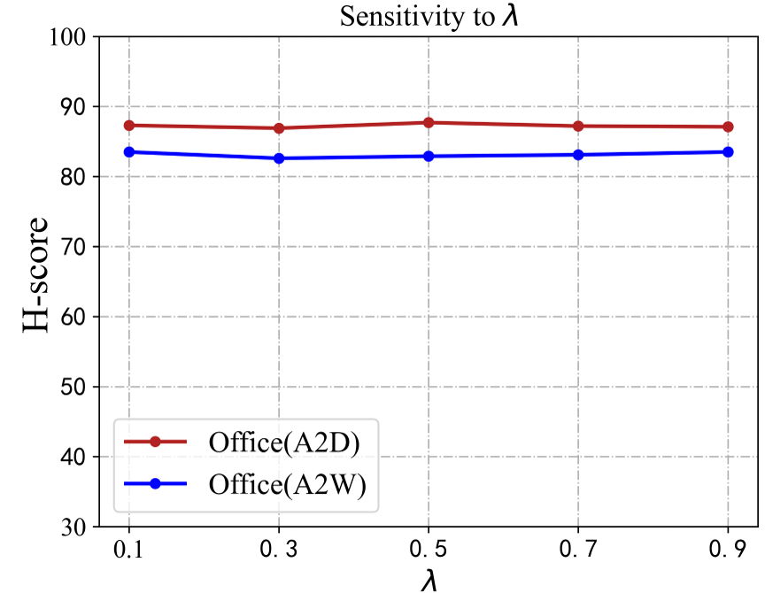
There is only one hyper-parameter $\lambda$ in the loss items. To show the sensitivity of $\lambda$ in the total loss, we conducted experiments on Office-31 (A$2$D and D$2$A) with the OPDA setting. Fig. 11(b) shows that our method has a highly stable performance over different values of $\lambda$.

References

- [1] Y. Ganin and V. Lempitsky, “Unsupervised domain adaptation by backpropagation,” in International conference on machine learning. PMLR, 2015, pp. 1180–1189.
- [2] G. Kang, L. Jiang, Y. Yang, and A. G. Hauptmann, “Contrastive adaptation network for unsupervised domain adaptation,” in Proceedings of the IEEE/CVF conference on computer vision and pattern recognition, 2019, pp. 4893–4902.
- [3] M. Long, H. Zhu, J. Wang, and M. I. Jordan, “Unsupervised domain adaptation with residual transfer networks,” arXiv preprint arXiv:1602.04433, 2016.
- [4] N. Xiao and L. Zhang, “Dynamic weighted learning for unsupervised domain adaptation,” in Proceedings of the IEEE/CVF conference on computer vision and pattern recognition, 2021, pp. 15 242–15 251.
- [5] K. Saito and K. Saenko, “Ovanet: One-vs-all network for universal domain adaptation,” arXiv preprint arXiv:2104.03344, 2021.
- [6] H. Liu, Z. Cao, M. Long, J. Wang, and Q. Yang, “Separate to adapt: Open set domain adaptation via progressive separation,” in Proceedings of the IEEE/CVF Conference on Computer Vision and Pattern Recognition, 2019, pp. 2927–2936.
- [7] B. Gong, K. Grauman, and F. Sha, “Connecting the dots with landmarks: Discriminatively learning domain-invariant features for unsupervised domain adaptation,” in International Conference on Machine Learning. PMLR, 2013, pp. 222–230.
- [8] Y. Zou, Z. Yu, B. Kumar, and J. Wang, “Unsupervised domain adaptation for semantic segmentation via class-balanced self-training,” in Proceedings of the European conference on computer vision (ECCV), 2018, pp. 289–305.
- [9] J. Na, H. Jung, H. J. Chang, and W. Hwang, “Fixbi: Bridging domain spaces for unsupervised domain adaptation,” in Proceedings of the IEEE/CVF Conference on Computer Vision and Pattern Recognition, 2021, pp. 1094–1103.
- [10] Z. Cao, L. Ma, M. Long, and J. Wang, “Partial adversarial domain adaptation,” in Proceedings of the European Conference on Computer Vision (ECCV), 2018, pp. 135–150.
- [11] Z. Cao, K. You, M. Long, J. Wang, and Q. Yang, “Learning to transfer examples for partial domain adaptation,” in Proceedings of the IEEE/CVF Conference on Computer Vision and Pattern Recognition, 2019, pp. 2985–2994.
- [12] J. Zhang, Z. Ding, W. Li, and P. Ogunbona, “Importance weighted adversarial nets for partial domain adaptation,” in Proceedings of the IEEE conference on computer vision and pattern recognition, 2018, pp. 8156–8164.
- [13] J. Liang, Y. Wang, D. Hu, R. He, and J. Feng, “A balanced and uncertainty-aware approach for partial domain adaptation,” in Computer Vision–ECCV 2020: 16th European Conference, Glasgow, UK, August 23–28, 2020, Proceedings, Part XI 16. Springer, 2020, pp. 123–140.
- [14] P. Panareda Busto and J. Gall, “Open set domain adaptation,” in Proceedings of the IEEE International Conference on Computer Vision, 2017, pp. 754–763.
- [15] K. Saito, S. Yamamoto, Y. Ushiku, and T. Harada, “Open set domain adaptation by backpropagation,” in Proceedings of the European Conference on Computer Vision (ECCV), 2018, pp. 153–168.
- [16] G. Li, G. Kang, Y. Zhu, Y. Wei, and Y. Yang, “Domain consensus clustering for universal domain adaptation,” in IEEE/CVF Conference on Computer Vision and Pattern Recognition (CVPR), 2021.
- [17] B. Fu, Z. Cao, M. Long, and J. Wang, “Learning to detect open classes for universal domain adaptation,” in European Conference on Computer Vision. Springer, 2020, pp. 567–583.
- [18] S. Bucci, M. R. Loghmani, and T. Tommasi, “On the effectiveness of image rotation for open set domain adaptation,” in European Conference on Computer Vision. Springer, 2020, pp. 422–438.
- [19] Y. Wang, L. Zhang, R. Song, H. Li, P. L. Rosin, and W. Zhang, “Exploiting inter-sample affinity for knowability-aware universal domain adaptation,” International Journal of Computer Vision, vol. 132, no. 5, pp. 1800–1816, 2024.
- [20] K. Saito, D. Kim, S. Sclaroff, and K. Saenko, “Universal domain adaptation through self supervision,” arXiv preprint arXiv:2002.07953, 2020.
- [21] L. Chen, Y. Lou, J. He, T. Bai, and M. Deng, “Geometric anchor correspondence mining with uncertainty modeling for universal domain adaptation,” in Proceedings of the IEEE/CVF Conference on Computer Vision and Pattern Recognition, 2022, pp. 16 134–16 143.
- [22] Z. Cao, M. Long, J. Wang, and M. I. Jordan, “Partial transfer learning with selective adversarial networks,” in Proceedings of the IEEE conference on computer vision and pattern recognition, 2018, pp. 2724–2732.
- [23] Z. Wang, B. Liu, S. Chen, S. Ma, L. Xue, and H. Zhao, “A manifold proximal linear method for sparse spectral clustering with application to single-cell rna sequencing data analysis,” INFORMS Journal on Optimization, vol. 4, no. 2, pp. 200–214, 2022.
- [24] Q. Feng, G. Kang, H. Fan, and Y. Yang, “Attract or distract: Exploit the margin of open set,” in Proceedings of the IEEE/CVF International Conference on Computer Vision, 2019, pp. 7990–7999.
- [25] H. Gao, Y. Li, K. Long, M. Yang, and Y. Shen, “A survey for foundation models in autonomous driving,” arXiv preprint arXiv:2402.01105, 2024.
- [26] Z. Wang, K. Balasubramanian, S. Ma, and M. Razaviyayn, “Zeroth-order algorithms for stochastic nonconvex minimax problems with improved complexities,” in Workshop on “Beyond First-Order Methods in Machine Learning Systems” hosted by the 38th International Conference on Machine Learning, 2021.
- [27] K. You, M. Long, Z. Cao, J. Wang, and M. I. Jordan, “Universal domain adaptation,” in Proceedings of the IEEE/CVF conference on computer vision and pattern recognition, 2019, pp. 2720–2729.
- [28] I. Golan and R. El-Yaniv, “Deep anomaly detection using geometric transformations,” Advances in neural information processing systems, vol. 31, 2018.
- [29] S. Wang, Y. Zeng, X. Liu, E. Zhu, J. Yin, C. Xu, and M. Kloft, “Effective end-to-end unsupervised outlier detection via inlier priority of discriminative network,” Advances in neural information processing systems, vol. 32, 2019.
- [30] K. Lee, K. Lee, H. Lee, and J. Shin, “A simple unified framework for detecting out-of-distribution samples and adversarial attacks,” Advances in neural information processing systems, vol. 31, 2018.
- [31] S. Pidhorskyi, R. Almohsen, and G. Doretto, “Generative probabilistic novelty detection with adversarial autoencoders,” Advances in neural information processing systems, vol. 31, 2018.
- [32] C. Liu, X. Zhou, Y. Wu, R. Yang, L. Zhai, Z. Jia, and Y. Liu, “Graph neural networks in eeg-based emotion recognition: a survey,” arXiv preprint arXiv:2402.01138, 2024.
- [33] S. Liang, Y. Li, and R. Srikant, “Enhancing the reliability of out-of-distribution image detection in neural networks,” arXiv preprint arXiv:1706.02690, 2017.
- [34] D. Hendrycks and K. Gimpel, “A baseline for detecting misclassified and out-of-distribution examples in neural networks,” arXiv preprint arXiv:1610.02136, 2016.
- [35] Z. Chen, J. Wang, H. Wang, Y. Yao, H. Deng, J. Peng, X. Li, Z. Wang, X. Chen, W. Xiong et al., “Machine learning reveals sex differences in clinical features of acute exacerbation of chronic obstructive pulmonary disease: A multicenter cross-sectional study,” Frontiers in Medicine, vol. 10, p. 1105854, 2023.
- [36] Q. Yu and K. Aizawa, “Unsupervised out-of-distribution detection by maximum classifier discrepancy,” in Proceedings of the IEEE/CVF international conference on computer vision, 2019, pp. 9518–9526.
- [37] Y. Sun, Y. Ming, X. Zhu, and Y. Li, “Out-of-distribution detection with deep nearest neighbors,” in International Conference on Machine Learning. PMLR, 2022, pp. 20 827–20 840.
- [38] D. Hendrycks, M. Mazeika, S. Kadavath, and D. Song, “Using self-supervised learning can improve model robustness and uncertainty,” Advances in neural information processing systems, vol. 32, 2019.
- [39] Y. Gong, F. Du, Y. Yao, H. Wang, X. Wang, W. Xiong, Q. Wang, G. He, L. Chen, H. Du et al., “Clinical characteristics of overweight patients with acute exacerbation chronic obstructive pulmonary disease (aecopd),” The Clinical Respiratory Journal, vol. 18, no. 8, p. e70001, 2024.
- [40] A. Vyas, N. Jammalamadaka, X. Zhu, D. Das, B. Kaul, and T. L. Willke, “Out-of-distribution detection using an ensemble of self supervised leave-out classifiers,” in Proceedings of the European Conference on Computer Vision (ECCV), 2018, pp. 550–564.
- [41] K. Lee, H. Lee, K. Lee, and J. Shin, “Training confidence-calibrated classifiers for detecting out-of-distribution samples,” arXiv preprint arXiv:1711.09325, 2017.
- [42] J. Ren, P. J. Liu, E. Fertig, J. Snoek, R. Poplin, M. Depristo, J. Dillon, and B. Lakshminarayanan, “Likelihood ratios for out-of-distribution detection,” Advances in neural information processing systems, vol. 32, 2019.
- [43] X. Zhou, C. Liu, L. Zhai, Z. Jia, C. Guan, and Y. Liu, “Interpretable and robust ai in eeg systems: A survey,” arXiv preprint arXiv:2304.10755, 2023.
- [44] Z. Wang, “Nonconvex stochastic nested optimization via stochastic admm,” arXiv preprint arXiv:1911.05167, 2019.
- [45] G. Shalev, Y. Adi, and J. Keshet, “Out-of-distribution detection using multiple semantic label representations,” Advances in Neural Information Processing Systems, vol. 31, 2018.
- [46] Y.-C. Hsu, Y. Shen, H. Jin, and Z. Kira, “Generalized odin: Detecting out-of-distribution image without learning from out-of-distribution data,” in Proceedings of the IEEE/CVF Conference on Computer Vision and Pattern Recognition, 2020, pp. 10 951–10 960.
- [47] Z. Liu, Z. Miao, X. Zhan, J. Wang, B. Gong, and S. X. Yu, “Large-scale long-tailed recognition in an open world,” in Proceedings of the IEEE/CVF Conference on Computer Vision and Pattern Recognition, 2019, pp. 2537–2546.
- [48] L. Neal, M. Olson, X. Fern, W.-K. Wong, and F. Li, “Open set learning with counterfactual images,” in Proceedings of the European Conference on Computer Vision (ECCV), 2018, pp. 613–628.
- [49] R. Yoshihashi, W. Shao, R. Kawakami, S. You, M. Iida, and T. Naemura, “Classification-reconstruction learning for open-set recognition,” in Proceedings of the IEEE/CVF Conference on Computer Vision and Pattern Recognition, 2019, pp. 4016–4025.
- [50] C. Wang, M. Li, J. He, Z. Wang, E. Darzi, Z. Chen, J. Ye, T. Li, Y. Su, J. Ke et al., “A survey for large language models in biomedicine,” arXiv preprint arXiv:2409.00133, 2024.
- [51] M. Liu, Z. Di, J. Wei, Z. Wang, H. Zhang, R. Xiao, H. Wang, J. Pang, H. Chen, A. Shah et al., “Automatic dataset construction (adc): Sample collection, data curation, and beyond,” arXiv preprint arXiv:2408.11338, 2024.
- [52] K. Saito, K. Watanabe, Y. Ushiku, and T. Harada, “Maximum classifier discrepancy for unsupervised domain adaptation,” in Proceedings of the IEEE conference on computer vision and pattern recognition, 2018, pp. 3723–3732.
- [53] Y. Wang, G. Huang, S. Song, X. Pan, Y. Xia, and C. Wu, “Regularizing deep networks with semantic data augmentation,” IEEE Transactions on Pattern Analysis and Machine Intelligence, 2021.
- [54] J. N. Kundu, N. Venkat, R. V. Babu et al., “Universal source-free domain adaptation,” in Proceedings of the IEEE/CVF Conference on Computer Vision and Pattern Recognition, 2020, pp. 4544–4553.
- [55] A. Paszke, S. Gross, F. Massa, A. Lerer, J. Bradbury, G. Chanan, T. Killeen, Z. Lin, N. Gimelshein, L. Antiga et al., “Pytorch: An imperative style, high-performance deep learning library,” Advances in neural information processing systems, vol. 32, pp. 8026–8037, 2019.
- [56] K. Saenko, B. Kulis, M. Fritz, and T. Darrell, “Adapting visual category models to new domains,” in European conference on computer vision. Springer, 2010, pp. 213–226.
- [57] X. Peng, Q. Bai, X. Xia, Z. Huang, K. Saenko, and B. Wang, “Moment matching for multi-source domain adaptation,” in Proceedings of the IEEE/CVF International Conference on Computer Vision, 2019, pp. 1406–1415.
- [58] X. Peng, B. Usman, N. Kaushik, J. Hoffman, D. Wang, and K. Saenko, “Visda: The visual domain adaptation challenge,” arXiv preprint arXiv:1710.06924, 2017.
- [59] K. He, X. Zhang, S. Ren, and J. Sun, “Deep residual learning for image recognition,” in Proceedings of the IEEE conference on computer vision and pattern recognition, 2016, pp. 770–778.
- [60] J. Deng, W. Dong, R. Socher, L.-J. Li, K. Li, and L. Fei-Fei, “Imagenet: A large-scale hierarchical image database,” in 2009 IEEE conference on computer vision and pattern recognition. Ieee, 2009, pp. 248–255.
- [61] L. Van der Maaten and G. Hinton, “Visualizing data using t-sne.” Journal of machine learning research, vol. 9, no. 11, 2008.
- [62] K. Simonyan and A. Zisserman, “Very deep convolutional networks for large-scale image recognition,” arXiv preprint arXiv:1409.1556, 2014.