Age of Information: Can CR-NOMA Help?

AoI indicates the freshness of the updates successfully delivered to the base station and can be defined as follows. At time $t$, denote by $T_{m}(t)$ the generation time of the freshest update successfully delivered from ${\rm U}_{m}$ to the base station. Therefore, ${\rm U}_{m}$’s instantaneous AoI is defined as follows [1]:

The normalized overall average AoI of the considered network is given by

When data is generated has significant impact on the AoI, and the following two types of data generation are considered in this paper:

CR-NOMA can be used as an add-on to TDMA to improve the freshness of the data collected in the network, as explained in the following. To reduce system complexity, the following simple user pairing scheme is considered. In particular, ${\rm U}_{m}$ and ${\rm U}_{m^{\prime}}$, where $1\leq m\leq\frac{M}{2}$ and $m^{\prime}=m+\frac{M}{2}$, are paired together to share the spectrum, and are allowed to transmit simultaneously in the $m$-th and the $m^{\prime}$-th time slots of each frame ¹¹ 1 For illustrative purposes, it is assumed that $M$ is an even number, but the proposed protocol can be straightforwardly extended to the case with an odd number of users, e.g., one of the users can be simply served by TDMA. .

The aim of CR-NOMA transmission is to increase the likelihood for each user to deliver one update to the base station every $MT$ s, compared to TDMA. Depending on the used data generation model, the application of CR-NOMA transmission is slightly different. In brief, for GAW, ${\rm U}_{m}$ and ${\rm U}_{m^{\prime}}$ use the $m$-th and the $m^{\prime}$-th time slots of each frame for their first tries for updating, respectively, as shown in Fig. 2(a). If their first tries are not successful, ${\rm U}_{m}$ uses the $m^{\prime}$-th time slot of the current frame, and ${\rm U}_{m}$ uses the $m$-th time slot of the next frame for retransmission. For GAR, both the users use the $m$-th time slot for their first tries and the $m^{\prime}$-th time slot for their second tries, as shown in Fig. 2(b). The details of CR-NOMA transmission are provided as follows.

The AoI realized for TDMA can be straightforwardly analyzed as follows. Without loss generality, we focus on ${\rm U}_{m}$’s average AoI realized for TDMA, denoted by $\bar{\Delta}^{T}_{m}$. Further denote the number of frames between the $(j-1)$-th and the $j$-th successful updates by $x_{j}$. In Fig. 3(a), an example with $x_{j}=2$ is shown. Therefore, finding the average AoI for TDMA is equivalent to find the area of the shaded region in Fig. 3(a), denoted by $Q_{j}$, which means that $\bar{\Delta}_{m}^{T}$ can be expressed as follows:

where $J$ denotes the total number of the successful updates, $Q_{j}=x_{j}MT^{2}+\frac{1}{2}x_{j}^{2}M^{2}T^{2}$, $\mathcal{E}\{X\}=\underset{J\rightarrow\infty}{\lim}\frac{1}{J}\sum^{J}_{j=1}x_{j}$, and $\mathcal{E}\{X^{2}\}=\underset{J\rightarrow\infty}{\lim}\frac{1}{J}\sum^{J}_{j=1}x_{j}^{2}$. Since the users’ channel gains are assumed to be i.i.d., $x_{j}$ follows the geometric distribution, i.e., the probability mass function of $x_{j}$ is given by $\mathbb{P}(X=x_{j})=p_{e}^{x_{j}-1}(1-p_{e})$, where $p_{e}$ denotes the probability for the event that a user fails to deliver an update in a time slot with $T$ s. By using the assumptions that each update contains $N$ bits and the users’ channel gains are complex Gaussian distributed, $p_{e}=\mathbb{P}(T\log(1+P|h_{m}^{i,m^{\prime}}|^{2})\leq N)=1-e^{-\frac{\epsilon}{P}}$, where $\epsilon=2^{\frac{N}{T}}-1$. As a result, the normalized average AoI achieved by TDMA can be obtained as follows:

where the first step follows by the fact that the users experience the same AoI in TDMA, and the second step follows by using the mean and the variance of the geometric distribution.

The analysis of the AoI realized with CR-NOMA is more challenging than that for TDMA. The reason is that each user has two transmission opportunities in each TDMA frame, which means that the time interval between the two adjacent successful updates is not always a multiple of $MT$. The following lemma provides a closed-form expression for the AoI realized by CR-NOMA.

Based on the closed-form expression of the AoI given in Lemma 1, an asymptotic analysis can be carried out to obtain an insightful understanding of the impact of NOMA on the AoI. For example, consider the following high SNR scenario, $P^{S}=P\rightarrow\infty$, which means that $p_{m}\approx 1-\frac{\epsilon}{P}$. $p_{m^{\prime}}$ can be approximated as follows:

Furthermore, $p_{0}$ can be approximated at high SNR as follows:

By using the high-SNR approximations of $p_{0}$, $p_{m}$ and $p_{m^{\prime}}$, the AoI achieved by CR-NOMA can be approximated as follows:

where step 1 follows by the fact that $p_{m}\gg p_{m^{\prime}}$ at high SNR.

On the other hand, the AoI realized by TDMA can be approximated at high SNR as follows:

Comparing the AoI shown in (10) and (11), the following corollary can be obtained.

Remark 1: The conclusion shown in Corollary 1 is expected since, at high SNR, ${\rm U}_{m}$’s first try, i.e., its transmission in the $m$-th time slot, is almost guaranteed to be successful. Therefore, retransmission is not needed at high SNR, and CR-NOMA is reduced to TDMA, which explains why the two protocols achieve the same AoI at high SNR. However, it is important to point out that the use of CR-NOMA can result in a significant performance gain over TDMA in the low SNR regime, as shown in the simulation section.

Remark 2: The use of CR-NOMA means that a user may need to transmit two times every $MT$ s, which can cause a higher energy consumption than for TDMA. In order to avoid this drawback, prior to its transmit time slot, a user can first calculate its data rate supported by CR-NOMA, and transmit only if this data rate is sufficient to deliver its update. This implementation requires that each user knows its own channel state information (CSI) as well as that of its partner. This CSI assumption can be realized as follows. The base station first broadcasts a pilot signal before a time slot, and then each user carries out channel estimation individually. In addition, the CSI of each user’s partner can be obtain either via device-to-device communication between the partners or via a dedicated control channel.

To be consistent with the illustration of Fig. 4, ${\rm U}_{m^{\prime}}$’s AoI is considered, but ${\rm U}_{m}$’s AoI can be analyzed similarly. As shown in Fig. 4(a), in TDMA, ${\rm U}_{m^{\prime}}$ is allowed to use the $m^{\prime}$-th time slot only, i.e., its transmit time slot ends at $t_{i}^{{m^{\prime}}+1}$ in the $i$-th frame, where it is important to point out that its update is generated at $t_{i}^{1}$. Again denote by $x_{j}$ the number of frames between the $(j-1)$-th and the $j$-th successful updates, where an example with $x_{j}=2$ is shown in Fig. 4.

Similar to the GAW case, the time span between the two adjacent successful updates is $x_{j}MT$; however, the AoI does not drop to $T$ whenever there is a successful update. Instead, the AoI drops to ${m^{\prime}}T$ only, because ${\rm U}_{m^{\prime}}$’s update is generated at the beginning of the frame. Therefore, ${\rm U}_{m^{\prime}}$’s averaged AoI achieved by TDMA is given by

By using steps similar to those in Section III-A, ${\rm U}_{m^{\prime}}$’s averaged AoI achieved by TDMA for the GAR model can be obtained as follows:

Comparing (5) to (13), one can find that with the GAR model, the users experience a larger AoI, which is mainly due to the access delay, i.e., a user generates its update at the beginning of one frame but has to wait for its turn to deliver the update.

The AoI realized by CR-NOMA in the GAR case is challenging to analyze due to the fact that a user’s instantaneous AoI does not always drop to the same value, which is different from the GAW case. In particular, in the GAW case, a user’s instantaneous AoI is always reduced to $T$, regardless which time slot is used for update delivery. However, in the GAR case, if ${\rm U}_{m}$ successfully delivers its update in the $m$-th time slot of a frame, its instantaneous AoI drops to $mT$, whereas its instantaneous AoI drops to $m^{\prime}T$ if the transmission in the $m^{\prime}$-th time slot is successful. What makes the AoI analysis more complicated is that the calculation of the shaded region $Q_{j}^{m^{\prime}}$ shown in Fig. 4 does not only depend on which time slot is used for the $(j-1)$-th successful update but also on which time slot is used for the $j$-th successful update. Furthermore, whether a user can successfully deliver its update to the base station is also affected by its partner’s transmission strategy, as discussed in Section II-C. The following lemma provides a closed-form expression for the AoI realized by CR-NOMA in the GAR case.

Although the AoI expression shown in Lemma 2 is lengthy and complicated, it can be used to obtain an insightful understanding of the impact of NOMA on the AoI. Let us consider the high SNR scenario, i.e., $P^{S}=P\rightarrow\infty$. Because the use of NOMA reduces the access delay for ${\rm U}_{m^{\prime}}$, it is expected that ${\rm U}_{m^{\prime}}$’s AoI experience for TDMA and NOMA will be significantly different, and hence we focus on ${\rm U}_{m^{\prime}}$’s AoI in the following.

With some straightforward algebraic manipulations, at high SNR, the following approximations can be obtained: $p_{0m^{\prime}}\approx\frac{\epsilon}{1+\epsilon}\frac{\epsilon}{P}$, $p_{mm^{\prime}}\approx\frac{1-\frac{\epsilon}{P}}{1+\epsilon}$, and $p_{m^{\prime}m^{\prime}}\approx\frac{\epsilon}{1+\epsilon}\left(1-\frac{\epsilon}{P}\right)$, which lead to the following approximation: $p_{mm^{\prime}}+p_{m^{\prime}m^{\prime}}\approx 1-\frac{\epsilon}{P}$. On the one hand, by using these approximations, the first term in (14), $\Delta_{m^{\prime},0}$, can be approximated at high SNR as follows:

On the other hand, the second term in (14), $\Delta(p_{0m^{\prime}},p_{mm^{\prime}},p_{m^{\prime}m^{\prime}})$, can be approximated as follows:

Therefore, ${\rm U}_{m^{\prime}}$’s AoI can be approximated at high SNR as follows:

where the last step follows by using the fact that $m^{\prime}=m+\frac{M}{2}$.

Recall that ${\rm U}_{m^{\prime}}$’s AoI for TDMA can be approximated at high SNR as follows: $m^{\prime}T+\frac{MT}{2}$. Therefore, the difference between ${\rm U}_{m^{\prime}}$’s AoI for TDMA and NOMA, denoted by $D_{m^{\prime}}$, is given by

which means that ${\rm U}_{m^{\prime}}$ experiences less AoI for NOMA than for TDMA.

In order to find a high-SNR approximation for $\bar{\Delta}_{m}^{N}$, the following approximations can be obtained first: $\tau\approx\frac{\epsilon}{P}$, $p_{mm}\approx 1-\frac{\epsilon}{P}$, $p_{m^{\prime}m}\approx\frac{\epsilon}{P}\frac{1-\frac{\epsilon}{P}}{1+\epsilon}+\frac{\epsilon}{P}$, and $p_{0m}\approx\frac{\epsilon}{P}\frac{\epsilon}{1+\epsilon}$. By applying these approximations and also using steps similar to those used for approximating $\bar{\Delta}_{m^{\prime}}^{N}$, ${\rm U}_{m}$’s AoI can be approximated at high SNR as follows:

which is identical to the case of TDMA. Therefore, the following corollary can be obtained.

Remark 3: For ${\rm U}_{m^{\prime}}$, the performance gain of NOMA over TDMA at high SNR is due to the fact that the use of NOMA reduces the access delay, which is particularly important in the GAR case. Recall that in the GAR case, a user’s update is generated at the beginning of the TDMA frame, which means that a user which is scheduled later in the frame suffers from a larger AoI. The use of NOMA always ensures that ${\rm U}_{m^{\prime}}$ does not have to wait until the $m^{\prime}$-th time slot, but can transmit earlier, i.e., in the $m$-th time slot, which leads to the AoI reduction stated in Corollary 2. We note that the use of NOMA does not improve ${\rm U}_{m}$’s access delay, which is the reason why ${\rm U}_{m}$’s AoIs for TDMA and NOMA are identical at high SNR.

Remark 4: We further note that the AoI reduction due to the use of CR-NOMA is important to improve user fairness. For example, two user which are scheduled in the first and the last time slots of a frame experience significantly different AoI for TDMA, but the use of CR-NOMA can reduce the difference between the users’ AoI experience.

Recall that for the GAW model, each user generates a new update at the beginning of its transmit time slot. The impact of the different transmission protocols on the AoI is investigated in Fig. 5 by assuming that there are $M=8$ users, i.e., there are $8$ time slots in each TDMA frame. As can be seen from the two subfigures in Fig. 5, the AoI achieved by the proposed NOMA transmission protocol can be significantly lower than that for TDMA. For example, for $R=1$ bits/s/Hz, $T=1.5$ s, and a transmit SNR of $0$ dB, the AoI realized with TDMA is around $28$, and the AoI achieved by CR-NOMA is just $20$, which means that the use of CR-NOMA yields more than a one-quarter reduction compared to TDMA. However, at high SNR, Fig. 5 shows that TDMA and NOMA yield the same AoI, which confirms Corollary 1. We also note that both subfigures in Fig. 5 verify the accuracy of the analytical results presented in Lemma 1 as well as the approximation result developed in (10).

Fig. 5 also shows the impact of $R$ on the AoI performance of the considered transmission protocols. In particular, by comparing Fig. 5(a) and Fig. 5(b), one can observe that increasing $R$ increases the AoI for both transmission protocols. Recall that increasing $R$ for given value of $T$ means that there are more bits contained in each update, which makes transmission failures more likely and hence increases the AoI. We note that the performance gain of NOMA over TDMA becomes larger for larger $R$. For example, for $T=1.5$ s and a transmit SNR of $0$ dB, the performance gain of NOMA over TDMA if $R=0.5$ bits/s/Hz is $3$, and this performance gain can be increased to almost $8$ if $R=1$ bits/s/Hz. The subfigures in Fig. 5 also show that the AoI realized by the considered protocols increases with $T$, since increasing $T$ for given $R$ means that there are more bits contained in each update.

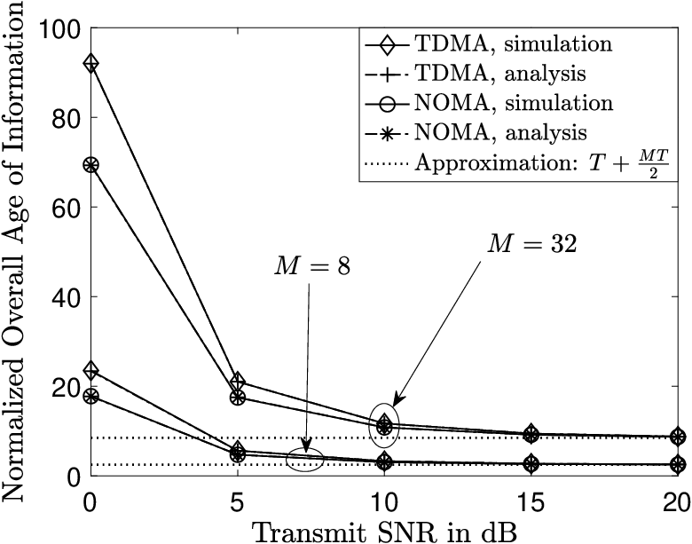
In Fig. 6, the impact of the number of users, $M$, on the AoI achieved by the considered transmission protocols is studied. As can be seen from the figure, by increasing $M$, the AoI is increased for both transmission protocols. This observation is expected since with more users in the network, each user has to wait for a longer period of time to be served. In addition, one can also observe that the performance gain of the proposed NOMA protocol over TDMA increases as the number of users, $M$, increases. For example, the performance gap between the two protocols is $5$ for $M=8$, and increases to $25$ for $M=32$. This observation means that the proposed NOMA protocol is particularly useful for reducing the AoI of networks with massive connectivity, which is a key use case of the 6G system.

Recall that for the GAR model, each user generates its update at the beginning of each TDMA frame, instead of each time slot as in the GAW case. In Fig. 7, the impact of the NOMA transmission protocol on the users’ individual AoI is studied for the GAR model. In particular, Fig. 7(a) focuses on ${\rm U}_{m}$’s individual AoI achieved by the two considered transmission protocols, $1\leq m\leq\frac{M}{2}$. Unlike for the GAW model, different users experience different AoIs for the GAR model, i.e., ${\rm U}_{m}$’s AoI is larger than that of ${\rm U}_{i}$’s, $m>i$. This observation is expected since ${\rm U}_{m}$’s instantaneous AoI can drop to $mT$ at most, whereas ${\rm U}_{i}$’s instantaneous AoI can drop to $iT$. Fig. 7(a) also shows that for ${\rm U}_{m}$, the performance gain of NOMA over TDMA is similar to that for the GRW case, e.g., the use of NOMA yields a significant performance gain at low SNR but achieves the same AoI as TDMA at high SNR. This performance gain at low SNR is due to the fact that ${\rm U}_{m}$ has a second chance for transmission in each frame, whereas for TDMA, ${\rm U}_{m}$ has to rely on a single time slot for its updates.

Fig. 7(b) focuses on ${\rm U}_{m^{\prime}}$’s individual AoI achieved for the two transmission protocols. As can be seen from the figure, NOMA outperforms TDMA in all SNR regimes. The reason for this superior performance can be explained as follows. Recall that for TDMA, ${\rm U}_{m^{\prime}}$ has to rely on the $m^{\prime}$-th time slot only for sending its update to the base station. The use of the proposed NOMA protocol has two advantages for reducing the AoI. One is that the use of NOMA offers the user two chances to transmit in each TDMA time frame. The other is that the proposed NOMA protocol can schedule ${\rm U}_{m^{\prime}}$ to transmit earlier, i.e., completing its update in the $m$-th time slot, instead of waiting for the $m^{\prime}$-th time slot as for TDMA. The latter is crucial for NOMA to outperform TDMA in the high SNR regime, as indicated by Corollary 2. Furthermore, we note that the subfigures of Fig. 7 demonstrate the accuracy of the developed analytical results shown in Lemma 2.

In Fig. 8, the individual AoI experienced by ${\rm U}_{m}$ and ${\rm U}_{m^{\prime}}$ is compared. As can be seen from the figure, for the TDMA transmission protocol, ${\rm U}_{m^{\prime}}$’s AoI is much larger than that of ${\rm U}_{m}$, which is due to the fact that ${\rm U}_{m^{\prime}}$ has to wait for the $m^{\prime}$-th time slot to deliver its update and hence experiences large access delays. By using the proposed NOMA protocol, the difference between the two users’ AoI can be reduced significantly. For example, at high SNR, the difference between the two users’ AoI is $2$ with TDMA, and can be halved by applying NOMA. Therefore, the use of NOMA can effectively reduce the difference between the users’ AoI and hence improve user fairness, as discussed in Remark 4. We also note that Fig. 8 demonstrates the accuracy of the high SNR approximations developed in Section IV-B.

In Fig. 9, the normalized overall AoI is used as the metric to study the performance of the proposed NOMA transmission protocol with the GAR model. We note that for the GAW model, the proposed NOMA protocol has the limitation that it can outperform TDMA in the low SNR regime only, as shown in Figs. 5 and 6. Compared to Figs. 5 and 6, Fig. 9 shows that the proposed NOMA protocol can always outperform TDMA and realize a smaller overall AoI in all SNR regimes. The performance gain of NOMA over TDMA is significant for small $R$, and is reduced by increasing $R$, as shown in the two subfigures of Fig. 9. Furthermore, Fig. 9 also demonstrates that the performance gain of NOMA over TDMA increases as the number of the users, $M$, increases, which is consistent with the observations related to Fig. 6.

References

- [1] Y. Sun, E. Uysal-Biyikoglu, R. D. Yates, C. E. Koksal, and N. B. Shroff, “Update or wait: How to keep your data fresh,” IEEE Trans. Inform. Theory, vol. 63, no. 11, pp. 7492–7508, Nov. 2017.
- [2] S. Kaul, R. Yates, and M. Gruteser, “Real-time status: How often should one update?” in Proc. IEEE INFOCOM, Orlando, FL, USA, May 2012.
- [3] M. A. Abd-Elmagid, N. Pappas, and H. S. Dhillon, “On the role of age of information in the Internet of Things,” IEEE Commun. Mag., vol. 57, no. 12, pp. 72–77, Dec. 2019.
- [4] X. Wu, J. Yang, and J. Wu, “Optimal status update for age of information minimization with an energy harvesting source,” IEEE Trans. Green Commun. and Net., vol. 2, no. 1, pp. 193–204, Mar. 2018.
- [5] R. D. Yates, Y. Sun, D. R. Brown, S. K. Kaul, E. Modiano, and S. Ulukus, “Age of information: An introduction and survey,” IEEE J. Sel. Areas Commun., vol. 39, no. 5, pp. 1183–1210, May 2021.
- [6] X. You, C. Wang, J. Huang et al., “Towards 6G wireless communication networks: Vision, enabling technologies, and new paradigm shifts,” Sci. China Inf. Sci., vol. 64, no. 110301, pp. 1–74, Feb. 2021.
- [7] Z. Zhang, Y. Xiao, Z. Ma, M. Xiao, Z. Ding, X. Lei, G. K. Karagiannidis, and P. Fan, “6G wireless networks: Vision, requirements, architecture, and key technologies,” IEEE Veh. Tech. Mag., vol. 14, no. 3, pp. 28–41, Jul. 2019.
- [8] I. Krikidis, “Average age of information in wireless powered sensor networks,” IEEE Wireless Commun. Lett., vol. 8, no. 2, pp. 628–631, Apr. 2019.
- [9] A. A. Al-Habob, O. A. Dobre, and H. V. Poor, “Age- and correlation-aware information gathering,” IEEE Wireless Commun. Lett., vol. 11, no. 2, pp. 273–277, Feb. 2022.
- [10] M. Xie, J. Gong, S. Cai, and X. Ma, “Age-energy tradeoff for two-hop status update systems with heterogeneous truncated ARQ,” IEEE Wireless Commun. Lett., vol. 10, no. 7, pp. 1488–1492, Jul. 2021.
- [11] Y. Zheng, J. Hu, and K. Yang, “Average age of information in wireless powered relay aided communication network,” IEEE Internet of Things Journal, vol. 9, no. 13, pp. 11 311–11 323, Jul. 2022.
- [12] R. D. Yates and S. K. Kaul, “The age of information: Real-time status updating by multiple sources,” IEEE Trans. Inform. Theory, vol. 65, no. 3, pp. 1807–1827, Mar. 2019.
- [13] Y. H. Bae and J. W. Baek, “Age of information and throughput in random access-based IoT systems with periodic updating,” IEEE Wireless Commun. Lett., vol. 11, no. 4, pp. 821–825, Apr. 2022.
- [14] B. Yu and Y. Cai, “Age of information in grant-free random access with massive MIMO,” IEEE Wireless Commun. Lett., vol. 10, no. 7, pp. 1429–1433, Jul. 2021.
- [15] H. Pan and S. C. Liew, “Information update: TDMA or FDMA?” IEEE Wireless Commun. Lett., vol. 9, no. 6, pp. 856–860, Jun. 2020.
- [16] Y. Liu, S. Zhang, X. Mu, Z. Ding, R. Schober, N. Al-Dhahir, E. Hossain, and X. Shen, “Evolution of NOMA toward next generation multiple access (NGMA) for 6G,” IEEE J. Sel. Areas Commun., vol. 40, no. 4, pp. 1037–1071, Jan. 2022.
- [17] A. Maatouk, M. Assaad, and A. Ephremides, “Minimizing the age of information: NOMA or OMA?” in Proc. IEEE INFOCOM WKSHPS), Paris, France, 2019.
- [18] L. Liu, H. H. Yang, C. Xu, and F. Jiang, “On the peak age of information in NOMA IoT networks with stochastic arrivals,” IEEE Wireless Commun. Lett., vol. 10, no. 12, pp. 2757–2761, Dec. 2021.
- [19] H. Zhang, Y. Kang, L. Song, Z. Han, and H. V. Poor, “Age of information minimization for grant-free non-orthogonal massive access using mean-field games,” IEEE Trans. Commun., vol. 69, no. 11, pp. 7806–7820, Nov. 2021.
- [20] X. Feng, S. Fu, F. Fang, and F. R. Yu, “Optimizing age of information in RIS-assisted NOMA networks: A deep reinforcement learning approach,” IEEE Wireless Commun. Lett., to appear in 2022.
- [21] Z. Gao, A. Liu, C. Han, and X. Liang, “Non-orthogonal multiple access based average age of information minimization in LEO satellite-terrestrial integrated networks,” IEEE Trans. Green Commun. and Net., 2022.
- [22] H. Pan, J. Liang, S. C. Liew, V. C. M. Leung, and J. Li, “Timely information update with nonorthogonal multiple access,” IEEE Trans. Industrial Informatics, vol. 17, no. 6, pp. 4096–4106, Jun. 2021.
- [23] Q. Ren, T.-T. Chan, J. Liang, and H. Pan, “Age of information in sic-based non-orthogonal multiple access,” in Proc. IEEE WCNC, Austin, TX, USA, 2022.
- [24] Z. Ding, P. Fan, and H. V. Poor, “Impact of user pairing on 5G non-orthogonal multiple access,” IEEE Trans. Veh. Tech., vol. 65, no. 8, pp. 6010–6023, Aug. 2016.
- [25] R. E. Kim, J. Li, B. F. J. Spencer, T. Nagayama, and K. A. a. Mechitov, “Synchronized sensing for wireless monitoring of large structures,” Smart Structures and Systems, vol. 18, no. 5, pp. 885–909, May 2016.
- [26] C. Xu, Q. Xu, J. Wang, K. Wu, K. Lu, and C. Qiao, “AoI-centric task scheduling for autonomous driving systems,” in Proc. IEEE INFOCOM, London, UK, 2022.