Fact: Learning Governing Abstractions Behind Integer Sequences
Abstract
Integer sequences are of central importance to the modeling of concepts admitting complete finitary descriptions. We introduce a novel view on the learning of such concepts and lay down a set of benchmarking tasks aimed at conceptual understanding by machine learning models. These tasks indirectly assess model ability to abstract, and challenge them to reason both interpolatively and extrapolatively from the knowledge gained by observing representative examples. To further aid research in knowledge representation and reasoning, we present FACT, the Finitary Abstraction Comprehension Toolkit. The toolkit surrounds a large dataset of integer sequences comprising both organic and synthetic entries, a library for data pre-processing and generation, a set of model performance evaluation tools, and a collection of baseline model implementations, enabling the making of the future advancements with ease.
1 Introduction
Ordered lists of integers are the natural representation form for all fundamentally discrete abstractions. These arise when encountering evolutions of discrete-time phenomena, finite symmetries of visual patterns, or algorithmic progressions, where they describe the development of consecutive states of a system, automorphisms of , or program listings, respectively. Sequences of integers are also the representation of choice when linearising structured information for analysis, data compression, and communication, with often-appearing datapoints tending to be encoded in the simplest or shortest form. Testifying to their utility to accurately represent abstractions, completion and extrapolation tasks on integer sequences are a frequent part of general human intelligence and aptitude testing ([42, 31]).
It is the aim and the hope for machine learning models to identify straightforward universal abstractions explaining the training data, rather than to memorise a plethora of small classes of exemplars and interpolate when given previously unseen input. The discovery and internalisation of governing concepts, or simply the learning of underlying rules, thus sits at the centre of artificial intelligence research.
We note that many concepts may be uniquely represented by a sequence of integers naturally (e.g. the squares of the natural numbers determine the polynomial ; encodes the symmetries of a triangle), while others (such as the rotations of objects in scene) require a continuous space for a proper, scalable description. We recognise integer sequences as a general form for description of concepts completely representable with finite precision (finite in their nature; finitary) and put them at the centre of our study.
To discern the learning and understanding of these discrete abstractions from the learning of their representations in various modalities, we introduce a rich dataset of integer sequences together with a compendium of corresponding tasks that are innately related to integer sequences and well-suited to assess the levels of human-like understanding exhibited by machine learning models. Focusing solely on integer sequences, we thus set the concepts being learned apart from virtually all complexity stemming from the learning of a representation, making the learning process less resource-intensive and the interpretation of evaluation results more straightforward. An example learning programme making this distinction and proceeding to high-level abstractions is pictured in Figure 1.

Modern machine learning methods have been shown to posses the ability to comprehend (or at least pattern-match) convoluted concepts appearing in various data modalities, especially by the means of using deep learning to construct informative representations of the entities studied. In spite of working with number sequences, we take a step away from symbolic regression (which has so far dominated the notion of understanding in the area) and, tending to the trend, employ instead a multi-faceted approach in which sequences are characterised by their properties and relations to other sequences, rather than by explanatory symbolic formulas that are more readily interpretable by humans. We expand on the relationship of our work to symbolic regression in Appendix F.
Aiming at the comprehension of abstractions behind concrete representations of finitary phenomena, we unlock a new mode for evaluation of the quality of the abstractions learned. A guess, or an estimate, of the rule behind an integer sequence, which further leads to correct predictions of the sequence’s elements on previously unseen inputs, is arguably more desirable than an estimate that describes the sequence well only for inputs known in training. The fundamentally algorithmic nature of the problem of learning finitary abstractions thus makes the problem of extrapolative generalisation well-defined, and allows us to consider extrapolative generalisation performance as a criterion for model assessment.
Our contributions are:
- •
- •
complementing the above, a utility library (FACTLIB [6]) for integer sequence data processing and generation,
- •
the introduction of a variety of tasks designed to evaluate the model comprehension of conceptual patterns in integer sequences with a clearly established order of difficulty (Section 3),
- •
a battery of evaluation metrics tailored to the above tasks to appropriately assess model performance and track progress in this sub-area of knowledge representation and reasoning, and
- •
2 Dataset
As a part of FACT, we introduce a dataset consisting of over million integer sequences. The structure-giving starting point for the dataset was the data made available by the Online Encyclopedia of Integer Sequences ([39]). The OEIS is an organically grown comprehensive reference on noteworthy sequences of integers, compiled over decades to aid work in mathematical sciences. We have reviewed the OEIS4 data, set apart a suitable subset of 341,000 entries, and processed it specifically for use in machine learning, in line with the license requirements. Each entry of the dataset is now annotated by up to 18 features conveying the information about the nature, properties, and purpose of the sequence. In Figure 4, we give an overview of the result of this processing step. A full discourse on the extensive curation, refining, and automated annotation effort undertaken can be found in Appendix A.
With the encyclopedia entries aimed at a human reader, we observed that many covered their respective categories only very sparsely, relying on the associated natural language descriptions and the human ability to abstract to make the categorical connection. Our initial experiments with the baseline models (cf. Section 4) further confirmed that much of the data did not reach the critical mass of information necessary for reliable use in machine learning applications. We hence systematically extended the dataset by synthetically generated sequence branches while abiding by the structure and nature of the stem encyclopedia entries and providing carefully engineered automatic annotations wherever possible.
2.1 Synthetic Generation
Our principal inspirations were the notions of Kolmogorov complexity and Solomonoff probability [33, 20, 41]. Starting on the level of categories (cf. Figure 4), we defined a context-free grammar for each category , and then used to generate ever longer formulas, which were in turn used to generate the sequences. This was done abiding by the notion that the growing length of formulas reflects itself in increasing complexity of rules and therefore generated sequences. An example grammar, used for the production of polynomial formulas, is given in Figure 3.
For each category, a total of 500K synthetic sequences have been generated. The length of the formulas used to generate these sequences was continuously increased following a logarithmic schedule, thereby favouring shorter formulas while still ensuring the presence of sequences from longer formulas. We give all details of our generation procedure for each sequence category in Appendix B.
The combined result of the OEIS curation and the dataset extension process is therefore a large dataset seamlessly integrated into FACT and easily extensible by FACTLIB, if required by more complex tasks or larger applications.
3 Benchmark
Based on the dataset of the previous section, we propose a set of benchmarking tasks and evaluation metrics to assess a wide range of methods for their understanding of governing concepts behind evolutions of integer sequences.
3.1 Motivation
Consider the initial segment of a sequence and assume we are tasked with proposing reasonable candidates for the number that follows .
How could we go about evaluating the quality of our suggestions?
In the spirit of symbolic regression, we may choose to insist that there must be a single formula that produces the members of the sequence in order. But, even under such condition, for every suggested continuation integer there exists a degree- polynomial accommodating the continued sequence. This is despite the fact that a human would intuitively be most likely to suggest as a reasonable continuation, perhaps even justifying it by the observation that the first elements of the sequence follow the pattern of .
As described in Section 2, we have therefore set the generation methods of the synthetic part of our dataset to explicitly apply the parsimony principle by varying the length of generative formulas to control the complexity of the resulting sequences. Data generated in this manner is guaranteed to encompass sequences coming from rules of varying degrees of complexity by design, rather than by chance.
The focus on preferring shorter rules over longer ones would, however, be too artificial if employed alone. Consider the initial segment . While it is tempting to promptly claim that the numbers come from the Fibonacci sequence and that should follow, an answer arising more naturally in the context of chemistry is , as the continued sequence represents the count of all possible -carbon alkanes.
Hence, striding ahead of the symbolic regression under Occam’s razor, we add a processed part of the OEIS dataset into our evaluation procedures as an indicator of the sequences’ appeal across a multitude of scientific disciplines. Note that this is an improvement made in addition rather than in contrast to the principles for synthetic sequence generation, as many of the real-world sequences collected in OEIS do indeed obey straightforward rules.
3.2 Structure
As motivated in Section 3.1, for each benchmarking task we provide two evaluation sets: one for synthetic data and one for OEIS data. Our benchmark thus pushes for the design of machine learning models that identify simple concepts and rules (evaluation on synthetic data) but still retains enough of cross-domain generality to have practical impact in different disciplines (evaluation on OEIS).
The benchmark consists of tasks with an established order of difficulty over two dimensions: the task type and scope. We distinguish between the tasks of sequence classification, sequence similarity, next sequence part prediction, sequence continuation, and sequence unmasking – each detailed below.
In addition, we perform each task to the extent of two different scopes: within and across categories. The case of performing the task within categories is the simpler of the two setups, since the category from which the sequence originates is known in advance, and this information is thus also available at the time models are designed. Nevertheless, our baselines (cf. Section 4) are oblivious to this information and instead treat the category scope as if nothing was known about the data.
In our particular benchmarking setup, our dataset is split into four parts, namely the training, validation, synthetic test, and organic test sets. The training and validation sets consist of only synthetic sequences. The size ratios between training, validation, synthetic testing, and OEIS testing datasets are 9:1:1:1. For convenience and future reference, we make this divided-up data available as separate datasets. Nevertheless, the FACT dataset is also available in one piece, allowing users to choose their own splits or supplement their own data generated by FACTLIB, according to their needs.
3.3 Task Types
In this section we present 5 types of tasks in order of difficulty, for which we take the upper bound on the difficulty of the task instances comprising the given task. For example: Every instance of sequence continuation belongs to the set of sequence unmasking instances. But, for every instance of sequence continuation (except for the trivial one where we only begin with one number) there is an instance of unmasking that is harder. Such an instance can be formed by further asking to unmask a sequence element somewhere in the initial segment provided for continuation. Hence, the upper bound on the difficulty of sequence unmasking is strictly higher than the upper bound on the difficulty of sequence continuation.
3.3.1 Sequence Classification
The simplest task type in our benchmark is classifying in which category the sequence belongs. The chief goal of this task is to evaluate whether models can distinguish and identify general patterns in sequences, both across and within different categories. Note that category membership may not necessarily be unique. For example, a sequence can be bounded, but also periodic. For this task we use all categories that possess a synthetic counterpart within our dataset. Each sample consists of an array of integer numbers for the given sequence class. We distinguish between two task sub-types and give their objectives:
- •
One-vs-Rest (OvR). Obj. to identify whether the sequence belongs to a specified category or not. For this case, we provide a balanced dataset in each category. This is a binary classification task, and as such, we use accuracy as the evaluation metric.
- •
Multiclass classification. Obj. to predict, for every sequence, all categories to which it belongs. The performance is measured with the macro average F1 score (i.e. the mean of individual per-class F1 scores) due to inherent imbalances in our dataset.
3.3.2 Sequence Similarity
The similarity task aims to assess model ability to represent sequences in a way that reflects their similarities in type (e.g. agreeing on category membership) or properties (such as being periodic or unbounded) in the spirit of [24]. The objective is to embed sequences into an embedding space such that sequences belonging to the same category are closer to one another than to sequences of categories to whom they do not belong. We evaluate using
- •
the Recall@ score, where the candidates for a sequence are proposed by sampling sequences from each category and then ordering the category labels according to the distance of the carrier points from ; and
- •
the top- root mean squared error – the root mean squared error (RMSE) across the top similarity candidates. Given predictions of a model and ground truth , we define the top- RMSE as . In other words, given all generated predictions we report the RMSE of the prediction closest to the ground truth.
Our choice of evaluation metrics is grounded in the observation that sequences generated from similar simple rules often eventually diverge, and that to a large extent. This task generalises sequence classification.
3.3.3 Next Sequence-Part Prediction
As seen in natural language processing [10], asking a model to decide whether two sentences follow one another can be beneficial for testing of whether a model understands its inputs. Given two contiguous sub-sequences and , the objective of the next sequence-part prediction (NSPP) task is to determine whether the sub-sequence is a valid continuation of . We create a balanced dataset for this task, by using all categories of our dataset that have a synthetic counterpart. NSPP is then simply a binary classification task and the performance is measured by prediction accuracy. This task is strictly more difficult than the similarity task, since it demands that the model not only understands the key properties of the sequence but also possesses the ability to discern unlikely or unfeasible combinations of sequence parts from the feasible ones.
3.3.4 Sequence Continuation
The fourth task type in our difficulty hierarchy is to suggest the next entry in a given sequence . This task is extrapolative in its nature, and is meant to challenge model understanding beyond making a binary decision between externally provided suggestions. As such, this task demands better understanding of the rules governing sequences than next sequence-part prediction – hence it’s placement above NSPP in the difficulty hierarchy. We distinguish two sub-types of this task, namely the single-shot and multi-shot continuations, differing only in the number of candidates the model is expected to provide for the continuation. We use the root mean squared logarithmic error (RMSLE) and top- RMSE for each of the sub-types, respectively.
3.3.5 Sequence Element Unmasking
At the apex of our complexity hierarchy is the task of unmasking marked elements of a provided sequence. The sequence continuation task can be viewed as a special case of unmasking, where only the last element is masked. We consider only multi-shot unmasking and choose top- RMSE as the evaluation metric.
4 Baseline model performance
We run extensive experiments on the proposed benchmark as a starting point for further research. We consider classical machine learning methods as well as large neural networks. The experiments in this section highlight the feasibility of learning many different patterns in integer sequences, but also some of the limitations of the existing methods.
4.1 Models
To provide baselines for model performance on the above tasks, we use a total of 24 different models across our benchmarking tasks, namely 4 neural models (dense, recurrent, and convolutional networks, and transformers), 9 classical classifiers (-nearest neighbours, Gaussian naive Bayes, linear support vector machine, decision tree, random forest, gradient boosting, AdaBoost, XG Boost, dummy classifier), and 11 standard regressors (-nearest neighbours, linear regressor, ridge regressor, lasso regressor, Elastic Net, single decision tree, random forest, gradient boosting, AdaBoost, dummy regressor).
We give details on their implementations and hyperparameter settings in Appendix C.
4.2 Results
A simple overview of the performance of the baseline models can be found in Table 1. A comprehensive, detailed listing of our results, including results of evaluations on the category level, can be found in Appendix D.
| Model | Dataset | Task | ||||
|---|---|---|---|---|---|---|
| classification | next part pred. | continuation | similarity | unmasking | ||
| [F1 score] | [binary-accuracy] | [RMSLE] | [top--RMSE] | |||
| MLP | oeis | 0.33 | 0.733 | 0.597 | 0.301 | 2.918 |
| synth | 0.43 | 0.943 | 0.430 | 1.690 | 3.408 | |
| RNN | oeis | 0.37 | 0.869 | 0.603 | 0.383 | 2.944 |
| synth | 0.53 | 0.984 | 0.406 | 0.438 | 3.379 | |
| CNN | oeis | 0.22 | 0.551 | 0.733 | 0.428 | 2.440 |
| synth | 0.39 | 0.900 | 0.579 | 0.643 | 2.812 | |
| Transformer | oeis | 0.33 | 0.736 | 0.578 | 0.267 | 2.811 |
| synth | 0.44 | 0.938 | 0.395 | 0.270 | 3.091 | |
| k-Nearest Neighbours | oeis | 0.33 | – | 0.808 | – | – |
| synth | 0.41 | – | 0.486 | – | – | |
| Gaussian Naive Bayes | oeis | 0.23 | – | – | – | – |
| synth | 0.37 | – | – | – | – | |
| Support Vector Machine | oeis | 0.31 | – | – | – | – |
| synth | 0.35 | – | – | – | – | |
| Decision Tree | oeis | 0.36 | – | 0.730 | – | – |
| synth | 0.49 | – | 0.427 | – | – | |
| Random Forest | oeis | 0.34 | – | 0.730 | – | – |
| synth | 0.51 | – | 0.427 | – | – | |
| Grad.-Boosted Rand. Forest | oeis | 0.27 | – | 0.702 | – | – |
| synth | 0.40 | – | 0.484 | – | – | |
| AdaBoost | oeis | 0.31 | – | 0.842 | – | – |
| synth | 0.38 | – | 0.662 | – | – | |
| XGBoost | oeis | 0.37 | – | 0.719 | – | – |
| synth | 0.51 | – | 0.433 | – | – | |
| Elastic Net Regressor | oeis | – | – | 0.814 | – | – |
| synth | – | – | 0.716 | – | – | |
| Ridge Regressor | oeis | – | – | 0.797 | – | – |
| synth | – | – | 0.682 | – | – | |
| Lasso Regressor | oeis | – | – | 0.827 | – | – |
| synth | – | – | 0.747 | – | – | |
| Linear Regressor | oeis | – | – | 0.797 | – | – |
| synth | – | – | 0.682 | – | – | |
| Dummy | oeis | 0.50 | – | 0.923 | – | – |
| synth | 0.50 | – | 0.877 | – | – | |
4.3 Metric Interpretation
The macro-averaged F1-scores for the sequence classification task in Table 1 suggest that even the best-performing models have an average score of little over . The F1 score of can be achieved in many ways, but would for example correspond to a precision-recall performance of . In the next sequence-part prediction, the RNNs appear to be nearing the perfect accuracy score of , though some room for improvement remains to be seen in the case of the organic dataset. The root mean squared logarithmic errors of (best OEIS performance) and (best synthetic performance) that appear in the results for the continuation task correspond to uniform difference of logarithms of the same magnitude. In contrast, the two respective worst performances among the baselines models correspond to uniform difference between logarithms of .
The top- root mean squared errors are more straightforward to interpret. One would arrive at RMSE between initial sequence segments if were larger or smaller than by exactly in every one of its elements. Top--RMSEs of for the sequence similarity task therefore correspond to mean uniform difference of the same magnitude in every element when comparing the true sequence to the best fit from among the top results of the similarity search. The same metric is used for the unmasking task. In the light of the distribution of the elements of the sequences considered covering values from to several million, the performances of baseline models, especially in the similarity task, appear to be remarkably strong.
4.4 Comparative Analysis
Reviewing the results of Table 1 and further Appendix D, we note that even just the performance of baseline models on the synthetic dataset is often quite strong in absolute terms. We also notice a general trend among all models to perform better on synthetic data than on the organic OEIS sets. This is not unexpected, since the OEIS data is highly varied and comes from a large variety of sources, whereas the synthetic data is generated according to a strict, uniform procedure, thus having a more regular distribution. Nevertheless, we observe that training on synthetic data alone still yields solid performance on the organic dataset across all models.
In the classification task, RNNs and random forests achieve the best results across all categories. Unsurprisingly, RNNs very accurately identify bounded and increasing sequences, while random forests lead for modulo, prime, exponential and trigonometric sets. RNNs also show a consistent lead for the next sequence-part prediction. Transformers and CNNs dominate the results for similarity under the top- accuracy, with the exception of organic periodic functions, which are best handled by recurrent networks. Transformers alone lead in the same task when evaluating by top- RMSLE, and likewise for convolutional networks in the unmaskingtask .
The best performances for the continuation task are almost evenly split between recurrent networks and transformers, where RNNs lead for polynomial, exponential, trigonometric, and periodic sequences (transformers being the worst performers). Transformers yield the best results modulo, prime, bounded, increasing, and all sequences together.
We lay out our expectations for model performance on this benchmark, also in relation to human ability, in Appendix E.
5 Related Work
There has recently been a noticeable movement in neural network research towards understanding how DNNs learn to abstract. On the side of investigation, traditional architectures were analysed by [21] in terms of the emergence of knowledge across the network, a well-defined metric for the generalisation ability of neural networks was introduced in [11], and a methodology to assess knowledge representation in deep neural networks trained for object recognition in computer vision was proposed in [18]. The increasing interest in the learning of abstractions also prompted the incorporation of relevant inductive biases into deep neural architectures and training curricula, as was seen in concept acquisition [46, 14], with the introduction of the neural state machine [16] in computer vision, and causal abstraction analysis [2, 3, 13] in natural language inference. Further, efforts have already begun to assess the capability of models to perform abstracting visual reasoning [47, 1, 48, 7].
A common, classical, and still challenging instance of abstraction learning in the context of number sequences is the task of symbolic regression. A number of genetic programming models and purpose-specific datasets have been proposed in the field in its over 30 years of existence, and a systematising benchmark, SRBench [22], was recently introduced. It combines 130 smaller numerical datasets, both organically grown and synthetically generated, with the PMLB [26], and comes with an evaluation of a range of symbolic regression models using a newly-proposed metric. The inherent focus of the task on interpretability makes it suitable for industrial use but leads to challenges in identification of prevailing generative concepts, as two sequences originating from two distinct instances of the same rule may be best fitted by two formulas completely different in their nature.
Focusing on integer sequences, the Online Encyclopedia of Integer Sequences (OEIS) was presented in [39]. The entries of the encyclopedia come from both individual human contributors and automated mechanisms for the invention of “interesting” sequences [8]. It was used for sequence classification combining heuristics and machine learning methods in [45], for the sequence continuation task by fully-connected neural networks in [30], for digit-level sequence term regression to highlight the computational limits of neural networks in [25], and for the learning of mathematical properties of integers for use in natural language processing by training OEIS-sequence embeddings in [32]. The latest version, OEISv4, is the most comprehensive source of annotated information on integer sequences, containing over entries. The dataset has further seen use in the emergent sub-area of deep symbolic regression [23, 29, 9, 19].
Our experience shows that the OEIS data is too sparse and too closely tailored to the needs of human reader to be useful for training of machine learning models for integer sequence comprehension. It can still, however, serve as an interesting proxy of “usefulness” (such as in [8]) in model evaluation when appropriately filtered and pre-processed for that purpose.
6 Avenues for Future Work
The carrying advantage of the focus on integer sequences instead of other – potentially richer – input modalities is that we can directly interpret the performance scores of individual models as their ability to comprehend sequence-giving abstractions, and have the confidence that no model performance has been hampered by its insufficient understanding of the input representation. Here, while the models we evaluated appear to show some level of understanding of patterns underlying integer sequences, there is still significant room for improvement, especially in multi-class classification, sequence continuation across all classes, and sequence unmasking.
The results of Section 4 were all produced for a “static” mode of operation, in which all of the query data (e.g. the sequence to classify or a sequence prefix to continue) was provided to the model upfront and as a whole. A mode of operation occurring perhaps more naturally in most practical scenarios is that in which the model is active in its learning and interacts with an oracle, polling for information until it is confident that it can provide and answer. Such interactive variants can be readily formulated for all tasks in Section 3.3, but require a more sophisticated set of evaluation metrics that takes into consideration the amount of information the model requested before producing an answer. We believe that this setup deserves attention as it can provide valuable insights into model reasoning, and we aim to tackle it in our future work.
7 Conclusion
Integer sequences frequently arise as the natural representation form for finitary phenomena. Focusing on integer sequences allows us to directly address the problem of learning abstractions and removes the otherwise necessary overhead of learning modality-specific representations.
The benchmarking toolkit for integer sequences presented in this work is by design general in its purpose, aimed at fundamental understanding due to its use of integers as primitive representations, and hierarchically encompasses many of the tasks that have previously appeared isolated in the literature.
It is our hope that our work will help attract attention to the challenges of designing models that perceive logical relationships ruling over the training corpora and reason during inference, thus helping to facilitate future advancements on the frontiers of general artificial intelligence.
References
- Barrett et al. [2018] David Barrett, Felix Hill, Adam Santoro, Ari Morcos, and Timothy Lillicrap. Measuring abstract reasoning in neural networks. In International conference on machine learning, pages 511–520. PMLR, 2018.
- Beckers and Halpern [2019] Sander Beckers and Joseph Y Halpern. Abstracting causal models. In Proceedings of the aaai conference on artificial intelligence, volume 33, pages 2678–2685, 2019.
- Beckers et al. [2020] Sander Beckers, Frederick Eberhardt, and Joseph Y Halpern. Approximate causal abstractions. In Uncertainty in Artificial Intelligence, pages 606–615. PMLR, 2020.
- Belcak, Peter et al. [2022a] Belcak, Peter, Kastrati, Ard, and Schenker, Flavio. Fact benchmarking - the benchmarking baseline models of the finitary abstraction comprehension toolkit, 2022a. URL https://doi.org/10.3929/ethz-b-000565644.
- Belcak, Peter et al. [2022b] Belcak, Peter, Kastrati, Ard, and Schenker, Flavio. Fact dataset - the dataset of the finitary abstraction comprehension toolkit, 2022b. URL https://doi.org/10.3929/ETHZ-B-000562705.
- Belcak, Peter et al. [2022c] Belcak, Peter, Kastrati, Ard, and Schenker, Flavio. Factlib - the library of the finitary abstraction comprehension toolkit, 2022c. URL https://doi.org/10.3929/ethz-b-000565638.
- Chollet [2019] François Chollet. On the measure of intelligence. arXiv preprint arXiv:1911.01547, 2019.
- Colton et al. [2000] Simon Colton, Alan Bundy, and Toby Walsh. Automatic invention of integer sequences. In AAAI/IAAI, pages 558–563, 2000.
- d’Ascoli et al. [2022] Stéphane d’Ascoli, Pierre-Alexandre Kamienny, Guillaume Lample, and François Charton. Deep symbolic regression for recurrent sequences. arXiv preprint arXiv:2201.04600, 2022.
- Devlin et al. [2018] Jacob Devlin, Ming-Wei Chang, Kenton Lee, and Kristina Toutanova. Bert: Pre-training of deep bidirectional transformers for language understanding. arXiv preprint arXiv:1810.04805, 2018.
- Gain and Siegelmann [2020] Alex Gain and Hava Siegelmann. Abstraction mechanisms predict generalization in deep neural networks. In International Conference on Machine Learning, pages 3357–3366. PMLR, 2020.
- Gebru et al. [2018] Timnit Gebru, Jamie Morgenstern, Briana Vecchione, Jennifer Wortman Vaughan, Hanna Wallach, Hal Daumé III, and Kate Crawford. Datasheets for datasets. arXiv preprint arXiv:1803.09010, 2018.
- Geiger et al. [2021] Atticus Geiger, Hanson Lu, Thomas Icard, and Christopher Potts. Causal abstractions of neural networks. Advances in Neural Information Processing Systems, 34, 2021.
- Higgins et al. [2017] Irina Higgins, Nicolas Sonnerat, Loic Matthey, Arka Pal, Christopher P Burgess, Matko Bosnjak, Murray Shanahan, Matthew Botvinick, Demis Hassabis, and Alexander Lerchner. Scan: Learning hierarchical compositional visual concepts. arXiv preprint arXiv:1707.03389, 2017.
- Hochreiter and Schmidhuber [1997] Sepp Hochreiter and Jürgen Schmidhuber. Long short-term memory. Neural computation, 9:1735–80, 12 1997. doi: 10.1162/neco.1997.9.8.1735.
- Hudson and Manning [2019] Drew Hudson and Christopher D Manning. Learning by abstraction: The neural state machine. Advances in Neural Information Processing Systems, 32, 2019.
- Husain et al. [2019] Hamel Husain, Ho-Hsiang Wu, Tiferet Gazit, Miltiadis Allamanis, and Marc Brockschmidt. Codesearchnet challenge: Evaluating the state of semantic code search. arXiv preprint arXiv:1909.09436, 2019.
- Ilin et al. [2017] Roman Ilin, Thomas Watson, and Robert Kozma. Abstraction hierarchy in deep learning neural networks. In 2017 International Joint Conference on Neural Networks (IJCNN), pages 768–774. IEEE, 2017.
- Kamienny et al. [2022] Pierre-Alexandre Kamienny, Stéphane d’Ascoli, Guillaume Lample, and François Charton. End-to-end symbolic regression with transformers. arXiv preprint arXiv:2204.10532, 2022.
- Kolmogorov [1965] Andrei N Kolmogorov. Three approaches to the quantitative definition of information’. Problems of information transmission, 1(1):1–7, 1965.
- Kozma et al. [2018] Robert Kozma, Roman Ilin, and Hava T Siegelmann. Evolution of abstraction across layers in deep learning neural networks. Procedia computer science, 144:203–213, 2018.
- La Cava et al. [2021] William La Cava, Patryk Orzechowski, Bogdan Burlacu, Fabrício Olivetti de França, Marco Virgolin, Ying Jin, Michael Kommenda, and Jason H Moore. Contemporary symbolic regression methods and their relative performance. arXiv preprint arXiv:2107.14351, 2021.
- Lample and Charton [2019] Guillaume Lample and François Charton. Deep learning for symbolic mathematics. arXiv preprint arXiv:1912.01412, 2019.
- Mikolov et al. [2013] Tomas Mikolov, Kai Chen, Greg Corrado, and Jeffrey Dean. Efficient estimation of word representations in vector space. arXiv preprint arXiv:1301.3781, 2013.
- Nam et al. [2019] Hyoungwook Nam, Segwang Kim, and Kyomin Jung. Number sequence prediction problems for evaluating computational powers of neural networks. In Proceedings of the AAAI Conference on Artificial Intelligence, volume 33, pages 4626–4633, 2019.
- Olson et al. [2017] Randal S Olson, William La Cava, Patryk Orzechowski, Ryan J Urbanowicz, and Jason H Moore. Pmlb: a large benchmark suite for machine learning evaluation and comparison. BioData mining, 10(1):1–13, 2017.
- Pedregosa et al. [2011] F. Pedregosa, G. Varoquaux, A. Gramfort, V. Michel, B. Thirion, O. Grisel, M. Blondel, P. Prettenhofer, R. Weiss, V. Dubourg, J. Vanderplas, A. Passos, D. Cournapeau, M. Brucher, M. Perrot, and E. Duchesnay. Scikit-learn: Machine learning in Python. Journal of Machine Learning Research, 12:2825–2830, 2011.
- Penrose [1990] Roger Penrose. The Emperor’s New Mind: Concerning Computers, Minds, and the Laws of Physics. Viking Penguin, 1990. ISBN 0140145346.
- Petersen et al. [2019] Brenden K Petersen, Mikel Landajuela Larma, T Nathan Mundhenk, Claudio P Santiago, Soo K Kim, and Joanne T Kim. Deep symbolic regression: Recovering mathematical expressions from data via risk-seeking policy gradients. arXiv preprint arXiv:1912.04871, 2019.
- Ragni and Klein [2011] Marco Ragni and Andreas Klein. Predicting numbers: an ai approach to solving number series. In Annual Conference on Artificial Intelligence, pages 255–259. Springer, 2011.
- Russell and Carter [2003] Kenneth A Russell and Philip J Carter. The Times book of IQ tests, volume 3. Kogan Page Publishers, 2003.
- Ryskina and Knight [2021] Maria Ryskina and Kevin Knight. Learning mathematical properties of integers. arXiv preprint arXiv:2109.07230, 2021.
- Schmidhuber [1997] Jürgen Schmidhuber. Discovering neural nets with low kolmogorov complexity and high generalization capability. Neural Networks, 10(5):857–873, 1997. ISSN 0893-6080. doi: https://doi.org/10.1016/S0893-6080(96)00127-X. URL https://www.sciencedirect.com/science/article/pii/S089360809600127X.
- Sigler [2003] Laurence Sigler. Fibonacci’s Liber Abaci: a translation into modern English of Leonardo Pisano’s book of calculation. Springer Science & Business Media, 2003.
- Sloane [a] Neil J. A. Sloane. The on-line encyclopedia of integer sequences, a. URL https://oeis.org/.
- Sloane [b] Neil J. A. Sloane. Oeis keywords, b. URL https://oeis.org/wiki/Keywords.
- Sloane [c] Neil J. A. Sloane. Style sheet for contributers., c. URL https://oeis.org/wiki/Style_Sheet.
- Sloane [1973] Neil J. A. Sloane. A Handbook of Integer Sequences. Academic Press, 1973. ISBN 0-12-648550-X.
- Sloane [2007] Neil J. A. Sloane. The on-line encyclopedia of integer sequences. In Towards mechanized mathematical assistants, pages 130–130. Springer, 2007.
- Sloane and Plouffe [1995] Neil J. A. Sloane and S. Plouffe. The Encyclopedia of Integer Sequences. Academic Press, 1995. ISBN 0-12-558630-2.
- Solomonoff [1986] Ray Solomonoff. The application of algorithmic probability to problems in artificial intelligence. In Laveen N. KANAL and John F. LEMMER, editors, Uncertainty in Artificial Intelligence, volume 4 of Machine Intelligence and Pattern Recognition, pages 473–491. North-Holland, 1986. doi: https://doi.org/10.1016/B978-0-444-70058-2.50040-1. URL https://www.sciencedirect.com/science/article/pii/B9780444700582500401.
- Strannegård et al. [2013] Claes Strannegård, Mehrdad Amirghasemi, and Simon Ulfsbäcker. An anthropomorphic method for number sequence problems. Cognitive Systems Research, 22:27–34, 2013.
- [43] SymPy Development Team. Sympy. URL https://www.sympy.org/en/index.html.
- Vaswani et al. [2017] Ashish Vaswani, Noam Shazeer, Niki Parmar, Jakob Uszkoreit, Llion Jones, Aidan N. Gomez, Lukasz Kaiser, and Illia Polosukhin. Attention is all you need. CoRR, abs/1706.03762, 2017. URL http://arxiv.org/abs/1706.03762.
- Wu [2018] Chai Wah Wu. Can machine learning identify interesting mathematics? an exploration using empirically observed laws. arXiv preprint arXiv:1805.07431, 2018.
- Wu et al. [2016] Qi Wu, Chunhua Shen, Lingqiao Liu, Anthony Dick, and Anton Van Den Hengel. What value do explicit high level concepts have in vision to language problems? In Proceedings of the IEEE conference on computer vision and pattern recognition, pages 203–212, 2016.
- Zhang et al. [2019] Chi Zhang, Feng Gao, Baoxiong Jia, Yixin Zhu, and Song-Chun Zhu. Raven: A dataset for relational and analogical visual reasoning. In Proceedings of the IEEE/CVF Conference on Computer Vision and Pattern Recognition, pages 5317–5327, 2019.
- Zhang et al. [2020] Wenhe Zhang, Chi Zhang, Yixin Zhu, and Song-Chun Zhu. Machine number sense: A dataset of visual arithmetic problems for abstract and relational reasoning. In Proceedings of the AAAI Conference on Artificial Intelligence, volume 34, pages 1332–1340, 2020.
Acknowledgments
We thank Emanuel Jampen. His work on initial processing of the OEIS dataset showed the feasibility of this project. We also thank Neil Sloane for founding the OEIS project and sharing it in public domain.
Appendix A OEIS Processing
The On-Line Encyclopedia of Integer Sequences[35], OEIS for short, is an online dataset of integer sequences. Founded in by Neil Sloane the dataset was since then steadily expanded by amateur and professional mathematicians as well. In columns the dataset provides information about various properties of those sequences. The 18 column names are briefly explained in Appendix A. We worked with an offline version of the OEIS dataset which contains sequences. On a content level they range from well known like , Fibonacci numbers: with and , over simple ones like, : the zero sequence and complex ones like : number of 2-connected multigraphs with edges and rooted at two indistinguishable vertices and have no decomposition into parallel components rooted at the two distinguished vertices, to quite creative ones like : numbered stops in Manhattan on the Lexington Avenue subway. A detailed summary can be found in [39].
Field Names
In this section we give a brief explanation of the 18 fields in the OEIS dataset. This is based on the style sheet provided by OEIS [37].
- •
oeis_id
A unique 6 digit number preceded by an "A". For example A005735
- •
identification
- •
value_list
A list of comma separated integers. The actual sequence of interest. Depending on the sequence in question the length of this list can vary by some orders of magnitude. For example contains only one element while the value list of has a length of .
- •
name
A brief explanation of the sequence. Sometimes, when possible, this already contains an easy-to-use formula to generate the sequence. For example has the name The nonnegative even numbers: a(n) = 2n.
- •
comments
Further general details and side-notes about the sequence that would make the name too long. Here we often can find alternative formulas to generate the sequence or different places in all of mathematics where this sequence pops up. For example one of the comments of sequence , the Fibonacci Numbers, is "Also the number of independent vertex sets and vertex covers in the (n-2)-path graph."
- •
detailed_references
References to journal papers and books that can not be linked in the "links" field.
- •
links
References to material which can be accessed online.
- •
formulas
Generating functions, closed formulas and other methods to calculate the sequence.
- •
examples
Examples of how to find a term of the sequence and how to interpret its value.
- •
maple_programs
Programs written in maple to generate elements of the sequence.
- •
mathematica_programs
Programs written in mathematica to generate elements of the sequence.
- •
other_programs
Programs written in programming languages other than maple or mathematica (for example python) to generate elements of the sequence.
- •
cross_reference
References to other sequences in the dataset which are related in some way.
- •
keywords
Keywords from a short set of possibilities. For example nonn is used for sequences that have no negative values currently in their respective value_list field.
- •
offset_a
Index of the first element in the value_list. For example , the aforementioned sequence of "The nonnegative even numbers: a(n) = 2n.", has an offset_a of because the first element is calculated by , i.e. the index is .
- •
offset_b
Index of the first element that has an absolute value larger than .
- •
author
Name of the original contributor and date of first contribution.
- •
extensions_and_errors
Used to claim credit for additions to the entry that can’t be properly acknowledged in other fields.
A.1 Characteristics
In this section, we introduce some other characteristics of the dataset that required preprocessing and extensions.
- •
NULL Values
Not every sequence contains information in every of the columns. Table 2 shows the number of valid entries per column in the dataset. We say an entry is valid if it is not NULL. When programming classification methods these invalid entries have to be taken into consideration. Of course this can be a limitation for the meaningfulness of such classification methods. For example we can not check whether the formulas field contains a Fibonacci-Like formula when it is NULL. However, the fact that the field is NULL can also be a hint that no known closed formula exists (otherwise someone would probably contribute it to the OEIS).
Field name Valid entries Invalid entries oeis_id 342304 0 identification 5533 336771 value_list 341889 415 name 342304 0 comments 198198 144106 detailed_references 33687 308617 links 237038 105266 formulas 149606 192698 examples 163666 178638 maple_programs 53333 288971 mathematica_programs 168158 174146 other_programs 121276 221028 cross_references 245298 97006 keywords 342304 0 offset_a 341885 419 offset_b 340578 1726 author 340455 1849 extensions_and_errors 77949 264355 Table 2: Number of Valid and Invalid entries per field - •
Sequence lengths
Since it is harder to calculate elements for some sequences than for others, the length of the value_list shows a high variance. Figure 5 shows the distribution of sequence lengths over two different scales. As we can see there is a substantial number of sequences with short sequence lengths (say less than 30). Short sequence lengths can pose a problem to classification methods that need more elements for some mathematical calculations. For example we can fit a polynomial of degree to datapoints, but then we can not validate the result on additional datapoints.


Figure 5: Distribution of sequence lengths. Left. The horizontal axis corresponds to the sequence length, while the vertical axis has logarithmic scale and gives the count of the sequences with such length. Right. The same data as on the left but with the roles of axes exchanged. - •
Keyword counts
Table 3 shows the number of occurrences of each of the possible keywords. Again, for a full description of what each keyword means see the corresponding Wiki page from OEIS [36].
Keyword Occurrences base 39097 bref 739 cofr 2866 cons 11454 core 178 dead 1684 dumb 99 easy 79148 eigen 430 fini 6594 frac 7050 full 5494 hard 7137 hear 162 less 2683 look 2829 more 20107 mult 2120 nice 6891 nonn 321805 obsc 120 sign 18480 tabf 6442 tabl 20248 unkn 32 walk 4285 word 749 Table 3: Number of occurrences of each keyword
A.2 Processing methods
In order to group similar sequences from OEIS together we create categories and decide for each sequence whether they belong into this category or not. Since for some sequences it is not immediately clear whether they belong to a given category or not, we relaxed the requirement of this binary classification to a finer graduated classification. To this end, we have different levels of membership, represented by integers through . These values indicate how confident our classification is, as seen in the following table:
| 0 | Does likely not belong in this category |
|---|---|
| 1 | More likely than not does not belong in this category |
| 2 | Inconclusive |
| 3 | More likely than not belongs in this category |
| 4 | Does likely belong in this category |
In this chapter we introduce and explain methods we used to define categories and create the associated labels for membership. Neither our selection of categories nor the different Classification Methods are exhaustive, therefore we implemented an easy to use framework which enables a fast creation of new categories. This framework is explained in the following Section A.3.
A.3 The Annotator Class
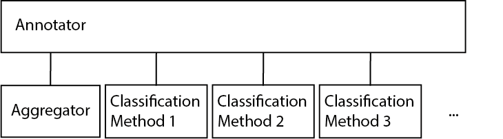
We implemented the Annotator Class which lets a user create new categories of sequences. Each instance of the Annotator Class is responsible for one category. As depicted in Figure 6 each Annotator is linked to an Aggregator and one or more Classification Methods (see Sections A.4 and A.5 below). The Annotator is responsible for running all its Classification Methods for each sequence, providing the Aggregator with results and storing the 5-Level membership results for future use.
A.4 Aggregator
An Aggregator, as the name suggests, aggregates the results from the Classification Methods and returns a 5-Level membership value.
A.5 Classification Methods
Classification Methods are functions which take all the information about a sequence (i.e. all the fields described in Section A) as an input and return results of some test which are then further processed by the Aggregator.
Note, all Classification Methods have to check whether the fields which have to be accessed by the test do exist for the given sequence, i.e. the field is not empty or NULL.
As we will see in the following subsections, a Classification Method can be something as simple as searching for a given word in the name of the sequence or more complex like doing some advanced calculations based on the value. However, Classification Methods should be designed to have a rather short runtime per sequence since the same function has to run on all sequences in the dataset. As a rule of thumb, when a test takes one second per sequence the total runtime on the current dataset will be about 4 days.
Mathematical
We used Mathematical Tests to check for properties of the values of the sequences. These methods bear some limitations one needs to be aware off. Some tests require a minimal number of values to return meaningful results. For example a sequence with only given values is not suitable for fitting a polynomial of degree to it. On the other hand if the sequence truly would have a polynomial form then elements would be easy to calculate and there would probably be more values provided. Following are descriptions of the mathematical Classification Methods we used.
- •
Newton’s Divided Difference We used Newton’s Divided Difference Method to calculate the degree a polynomial would have to have in order to fit to the values of the sequence. Intuitively this is the discrete signal analog of repeatedly taking the derivative of a polynomial until we end up with the constant function. By counting the number of iterations, we get the degree a fitting polynomial would need to have, which we can then use for Polynomial Interpolation.
- •
Polynomial Interpolation
We used the SymPy[43] library to perform symbolic polynomial interpolation with the degree calculated by Newton’s Divided Difference Method. This allows us to fit a polynomial of degree to the first values of the sequence and use the remaining values to calculate the error between the fitted polynomial and the actual values. Of course we need to assert that there are enough values, which were not used during interpolation, to be able to calculate a meaningful error. In cases where the error between the fitted polynomial and the actual values is and we have enough values, we conclude that the sequence in question indeed has a polynomial form.
- •
Exponentials
To detect exponential sequences, such as , Powers of 3, or , , directly from their values we first calculate the sequence of quotients . Each element of is the quotient of two subsequent elements of the original sequence:
(1) Purely exponential sequences, like Powers of 3, produce a constant-valued . In our example for all . Such sequences pass this test immediately.
Sequences that are dominated by an exponential like , , produce a sequence of quotient that approaches a constant value. In this example we get
(2) We approximate the limit of by checking the very last values of it that can be calculated from the given data. If the last elements are all within some threshold range of the final value we conclude that the sequence probably is dominated by an exponential function.
- •
Primality
Using SymPy again, we tested which sequences can be interpreted as the application of the above classes of functions to prime numbers. The way we implemented this test was limited to numbers smaller than (or about ).
- •
Boundedness
Testing the absolute values of the sequence elements for boundedness by different values, is an easy but insightful series of tests.
- •
Palindrome
This test checks whether all elements in a sequence are palindromic, i.e. if all values are numbers that are the same when read from left to right as well as from right to left. Trivially this is true for all sequences that contain only values smaller than since all single-digit numbers are palindromic (i.e. is the same number when read from either direction). The results from this test depend on the base of the number system used to display the values of the sequence. For example is palindromic in base but in base it is not: .
- •
Periodicity
We tested whether a sequence has a repeating part up to a maximal period length of elements. To pass the test a sequence needs to have at least full periods in the value_list.
String Search
Since most of the fields in the dataset are populated by plain text, one of the easiest methods to get information about a sequence is the search for specific words or strings within a given fields. This method can be a reliable indicator whether a sequence does belong to a category, for example performing a string search of the word prime on the name of , Smallest prime larger than , can serve as a good indicator that indeed is at least in some way related to prime numbers. However, the opposite conclusion is harder to draw, is a sequence truly unrelated to prime numbers just because it is not mentioned in the name or comments?
Regular Expressions
Regular Expressions served as a powerful tool to check for patterns in the data. For example we created the regular expression
    a\(n\)=[0-9]*\*?a\(n[\+\-][0-9]+\)[\+\-][0-9]*\*?
    a\(n[\+\-][0-9]+\)([\+\-][0-9]*\*?a\(n[\+\-][0-9]+\))*
Which matches character patterns like
| (3) |
Due to the similarity with the well known Fibonacci Sequence (), we call sequences with formulas that are matched by above regular expression Fibonacci-Like.
Appendix B Synthetic Generation
In this section we explain the steps followed to create synthetic sequences.
From the identified categories (cf. fig. 2) in the OEIS database, we have elected a significant and representative subset and augmented their organic entries with synthetic data. For each category, a total of 500K synthetic sequences have been generated. The sequences were generated with logaritmically increasing length of the generating formula. This way, most of the sequences-generating expressions are relatively short (motivated by Kolmogorov complexity, cf. Section 2), but longer sequences remain playing a significant role in the dataset. In the following, we provide information how synthetic extensions of each sequence category are created using context-free grammars. Typically, the “logical” terminals in our grammars are and the non-terminals . is defined as the non-terminal which represents the number constants with multiple digits. The reason why we consider it a non-terminal is that we count the length of polynomial based on the number of non-terminals only.
Polynomial
The context-free grammar for polynomials is defined as:
Exponential
Context-free grammar of exponentials group is defined as:
Prime
In this group, we introduce a non terminal , which evaluated at value returns the prime number. That is, , , , and so on. This way we inject in our sequences prior knowledge about prime numbers. More concretely, the context free grammar is defined as:
Periodic
Periodic group makes use of the previous grammars, but it also has a non terminal that is added in the root of the grammar, which makes the whole sequence repeat only the first few numbers. More concretely, we can phrase this as a grammar too, by adding primitive as a root of the grammar
Let sequence be any sequence, then the function is defined as .
Modulo
In this group we add a non terminal modulo and we define the grammar as:
Trigonometric
Here we add two non terminals and . The grammar defined in this group can be found in the following.
Finite
Finite is a simple group where we only create a list of finite numbers. They are created the same way by using previous rules but they are cut at a specific place randomly.
Increasing
The next three groups are meta-categories, for which no specific grammar is used, but the property is inferred afterwards. If the sequence generated is monotonically increasing, then it is labelled as increasing.
Bounded
If the sequence is bounded by a number, then it is labelled as bounded. For example is bounded.
Unique
If all numbers in the sequence are distinct, then it is marked as unique. We generate at least first 500 numbers of the sequence to check this property. Of course, this may not be the case for the numbers appearing later in the sequence.
B.1 Hosting and Maintenance of the Dataset
The dataset is available through the ETH Research Collection and is directly accessible with DOI 10.3929/ethz-b-000562705 [5]. The ETH Research Collection guarantees minimal data retention period of 10 years. The presence of the dataset will be maintained by the D-ITET DISCO and ISG groups. Members of DISCO will also be responsible for the maintenance of the dataset in response to queries or any errors found and reported – please email fact@ethz.ch to do so.
Appendix C Baseline Models
To provide baselines for model performance on the above tasks, we use a total of 24 different models across our bench-marking tasks, namely 4 neural models, 9 classical classifiers, and 11 standard regressors. The following sections describe the architecture of these models. For consistency, we used the random seed wherever it could be specified.
C.1 Neural Models
C.1.1 Dense Neural Network
The densely connected neural network is composed of three hidden layers with 64, 32 and 16 neurons each, and an input layer with 50 neurons, corresponding to the first 50 integers of the sequence.
Each hidden neuron is activated with the rectified function (ReLU).
The last layer is activated with the sigmoid function in case of classification tasks, and linearly activated in case of regression.
In multi-class-classification, 10 output neurons with sigmoid activation (one for each main class) are used.
In terms of hyperparemeter-tuning, we focused on the depth layout and kernel regularisations.
Our grid search contained the following discrete ranges for each parameter:
C.1.2 Recurrent Neural Network
The architecture of our recurrent model consists of three Long Short-Term Memory [15] layers, each with 64, 32 and 16 units respectively. The first two layers produce the whole sequence, whereas the last layer only yields the last output. The units of the last layer are fed into a dense-layer with a sigmoidal or linear activation. No dropout was used for RNNs. The hyperparameter-grid-search included:
C.1.3 Convolutional Neural Network
Here we used a simple stack containing a convolutional layer with kernel size 2, 10 filters and a pooling-layer of size 2, with unit strides. The network was composed of three of these stacks, terminating in a dense layer with the same activation as above. The hyperparameter-tuning focused on filter and kernel size:
C.1.4 Transformer
We followed the transformer architecture of [44] with only the normalisation layers excluded. We use six transformer blocks for the encoder and three for the decoder decoder. Each multi-headed attention unit consists of 20 attention heads and the output dimension of the embedding and feed-forward layers is 12. We focused on the number of attention heads as well as the embedding dimension in our grid search: .
C.2 Standard Classifiers and Regressors
Table 4 summarizes all standard classifiers and regressors we used. Each standard model is implemented with the scikit-learn [27] library for python. For each model we used its standard parameters. Classification performance is measured in binary-accuracy whereas multiclass performance across all categories is measured with macro-averaged F1-score.
| Classifiers | Regressors | ||
|---|---|---|---|
| KNNC | k-Nearest Neighbors | KNNR | k-Nearest Neighbors |
| GNBC | Gaussian naive Bayes | LIR | Linear Regressor |
| LSVC | Linear Sup. Vector Machine | RIR | Ridge Regressor |
| DTC | Decision Tree | LAR | Lasso Regressor |
| RFC | Random Forest | ENR | Elastic Net |
| GBC | Gradient Boosting | DTR | Decision Tree |
| ABC | AdaBoost | RFR | Random Forest |
| XGBC | XG Boost | GBR | Gradient Boosting |
| DYC | Dummy Classifier | ABR | AdaBoost |
| XGBR | XGBoost | ||
| DYR | Dummy Regressor | ||
| Max # of Epochs | 20 |
| Optimizer | Adam |
| DNN L1 regularizer | 0.001 |
| DNN L2 regularizer | 0.0001 |
| RNN L1 regularizer | 0.001 |
| RNN L2 regularizer | 0.0001 |
| RNN dropout probability | 0 |
| CNN filter count | 10 |
| margin distance | 1 |
C.3 Loss and Metrics
C.3.1 Binary-Crossentropy
For our tasks in static mode we used binary-crossentropy as a loss for classification and mean squared logarithmic error for regression.
C.3.2 Flexible Contrastive Loss
In dynamic mode we went for a contrastive loss described in the following formula:
| (4) |
where is the euclidean distance between two sequences in the embedding space and is the margin-distance which penalises dissimilar pairs only if their distance is inside its radius. The goal of this loss is to embed similar sequences near each other in terms of the euclidean distance and different ones further away. The parameter functions as a measurement of similarity. In each dynamic task we define this measurement differently. In sequence similarity, is the indicator function between two classes. In sequence continuation, is the fraction between the first similar numbers of two sequences and its total length, whereas in sequence unmasking is the fraction of masked entries in a sequence paired with its unmasked counterpart. With this approach we seek to build an embedding space that learns to differentiate different sequences according to our tasks given.
C.4 Hosting and Maintenance of the Benchmarking Baseline Models
The bechmarking baseline models are available through the ETH Research Collection and are directly accessible through DOI 10.3929/ethz-b-000565644 [4]. The ETH Research Collection guarantees minimal data retention period of 10 years. The presence of the models will be maintained by the D-ITET DISCO and ISG groups. Members of DISCO will also be responsible for the maintenance of the models in response to queries or any errors found and reported – please email fact@ethz.ch to do so.
Appendix D Baseline Model Performance
| Model | Dataset | Scope | ||||||||||
|---|---|---|---|---|---|---|---|---|---|---|---|---|
| Within | Across | |||||||||||
| polynomial | exponential | trigonometric | periodic | finite | modulo | prime | bounded | increasing | unique | all classes | ||
| Sequence | [binary-accuracy] | [f1-score] | ||||||||||
| Classification | ||||||||||||
| DNN | oeis | 0.634 | 0.575 | 0.621 | 0.451 | n.a. | 0.458 | 0.545 | 0.815 | 0.666 | 0.776 | 0.330 |
| synth | 0.784 | 0.754 | 0.815 | 0.746 | 0.748 | 0.801 | 0.876 | 0.990 | 0.857 | 0.959 | 0.430 | |
| RNN | oeis | 0.588 | 0.712 | 0.456 | 0.474 | n.a. | 0.489 | 0.586 | 0.860 | 0.840 | 0.834 | 0.370 |
| synth | 0.790 | 0.788 | 0.828 | 0.764 | 0.755 | 0.825 | 0.907 | 0.998 | 0.954 | 0.976 | 0.530 | |
| CNN | oeis | 0.569 | 0.550 | 0.619 | 0.470 | n.a. | 0.483 | 0.514 | 0.800 | 0.575 | 0.694 | 0.220 |
| synth | 0.769 | 0.704 | 0.792 | 0.727 | 0.736 | 0.769 | 0.843 | 0.976 | 0.752 | 0.793 | 0.390 | |
| Transformer | oeis | 0.599 | 0.672 | 0.524 | 0.464 | n.a. | 0.475 | 0.578 | 0.825 | 0.661 | 0.793 | 0.330 |
| synth | 0.791 | 0.763 | 0.817 | 0.759 | 0.753 | 0.814 | 0.883 | 0.993 | 0.882 | 0.905 | 0.440 | |
| KNNC | oeis | 0.650 | 0.615 | 0.545 | 0.489 | n.a. | 0.484 | 0.559 | 0.793 | 0.693 | 0.756 | 0.330 |
| synth | 0.760 | 0.765 | 0.797 | 0.707 | 0.713 | 0.810 | 0.896 | 0.994 | 0.883 | 0.890 | 0.410 | |
| GNBC | oeis | 0.626 | 0.276 | 0.560 | 0.464 | n.a. | 0.474 | 0.476 | 0.810 | 0.683 | 0.667 | 0.230 |
| synth | 0.769 | 0.646 | 0.764 | 0.721 | 0.732 | 0.736 | 0.635 | 0.916 | 0.634 | 0.648 | 0.370 | |
| LSVC | oeis | 0.709 | 0.377 | 0.646 | 0.410 | n.a. | 0.485 | 0.508 | 0.763 | 0.546 | 0.637 | 0.310 |
| synth | 0.759 | 0.622 | 0.771 | 0.717 | 0.680 | 0.745 | 0.819 | 0.954 | 0.586 | 0.718 | 0.350 | |
| DTC | oeis | 0.618 | 0.607 | 0.497 | 0.480 | n.a. | 0.483 | 0.558 | 0.820 | 0.624 | 0.727 | 0.360 |
| synth | 0.722 | 0.754 | 0.807 | 0.690 | 0.677 | 0.812 | 0.887 | 0.995 | 0.918 | 0.949 | 0.490 | |
| RFC | oeis | 0.595 | 0.680 | 0.507 | 0.493 | n.a. | 0.468 | 0.563 | 0.843 | 0.579 | 0.787 | 0.340 |
| synth | 0.789 | 0.791 | 0.837 | 0.759 | 0.749 | 0.830 | 0.908 | 0.998 | 0.938 | 0.963 | 0.510 | |
| GBC | oeis | 0.576 | 0.495 | 0.643 | 0.478 | n.a. | 0.470 | 0.548 | 0.821 | 0.623 | 0.788 | 0.270 |
| synth | 0.785 | 0.746 | 0.804 | 0.758 | 0.751 | 0.803 | 0.872 | 0.990 | 0.835 | 0.860 | 0.400 | |
| ABC | oeis | 0.617 | 0.392 | 0.658 | 0.470 | n.a. | 0.457 | 0.497 | 0.782 | 0.511 | 0.691 | 0.310 |
| synth | 0.773 | 0.676 | 0.777 | 0.741 | 0.737 | 0.761 | 0.829 | 0.958 | 0.669 | 0.766 | 0.380 | |
| XGBC | oeis | 0.603 | 0.670 | 0.499 | 0.480 | n.a. | 0.477 | 0.595 | 0.842 | 0.674 | 0.813 | 0.370 |
| synth | 0.789 | 0.782 | 0.828 | 0.762 | 0.754 | 0.827 | 0.901 | 0.997 | 0.915 | 0.962 | 0.510 | |
| DYC | oeis | 0.500 | 0.500 | 0.500 | 0.500 | n.a. | 0.500 | 0.500 | 0.500 | 0.500 | 0.500 | 0.500 |
| synth | 0.500 | 0.500 | 0.500 | 0.500 | 0.500 | 0.500 | 0.500 | 0.500 | 0.500 | 0.500 | 0.500 | |
| Next Sequence-Part | [binary-accuracy] | |||||||||||
| Prediction | ||||||||||||
| DNN | oeis | 0.658 | 0.664 | 0.719 | 0.778 | n.a. | 0.760 | 0.744 | 0.749 | 0.753 | 0.726 | 0.733 |
| synth | 0.941 | 0.927 | 0.940 | 0.943 | 0.939 | 0.918 | 0.914 | 0.943 | 0.924 | 0.936 | 0.943 | |
| RNN | oeis | 0.869 | 0.890 | 0.827 | 0.849 | n.a. | 0.855 | 0.860 | 0.833 | 0.876 | 0.889 | 0.869 |
| synth | 0.988 | 0.973 | 0.979 | 0.987 | 0.988 | 0.972 | 0.955 | 0.978 | 0.982 | 0.976 | 0.984 | |
| CNN | oeis | 0.526 | 0.520 | 0.540 | 0.566 | n.a. | 0.548 | 0.535 | 0.566 | 0.547 | 0.539 | 0.551 |
| synth | 0.893 | 0.912 | 0.922 | 0.903 | 0.895 | 0.898 | 0.890 | 0.915 | 0.885 | 0.901 | 0.900 | |
| Transformer | oeis | 0.690 | 0.666 | 0.707 | 0.792 | n.a. | 0.759 | 0.747 | 0.752 | 0.744 | 0.737 | 0.736 |
| synth | 0.947 | 0.930 | 0.945 | 0.947 | 0.949 | 0.927 | 0.919 | 0.946 | 0.926 | 0.943 | 0.938 | |
| Model | Dataset | Metric | Scope | |||||||||
| Within | ||||||||||||
| polynomial | exponential | trigonometric | periodic | finite | modulo | prime | bounded | increasing | unique | |||
| Sequence | [binary-accuracy] | |||||||||||
| Similarity | ||||||||||||
| DNN | oeis | Top-1 | 0.20 | 0.00 | 0.08 | 0.16 | n.a. | 0.09 | 0.12 | 0.07 | 0.09 | 0.08 |
| Top-3 | 0.23 | 0.00 | 0.19 | 0.16 | n.a. | 0.23 | 0.21 | 0.29 | 0.32 | 0.26 | ||
| Top-5 | 0.44 | 0.00 | 0.27 | 0.33 | n.a. | 0.30 | 0.34 | 0.43 | 0.45 | 0.48 | ||
| synth | Top-1 | 0.12 | 0.13 | 0.19 | 0.10 | 0.09 | 0.11 | 0.32 | 0.10 | 0.07 | 0.09 | |
| Top-3 | 0.27 | 0.34 | 0.30 | 0.25 | 0.31 | 0.23 | 0.54 | 0.38 | 0.27 | 0.33 | ||
| Top-5 | 0.43 | 0.46 | 0.44 | 0.44 | 0.40 | 0.57 | 0.69 | 0.57 | 0.44 | 0.48 | ||
| RNN | oeis | Top-1 | 0.07 | 0.00 | 0.04 | 0.20 | n.a. | 0.13 | 0.14 | 0.06 | 0.06 | 0.11 |
| Top-3 | 0.25 | 0.00 | 0.27 | 0.50 | n.a. | 0.35 | 0.16 | 0.34 | 0.31 | 0.25 | ||
| Top-5 | 0.53 | 0.00 | 0.40 | 0.50 | n.a. | 0.41 | 0.34 | 0.45 | 0.44 | 0.42 | ||
| synth | Top-1 | 0.17 | 0.11 | 0.20 | 0.08 | 0.10 | 0.13 | 0.35 | 0.12 | 0.07 | 0.08 | |
| Top-3 | 0.32 | 0.29 | 0.39 | 0.32 | 0.32 | 0.25 | 0.56 | 0.40 | 0.29 | 0.32 | ||
| Top-5 | 0.41 | 0.38 | 0.47 | 0.42 | 0.47 | 0.49 | 0.70 | 0.56 | 0.41 | 0.51 | ||
| CNN | oeis | Top-1 | 0.15 | 0.00 | 0.06 | 0.00 | n.a. | 0.06 | 0.16 | 0.14 | 0.07 | 0.15 |
| Top-3 | 0.34 | 0.12 | 0.31 | 0.00 | n.a. | 0.38 | 0.32 | 0.43 | 0.26 | 0.36 | ||
| Top-5 | 0.34 | 0.75 | 0.41 | 0.40 | n.a. | 0.47 | 0.46 | 0.59 | 0.39 | 0.50 | ||
| synth | Top-1 | 0.09 | 0.14 | 0.16 | 0.07 | 0.13 | 0.11 | 0.32 | 0.17 | 0.08 | 0.10 | |
| Top-3 | 0.37 | 0.39 | 0.37 | 0.42 | 0.29 | 0.32 | 0.61 | 0.49 | 0.30 | 0.39 | ||
| Top-5 | 0.50 | 0.41 | 0.60 | 0.48 | 0.47 | 0.51 | 0.66 | 0.64 | 0.44 | 0.60 | ||
| Transformer | oeis | Top-1 | 0.03 | 0.00 | 0.13 | 0.00 | n.a. | 0.05 | 0.18 | 0.11 | 0.09 | 0.09 |
| Top-3 | 0.31 | 0.00 | 0.39 | 0.10 | n.a. | 0.33 | 0.28 | 0.42 | 0.29 | 0.38 | ||
| Top-5 | 0.48 | 0.66 | 0.43 | 0.20 | n.a. | 0.49 | 0.40 | 0.50 | 0.43 | 0.55 | ||
| synth | Top-1 | 0.21 | 0.13 | 0.31 | 0.12 | 0.17 | 0.10 | 0.36 | 0.13 | 0.07 | 0.10 | |
| Top-3 | 0.44 | 0.32 | 0.41 | 0.41 | 0.37 | 0.32 | 0.56 | 0.50 | 0.32 | 0.35 | ||
| Top-5 | 0.67 | 0.52 | 0.63 | 0.51 | 0.52 | 0.55 | 0.65 | 0.61 | 0.44 | 0.58 | ||
| Model | Dataset | Scope | ||||||||||
|---|---|---|---|---|---|---|---|---|---|---|---|---|
| Within | Across | |||||||||||
| polynomial | exponential | trigonometric | periodic | finite | modulo | prime | bounded | increasing | unique | all classes | ||
| Sequence | [root-mean-squared-log-error] | |||||||||||
| Continuation | ||||||||||||
| DNN | oeis | 0.750 | 0.700 | 0.588 | 0.576 | n.a. | 0.567 | 0.617 | 0.519 | 0.600 | 0.614 | 0.597 |
| synth | 0.496 | 0.408 | 0.345 | 0.485 | 0.489 | 0.398 | 0.379 | 0.372 | 0.477 | 0.452 | 0.430 | |
| RNN | oeis | 0.738 | 0.692 | 0.561 | 0.561 | n.a. | 0.554 | 0.602 | 0.506 | 0.577 | 0.614 | 0.603 |
| synth | 0.470 | 0.375 | 0.317 | 0.466 | 0.461 | 0.381 | 0.345 | 0.351 | 0.457 | 0.424 | 0.406 | |
| CNN | oeis | 0.776 | 0.768 | 0.765 | 0.679 | n.a. | 0.727 | 0.758 | 0.686 | 0.730 | 0.737 | 0.733 |
| synth | 0.586 | 0.550 | 0.498 | 0.585 | 0.581 | 0.557 | 0.623 | 0.536 | 0.599 | 0.612 | 0.579 | |
| Transformer | oeis | 1.632 | 1.596 | 0.573 | 1.113 | n.a. | 0.545 | 0.573 | 0.503 | 0.575 | 0.593 | 0.578 |
| synth | 2.051 | 1.420 | 0.308 | 1.978 | 0.452 | 0.365 | 0.335 | 0.341 | 0.449 | 0.415 | 0.395 | |
| KNNR | oeis | 0.955 | 0.874 | 0.761 | 0.807 | n.a. | 0.730 | 0.796 | 0.669 | 0.783 | 0.832 | 0.808 |
| synth | 0.575 | 0.451 | 0.373 | 0.560 | 0.551 | 0.459 | 0.401 | 0.433 | 0.564 | 0.513 | 0.486 | |
| LIR | oeis | 0.872 | 0.784 | 0.723 | 0.880 | n.a. | 0.710 | 0.846 | 0.704 | 0.786 | 0.821 | 0.797 |
| synth | 0.694 | 0.633 | 0.545 | 0.696 | 0.692 | 0.611 | 0.770 | 0.613 | 0.701 | 0.724 | 0.682 | |
| RIR | oeis | 0.873 | 0.784 | 0.721 | 0.875 | n.a. | 0.713 | 0.846 | 0.703 | 0.786 | 0.822 | 0.797 |
| synth | 0.692 | 0.632 | 0.546 | 0.695 | 0.692 | 0.613 | 0.769 | 0.613 | 0.701 | 0.725 | 0.682 | |
| LAR | oeis | 0.910 | 0.750 | 0.727 | 1.012 | n.a. | 0.734 | 0.882 | 0.743 | 0.798 | 0.856 | 0.827 |
| synth | 0.750 | 0.703 | 0.615 | 0.754 | 0.748 | 0.688 | 0.812 | 0.683 | 0.765 | 0.783 | 0.747 | |
| ENR | oeis | 0.886 | 0.756 | 0.722 | 0.951 | n.a. | 0.723 | 0.862 | 0.724 | 0.793 | 0.840 | 0.814 |
| synth | 0.722 | 0.672 | 0.583 | 0.727 | 0.723 | 0.656 | 0.794 | 0.651 | 0.734 | 0.754 | 0.716 | |
| DTR | oeis | 0.868 | 0.801 | 0.693 | 0.741 | n.a. | 0.663 | 0.731 | 0.618 | 0.695 | 0.749 | 0.730 |
| synth | 0.496 | 0.392 | 0.328 | 0.492 | 0.487 | 0.391 | 0.351 | 0.368 | 0.490 | 0.445 | 0.427 | |
| RFR | oeis | 0.871 | 0.797 | 0.696 | 0.740 | n.a. | 0.666 | 0.730 | 0.619 | 0.696 | 0.748 | 0.730 |
| synth | 0.496 | 0.393 | 0.325 | 0.492 | 0.488 | 0.396 | 0.348 | 0.368 | 0.491 | 0.446 | 0.427 | |
| GBR | oeis | 0.857 | 0.789 | 0.622 | 0.694 | n.a. | 0.650 | 0.706 | 0.578 | 0.694 | 0.726 | 0.702 |
| synth | 0.544 | 0.459 | 0.377 | 0.540 | 0.535 | 0.446 | 0.420 | 0.420 | 0.545 | 0.510 | 0.484 | |
| ABR | oeis | 0.907 | 0.868 | 0.782 | 0.894 | n.a. | 0.754 | 0.837 | 0.776 | 0.796 | 0.878 | 0.842 |
| synth | 0.635 | 0.621 | 0.542 | 0.667 | 0.659 | 0.594 | 0.652 | 0.635 | 0.658 | 0.672 | 0.662 | |
| XGBR | oeis | 0.869 | 0.796 | 0.679 | 0.726 | n.a. | 0.651 | 0.707 | 0.607 | 0.688 | 0.735 | 0.719 |
| synth | 0.499 | 0.400 | 0.330 | 0.497 | 0.490 | 0.400 | 0.360 | 0.372 | 0.496 | 0.452 | 0.433 | |
| DYR | oeis | 0.972 | 0.770 | 0.821 | 1.202 | n.a. | 0.788 | 0.912 | 0.883 | 0.860 | 0.930 | 0.923 |
| synth | 0.832 | 0.868 | 0.807 | 0.847 | 0.844 | 0.858 | 0.877 | 0.866 | 0.876 | 0.871 | 0.877 | |
| Model | Dataset | Metric | Scope | ||||||||||
| Within | Across | ||||||||||||
| polynomial | exponential | trigonometric | periodic | finite | modulo | prime | bounded | increasing | unique | all classes | |||
| Sequence | [top-k-root-mean-squared-error] | ||||||||||||
| Similarity | |||||||||||||
| DNN | oeis | Top-1 | 2.037 | 1.662 | 3.542 | 1.392 | n.a. | 1.867 | 1.432 | 0.850 | 2.488 | 1.300 | 2.668 |
| Top-3 | 0.931 | 1.662 | 0.442 | 0.390 | n.a. | 0.785 | 0.587 | 0.367 | 0.900 | 0.912 | 0.599 | ||
| Top-5 | 0.855 | 1.662 | 0.361 | 0.152 | n.a. | 0.696 | 0.433 | 0.250 | 0.561 | 0.912 | 0.301 | ||
| synth | Top-1 | 5.847 | 3.261 | 5.616 | 2.790 | 2.695 | 1.597 | 1.896 | 3.951 | 2.153 | 2.302 | 2.144 | |
| Top-3 | 0.870 | 0.927 | 0.365 | 1.192 | 1.483 | 0.475 | 1.246 | 0.534 | 1.130 | 1.900 | 1.690 | ||
| Top-5 | 0.752 | 0.549 | 0.365 | 0.766 | 1.483 | 0.448 | 0.944 | 0.534 | 0.825 | 0.520 | 1.690 | ||
| RNN | oeis | Top-1 | 2.089 | 2.278 | 1.624 | 1.735 | n.a. | 1.326 | 1.831 | 1.264 | 1.473 | 1.450 | 1.367 |
| Top-3 | 1.038 | 1.025 | 0.677 | 0.661 | n.a. | 0.645 | 0.823 | 0.597 | 0.617 | 0.658 | 0.596 | ||
| Top-5 | 0.706 | 0.665 | 0.429 | 0.439 | n.a. | 0.435 | 0.585 | 0.406 | 0.427 | 0.457 | 0.383 | ||
| synth | Top-1 | 1.889 | 1.488 | 0.974 | 2.193 | 2.331 | 1.034 | 1.210 | 1.290 | 1.453 | 1.604 | 1.509 | |
| Top-3 | 0.784 | 0.566 | 0.405 | 0.954 | 1.033 | 0.448 | 0.508 | 0.589 | 0.654 | 0.713 | 0.667 | ||
| Top-5 | 0.506 | 0.364 | 0.244 | 0.595 | 0.607 | 0.290 | 0.320 | 0.355 | 0.401 | 0.476 | 0.438 | ||
| CNN | oeis | Top-1 | 3.117 | 2.943 | 1.957 | 1.715 | n.a. | 2.426 | 1.570 | 1.430 | 1.950 | 1.490 | 1.825 |
| Top-3 | 1.309 | 1.302 | 0.679 | 0.813 | n.a. | 1.046 | 0.702 | 0.501 | 0.579 | 1.003 | 0.807 | ||
| Top-5 | 0.631 | 0.646 | 0.585 | 0.521 | n.a. | 0.736 | 0.361 | 0.296 | 0.406 | 0.711 | 0.428 | ||
| synth | Top-1 | 2.475 | 1.662 | 1.399 | 3.533 | 2.338 | 1.848 | 7.013 | 2.288 | 2.333 | 2.033 | 2.348 | |
| Top-3 | 1.060 | 0.695 | 1.115 | 1.031 | 1.151 | 0.880 | 1.007 | 1.152 | 0.826 | 0.871 | 1.105 | ||
| Top-5 | 0.664 | 0.440 | 0.836 | 0.777 | 0.697 | 0.647 | 0.648 | 0.682 | 0.463 | 0.613 | 0.643 | ||
| Transformer | oeis | Top-1 | 1.503 | 1.408 | 0.984 | 0.786 | n.a. | 0.977 | 1.161 | 0.663 | 1.022 | 0.935 | 0.847 |
| Top-3 | 0.746 | 0.748 | 0.398 | 0.382 | n.a. | 0.454 | 0.584 | 0.348 | 0.499 | 0.438 | 0.383 | ||
| Top-5 | 0.529 | 0.524 | 0.253 | 0.287 | n.a. | 0.285 | 0.414 | 0.284 | 0.376 | 0.288 | 0.267 | ||
| synth | Top-1 | 1.816 | 0.962 | 0.788 | 1.730 | 1.651 | 0.811 | 0.801 | 0.873 | 1.084 | 1.198 | 1.258 | |
| Top-3 | 0.727 | 0.410 | 0.312 | 0.787 | 0.706 | 0.316 | 0.331 | 0.389 | 0.447 | 0.507 | 0.490 | ||
| Top-5 | 0.448 | 0.248 | 0.202 | 0.484 | 0.418 | 0.225 | 0.205 | 0.233 | 0.270 | 0.331 | 0.284 | ||
| Sequence | [top-k-root-mean-squared-error] | ||||||||||||
| Unmasking | |||||||||||||
| DNN | oeis | Top-1 | 3.702 | 3.529 | 3.460 | 3.248 | n.a. | 3.451 | 3.451 | 3.274 | 3.307 | 3.315 | 3.384 |
| Top-3 | 3.305 | 3.163 | 2.936 | 2.917 | n.a. | 3.114 | 3.059 | 2.976 | 3.061 | 3.027 | 3.061 | ||
| Top-5 | 3.125 | 3.000 | 2.748 | 2.779 | n.a. | 2.972 | 2.880 | 2.878 | 2.925 | 2.903 | 2.918 | ||
| synth | Top-1 | 4.240 | 3.711 | 3.374 | 4.062 | 4.092 | 3.633 | 3.786 | 3.619 | 3.839 | 3.766 | 3.855 | |
| Top-3 | 3.898 | 3.448 | 2.958 | 3.710 | 3.744 | 3.353 | 3.321 | 3.356 | 3.547 | 3.470 | 3.524 | ||
| Top-5 | 3.776 | 3.335 | 2.825 | 3.582 | 3.593 | 3.239 | 3.161 | 3.236 | 3.441 | 3.361 | 3.408 | ||
| RNN | oeis | Top-1 | 3.789 | 3.720 | 3.548 | 3.314 | n.a. | 3.484 | 3.499 | 3.320 | 3.490 | 3.485 | 3.455 |
| Top-3 | 3.206 | 3.175 | 3.052 | 2.876 | n.a. | 3.060 | 2.998 | 2.908 | 3.109 | 3.083 | 3.091 | ||
| Top-5 | 3.010 | 2.990 | 2.847 | 2.688 | n.a. | 2.898 | 2.830 | 2.757 | 2.925 | 2.909 | 2.944 | ||
| synth | Top-1 | 4.141 | 3.765 | 3.368 | 4.094 | 4.115 | 3.535 | 3.775 | 3.696 | 3.674 | 3.913 | 3.855 | |
| Top-3 | 3.663 | 3.463 | 3.082 | 3.639 | 3.663 | 3.254 | 3.314 | 3.346 | 3.328 | 3.515 | 3.511 | ||
| Top-5 | 3.473 | 3.291 | 2.961 | 3.472 | 3.507 | 3.140 | 3.162 | 3.197 | 3.208 | 3.370 | 3.379 | ||
| CNN | oeis | Top-1 | 3.738 | 3.699 | 3.615 | 3.268 | n.a. | 3.383 | 3.521 | 3.165 | 3.453 | 3.257 | 3.355 |
| Top-3 | 2.943 | 2.922 | 2.873 | 2.594 | n.a. | 2.683 | 2.785 | 2.510 | 2.727 | 2.643 | 2.690 | ||
| Top-5 | 2.689 | 2.631 | 2.577 | 2.370 | n.a. | 2.437 | 2.539 | 2.260 | 2.490 | 2.423 | 2.440 | ||
| synth | Top-1 | 3.906 | 3.584 | 3.223 | 3.791 | 3.886 | 3.500 | 3.646 | 3.531 | 3.627 | 3.702 | 3.611 | |
| Top-3 | 3.179 | 3.100 | 2.811 | 3.128 | 3.168 | 2.968 | 3.112 | 3.008 | 2.988 | 3.122 | 3.033 | ||
| Top-5 | 2.931 | 2.799 | 2.642 | 2.891 | 2.898 | 2.784 | 2.890 | 2.834 | 2.747 | 2.899 | 2.812 | ||
| Transformer | oeis | Top-1 | 3.635 | 3.674 | 3.586 | 3.245 | n.a. | 3.465 | 3.556 | 3.378 | 3.456 | 3.606 | 3.524 |
| Top-3 | 3.042 | 3.045 | 2.951 | 2.798 | n.a. | 2.991 | 2.974 | 2.903 | 2.947 | 3.038 | 3.017 | ||
| Top-5 | 2.820 | 2.781 | 2.658 | 2.606 | n.a. | 2.808 | 2.717 | 2.717 | 2.756 | 2.816 | 2.811 | ||
| synth | Top-1 | 3.953 | 3.719 | 3.403 | 3.968 | 4.079 | 3.478 | 3.638 | 3.605 | 3.717 | 3.780 | 3.757 | |
| Top-3 | 3.374 | 3.259 | 3.019 | 3.395 | 3.475 | 3.190 | 3.115 | 3.226 | 3.293 | 3.359 | 3.291 | ||
| Top-5 | 3.171 | 3.067 | 2.872 | 3.161 | 3.259 | 3.041 | 2.941 | 3.045 | 3.121 | 3.173 | 3.091 | ||
D.1 Compute Time Breakdown
| Model | Task | ||||
|---|---|---|---|---|---|
| classification | next part pred. | continuation | similarity | unmasking | |
| mean task training and evaluation time in minutes | |||||
| DNN | 23 | 214 | 98 | 32 | 168 |
| RNN | 44 | 428 | 234 | 57 | 345 |
| CNN | 35 | 388 | 198 | 48 | 246 |
| Transformer | 48 | 465 | 256 | 45 | 326 |
| KNNC | 67 | - | - | - | - |
| GNBC | 7 | - | - | - | - |
| DTC | 14 | - | - | - | - |
| XGBC | 17 | - | - | - | - |
| LSVC | 26 | - | - | - | - |
| RFC | 14 | - | - | - | - |
| GBC | 9 | - | - | - | - |
| ABC | 23 | - | - | - | - |
| XGBC | 11 | - | - | - | - |
| KNNR | - | - | - | 72 | - |
| RIR | - | - | - | 42 | - |
| LIR | - | - | - | 37 | - |
| ENR | - | - | - | 61 | - |
| LAR | - | - | - | 58 | - |
| DTR | - | - | - | 50 | - |
| ABR | - | - | - | 24 | - |
| GBR | - | - | - | 27 | - |
| DYR | - | - | - | 36 | - |
| XGBR | - | - | - | 22 | - |
| RFR | - | - | - | 28 | - |
| LSVR | - | - | - | 41 | - |
Appendix E Expectations on Model Performance
We believe that our the baseline classifier performance can be vastly improved on and shifted towards the region of to . We would expect tailored models to have near-perfect performance on the next part prediction task, RMSLEs of below (corresponding to uniform sequence element logarithm difference) in the continuation task, and top--RMSEs in the similarity and unmasking tasks of below and , respectively.
Especially in the sequence similarity task, which is essentially a database lookup task, we would hope that the top--RMSE performance on the synthetic test set could be brought to essentially zero. The OEIS dataset, however, contains many sequences that belong to the categories used for the experiments run in Section 4 but are very different from what one would achieve by procedural generation as per Appendix B. We therefore do not think it feasible for the currently known architectures could achieve near-perfect results on this set, but see this as a natural challenge for architectures yet to be proposed.
An argument could be made that a human, if faced with the task of even just identifying the category of many of the sequences in OEIS, would struggle greatly and perhaps soon resort to guesswork. The existence of Online Encyclopedia of Integer Sequences alone is a proof of that understanding integer sequences for what they are is, in practice, very often beyond the computational abilities of humans and demands thorough, encyclopedic knowledge instead. By extension, one could be tempted to claim that our effort goes in the wrong direction with respect to the general motivation of artificial intelligence research, as the problem we are considering is much more difficult than what one would consider the natural baseline for intelligence – human performance – can reliably handle. This dilemma of “turning the tables in the Turing test” was popularised and partially answered in [28]. Let us just simply invoke the argument of the Turing test “in the limit”, in which the human participant would have enough time and resources to develop a mechanism that would allow him to begin answering the trial’s questions at computer-level speeds. Then, the apparent difficulty of our benchmark is no longer in contrast with the common conception of intelligence, and furthermore, the development of such a mechanism is precisely something we hope will be facilitated by the benchmark presented in this paper.
The utility of our benchmark, however, can be seen even when disregarding this somewhat philosophical challenge. The existence of OEIS as an online service proves demand for a system that “understands” sequences, and perhaps continues them, fills their gaps, and suggests similar sequences on top of immediately identifying which category the sequence belongs to. Our benchmark can thus be viewed as a sort of “CodeSearchNet [17] for sequences”, built to aid the development of models that can satisfy this demand.
Appendix F Relationship to Symbolic Regression
One can notice that contemporary symbolic regression methods could be deemed suitable for performing the unmasking task, or at least its easier variant – the continuation task. We emphasise that the aim of the FACT toolkit is not to address these tasks as challenges, but instead to provide tools for research on the learning of finitary abstractions.
With this motivation in mind, there seems to be little evidence that classical symbolic regression methods manage to abstract any high-level descriptive information about the data they fit in their regression process. Indeed, many of the methods used for symbolic regression perform systematic searches of hypothesis space of potential formulas. While perhaps guided by sound empirical search methods and well-founded heuristics, they do not learn, and they do not learn to abstract anything about the nature of the sequences they regress. Further, many of these methods make precisely the assumptions of simplicity of the underlying generative rule we make in our generative process, which would render their baseline evaluation results vacuous. As such, we have therefore decided against their inclusion in this work, and believe that while state-of-the-art symbolic regression methods may play a role as performance contenders for future studies leveraging FACT, they would be difficult to interpret as natural baselines for finitary abstraction learning.
Appendix G An Illustrative Qualitative Evaluation of GPT-3 Davinci
We qualitatively evaluate the performance of GPT-3 Davinci on initial segments of length 10 of the 6 most popular OEIS sequences for two tasks: sequence classification, and sequence continuation. Our operating assumption is that the most popular sequences have been sufficiently present in the GPT-3 training data for the model to have a solid amount of information learned about them. We have chosen temperature of , maximum length of 256, top P of 1, frequency and presence penalty of , and “best of” of 1.
- prompt:
[Continue the following sequence: ] 1, 1, 2, 3, 5, 8, 13, 21, 34, 55
- gpt-3 davinci:
89
- baseline transformer:
89
- true (assuming fibonacci’s sequence):
89
- prompt:
[Continue the following sequence: ] 0, 1, 3, 6, 2, 7, 13, 20, 12, 21
- gpt-3 davinci:
27, 28, 30, 33, 34, 36, 39, 40, 42, 45
- baseline transformer:
11, 22, 10, 23, 9, 24, 8, 25, 43, 62
- true (assuming recaman’s sequence):
11, 22, 10, 23, 9, 24, 8, 25, 43, 62
- prompt:
[Continue the following sequence: ] 1, 1, 2, 5, 14, 42, 132, 429, 1430, 4862
- gpt-3 davinci:
The next number in the sequence would be 16796.
- baseline transformer:
16796
- true (assuming catalan numbers):
16796
- prompt:
[Continue the following sequence: ] 2, 3, 5, 7, 11, 13, 17, 19, 23, 29
- gpt-3 davinci:
31, 37, 41, 43, 47, 53, 59, 61, 67, 71
- baseline transformer:
31, 37, 41, 43, 47, 53, 59, 61, 67, 71
- true (assuming prime numbers):
31, 37, 41, 43, 47, 53, 59, 61, 67, 71
- prompt:
[Continue the following sequence: ] 2, 3, 5, 7, 13, 17, 19, 31, 61, 89
- gpt-3 davinci:
131, 233, 337, 461, 563, 673, 761, 829, 937, 1033
- baseline transformer:
107, 127, 521, 607, 1279, 2203, 2281, 3217, 4253, 4423
- true (assuming mersenne exponents):
107, 127, 521, 607, 1279, 2203, 2281, 3217, 4253, 4423
- prompt:
[Continue the following sequence: ] 3, 7, 31, 127, 8191, 131071, 524287, 2147483647, 2305843009213693951, 618970019642690137449562111
- gpt-3 davinci:
618970019642690137449562111, 36893488147419103232, 1085102592571150095, 33554431,
- baseline transformer:
Too big, the sequence was not included
- true (assuming mersenne primes):
162259276829213363391578010288127, 170141183460469231731687303715884105727
We observe that the GPT-3 sometimes performs well, although it takes liberties as to how it presents its output. We further saw that our baseline transformer implementation for this task was consistently correct.
- prompt:
[Classify the following sequence: ] 1, 1, 2, 3, 5, 8, 13, 21, 34, 55
- gpt-3 davinci:
The sequence is an example of the Fibonacci sequence.
- baseline transformer:
N/A
- true (assuming fibonacci’s sequence):
Fibonacci sequence.
- prompt:
[Continue the following sequence: ] 0, 1, 3, 6, 2, 7, 13, 20, 12, 21
- gpt-3 davinci:
The sequence is made up of numbers that follow the pattern of adding the two most recent numbers together. This pattern is known as a Fibonacci sequence.
- baseline transformer:
N/A
- true (assuming recaman’s sequence):
Recamán’s sequence.
- prompt:
[Continue the following sequence: ] 1, 1, 2, 5, 14, 42, 132, 429, 1430, 4862
- gpt-3 davinci:
The sequence appears to be the Fibonacci sequence.
- baseline transformer:
N/A
- true (assuming catalan numbers):
Catalan numbers.
- prompt:
[Continue the following sequence: ] 2, 3, 5, 7, 11, 13, 17, 19, 23, 29
- gpt-3 davinci:
31, 37, 41, 43, 47, 53, 59, 61, 67, 71
- baseline transformer classifier:
Prime.
- true (assuming prime numbers):
Prime.
- prompt:
[Continue the following sequence: ] 2, 3, 5, 7, 13, 17, 19, 31, 61, 89
- gpt-3 davinci:
The sequence is a prime number sequence.
- baseline transformer:
Prime.
- true (assuming mersenne exponents):
Prime.
- prompt:
[Continue the following sequence: ] 3, 7, 31, 127, 8191, 131071, 524287, 2147483647, 2305843009213693951, 618970019642690137449562111
- gpt-3 davinci:
The sequence appears to be a list of powers of two, with the exception of the third number.
- baseline transformer:
Too big, the sequence was not included
- true (assuming mersenne primes):
Prime, or rather, primes such that is a prime.
Here we observe that the GPT-3 is sometimes right, but sometimes just assumes a sequence based on its popularity, or misses crucial detail.
Appendix H Datasheets for Datasets
For the dataset documentation we used the recommended documentation framework "Datasheets for Datasets" [12].
H.1 Motivation
For what purpose was the dataset created?
To advance research in comprehension of finitary abstractions.
Who created the dataset?
The dataset is a combination of the efforts of contributors to the Online Encyclopedia of Integer Sequences and our own systematic synthetic data generation effort. All those who contributed, directly and indirectly, are given credit in Acknowledgements. We will aim to keep acknowledgements in our GitHub repository up-to-date as the work on the dataset continues in the future.
Who funded the creation of the dataset? If there is an associated grant, please provide the name of the grantor and the grant name and number
[N/A]
Any other comments?
[N/A]
H.2 Composition
What do the instances that comprise the dataset represent (e.g., documents, photos, people, countries)? Are there multiple types of instances (e.g., movies, users, and ratings; people and interactions between them; nodes and edges)?
The dataset consists of integer sequences – or rather, initial segments of integer sequences, and in most cases also annotations that allow for their automatic continuation if necessary.
How many instances are there in total (of each type, if appropriate)?
See Section 2. Short answer: About 3.6 million.
Does the dataset contain all possible instances or is it a sample (not necessarily random) of instances from a larger set?
It is a well-structured of a larger set as there are infinitely many integer sequences.
What data does each instance consist of? “Raw” data (e.g., unprocessed text or images) or features?
Annotated entries pointing to integer sequences.
Is there a label or target associated with each instance? If so, please provide a description
[Yes] All labels and targets are described in Section 3 and further Appendix A.
Is any information missing from individual instances? If so, please provide a description, explaining why this information is missing (e.g., because it was unavailable). This does not include intentionally removed information, but might include, e.g., redacted text.
[N/A]
Are relationships between individual instances made explicit (e.g., users’ movie ratings, social network links)?
[N/A]
Are there recommended data splits (e.g., training, development/validation, testing)?
[Yes] We have used 10:1:1 ratio of our synthetic training, synthetic testing, and organic testing sets in the benchmarking setup. Data split in the fashion is separately available through the ETH Research Collection, see [5].
Are there any errors, sources of noise, or redundancies in the dataset?
[No]
Is the dataset self-contained, or does it link to or otherwise rely on external resources (e.g., websites, tweets, other datasets)?
The dataset is self-contained, there are no restrictions associated with any of the external resources that might apply to a future user.
Does the dataset contain data that might be considered confidential?
[No]
Does the dataset contain data that, if viewed directly, might be offensive, insulting, threatening, or might otherwise cause anxiety?
[No]
Does the dataset relate to people?
[No]
Does the dataset identify any subpopulations (e.g., by age, gender)?
[No]
Is it possible to identify individuals (i.e., one or more natural persons), either directly or indirectly (i.e., in combination with other data) from the dataset?
[No]
Does the dataset contain data that might be considered sensitive in any way
(e.g., data that reveals racial or ethnic origins, sexual orientations, religious beliefs, political opinions or union memberships, or locations; financial or health data; biometric or genetic data; forms of government identification, such as social security numbers; criminal history)? [No]
Any other comments?
[N/A]
H.3 Collection Process
How was the data associated with each instance acquired? Was the data directly observable (e.g., raw text, movie ratings), reported by subjects (e.g., survey responses), or indirectly inferred/derived from other data (e.g., part-of-speech tags, model-based guesses for age or language)?
[Yes] The collection and generation processes are extensively described in Section 3, Appendix A, Appendix B.
What mechanisms or procedures were used to collect the data (e.g., hardware apparatus or sensor, manual human curation, software program, software API)? How were these mechanisms or procedures validated?
[Yes] The collection and generation processes are extensively described in Section 3, Appendix A, Appendix B.
If the dataset is a sample from a larger set, what was the sampling strategy (e.g., deterministic, probabilistic with specific sampling probabilities)?
[Yes] The collection and generation processes are extensively described in Section 3, Appendix A, Appendix B.
Who was involved in the data collection process (e.g., students, crowdworkers, contractors) and how were they compensated (e.g., how much were crowdworkers paid)?
[N/A]
Over what timeframe was the data collected?
[N/A]
Were any ethical review processes conducted (e.g., by an institutional review board)?
[N/A]
Does the dataset relate to people?
[No]
Did you collect the data from the individuals in question directly, or obtain it via third parties or other sources (e.g., websites)?
[N/A]
Were the individuals in question notified about the data collection?
[N/A]
Did the individuals in question consent to the collection and use of their data?
[N/A]
Has an analysis of the potential impact of the dataset and its use on data subjects (e.g., a data protection impact analysis)been conducted?
[N/A]
Any other comments?
[N/A]
H.4 Preprocessing/cleaning/labeling
Was any preprocessing/cleaning/labeling of the data done (e.g., discretization or bucketing, tokenization, part-of-speech tagging, SIFT feature extraction, removal of instances, processing of missing values)?
[Yes] The collection, preprocessing, and generation processes are extensively described in Section 3, Appendix A, Appendix B.
Was the “raw” data saved in addition to the preprocessed/cleaned/labeled data (e.g., to support unanticipated future uses)
Is the software used to preprocess/clean/label the instances available? If so, please provide a link or other access point.
[Yes] See the project code repository.
Any other comments?
[N/A]
H.5 Uses
Has the dataset been used for any tasks already?
[Yes] See Section 4.
Is there a repository that links to any or all papers or systems that use the dataset?
[N/A]
What (other) tasks could the dataset be used for?
[Yes] See Section 6.
Is there anything about the composition of the dataset or the way it was collected and preprocessed/cleaned/labeled that might impact future uses?
[N/A]
Are there tasks for which the dataset should not be used?
[No]
Any other comments?
[N/A]
H.6 Distribution
How will the dataset will be distributed (e.g., tarball on website, API, GitHub)? Does the dataset have a digital object identifier (DOI)?
When will the dataset be distributed?
The dataset is available through the ETH Research Collection, see [5].
Will the dataset be distributed under a copyright or other intellectual property (IP) license, and/or under applicable terms of use (ToU)?
The dataset is distributed under the terms of the Creative Commons CC BY license, which permits non-commercial use, distribution, and reproduction in any medium, provided the original work is properly cited.
Have any third parties imposed IP-based or other restrictions on the data associated with the instances?
[Yes] Our license is in agreement with the license of the OEIS.
Do any export controls or other regulatory restrictions apply to the dataset or to individual instances?
[No]
Any other comments
[N/A]
H.7 Maintenance
Who is supporting/hosting/maintaining the dataset?
The dataset is maintained by the FACT Development Team, https://github.com/FACT-Development-Team. In practice, this subsumes individual from the ETH D-ITET ISG and DISCO groups. The hosting of the dataset is maintained by the ETH Research Collection [5, 6, 4].
How can the owner/curator/manager of the dataset be contacted (e.g., email address)?
Email address: fact@ethz.ch. Should this email address become unavailable in the future, please address your correspondence at members of ETH D-ITET DISCO.
Is there an erratum? If so, please provide a link or other access point
[No]
Will the dataset be updated (e.g., to correct labeling errors, add new instances, delete instances)?
[Yes] The dataset will be regularly updated, information about each update will be published in our repository.
If the dataset relates to people, are there applicable limits on the retention of the data associated with the instances (e.g., were individuals in question told that their data would be retained for a fixed period of time and then deleted)?
[N/A] .
Will older versions of the dataset continue to be supported/hosted/maintained?
[Yes] Yes, all published versions of the dataset will be available through the ETH Research Collection.
If others want to extend/augment/build on/contribute to the dataset, is there a mechanism for them to do so?
[Yes] We release our complete infrastructure and provide a simple and easy-to-use interface to evaluate new methods. We invite the users of the dataset to submit their suggested contributions either directly to the authors or as pull requests through the GitHub system. The alternative is to contact us at fact@ethz.ch to arrange closer collaboration if desired.
Any other comments?
[N/A]
Appendix I Author Statement
The authors of this work confirm that all parts of the content they publish conform to the licensing requirements of the individual parts, and that new additions are licenses accordingly. They further declare that they bear all responsibility in case of violation of any rights.