Nonlinear approximation spaces for inverse problems
Abstract
This paper is concerned with the ubiquitous inverse problem of recovering an unknown function from finitely many measurements possibly affected by noise. In recent years, inversion methods based on linear approximation spaces were introduced in [7, 27] with certified recovery bounds. It is however known that linear spaces become ineffective for approximating simple and relevant families of functions, such as piecewise smooth functions that typically occur in hyperbolic PDEs (shocks) or images (edges). For such families, nonlinear spaces [18] are known to significantly improve the approximation performance. The first contribution of this paper is to provide with certified recovery bounds for inversion procedures based on nonlinear approximation spaces. The second contribution is the application of this framework to the recovery of general bidimensional shapes from cell-average data. We also discuss how the application of our results to -term approximation relates to classical results in compressed sensing.
1 Introduction
1.1 The recovery problem
In this paper, we treat the following state estimation problem in a general Banach space . We want to recover an approximation to an unknown function from data given by observations
| (1.1) |
where are known measurement functionals, and is additive noise. The functionals often correspond to the response of a physical measurement device but they can have a different interpretation depending on the application. Their behavior can be linear (in which case the are linear functionals from , the dual of ) or nonlinear. This type of recovery problem is clearly ill-posed when the dimension of exceeds . It arises ubiquitously in sampling and inverse problem applications where is infinite dimensional (to name a few, see [1, 3, 22, 26]).
One natural strategy to address this difficulty is to search for a recovery of by an element of a low-dimensional reconstruction space . The space could be either an -dimensional linear subspace, or more generally a nonlinear approximation space parametrized by degrees of freedom, with .
In order to obtain quantitative results for such recovery procedures, it is necessary to possess additional information about , usually as an assumption that belongs to a certain model class contained in . The approximation space is chosen in order to collectively approximate the elements of as well as possible, in the sense that
is as small as possible for moderate values of .
Numerous theoretical results and numerical algorithms have been proposed in several fields to study and solve the above recovery problem (below we recall some relevant results). However, to the best of our knowledge, they all involve at least one or several of the following assumptions:
- •
The are linear functionals,
- •
is a linear (or affine) subspace of ,
- •
is a Hilbert space,
- •
The goal of this paper is to develop and analyze inversion procedures that do not require any of the above assumptions. Our analysis and numerical algorithms can thus be applied to virtually any recovery problem. The starting point of our development is based on algorithms introduced for inverse state estimation using reduced order models of parametrized Partial Differential Equations (PDEs). We next recall the specific framework. The presentation will also serve to explain more in depth the motivations leading to propose the present generalization.
1.2 State estimation with reduced models for parametrized PDE’s
A relevant scenario in inverse state estimation is when the model class is given by the set of solutions to some parameter-dependent PDE of the general form
| (1.2) |
where is a differential operator, a vector of parameters ranging in some domain in , and is the solution. If well-posedness holds in some Banach space for each , we denote by the corresponding solution for the given parameter value and by
the solution manifold.
In inverse state estimation, we take for the model class so the unknown to recover belongs to . However, the parameter that satisfies is unknown, so we cannot solve the forward problem (1.2) to approximate . Instead, we must approximate from the partial observational data (1.1), and the knowledge of the model class .
For the manifold , efficient approximation spaces are usually obtained by reduced modelling techniques. In their most simple format, reduced models consist into linear spaces with . The ideal benchmark in this linear approximation setting is provided by the Kolmogorov -width
which describes the optimal approximation performance achievable by an -dimensional space over the set .
Apart from very simplified cases, the space achieving the above infimum is usually out of reach. Practical model reduction techniques such as polynomial approximation in the parametrized domain [15, 16, 39] or reduced bases [19, 25, 28, 37, 41] construct spaces that are “suboptimal yet good”. In particular, the reduced basis method, which generates by a specific selection of particular solution instances , has been proved to have approximation error that decays with the same polynomial or exponential rates as , and in that sense are close to optimal [17].
1.3 The PBDW method
We take the Parametrized Background Data Weak (PBDW) method as a starting point for our analysis. The PBDW method, first introduced in [27], as well as several extensions, has been the object of a series of works [7, 8, 13, 14] on its optimality properties as a recovery algorithm. It has also been used for different practical applications, see [3, 22, 24]. We refer to [31] for an overview of the state of the art on this approach, and its connections with different fields. For our current purposes, it will suffice to recall the first version of the algorithm, which is the goal of this section.
The PBDW method uses a linear approximation space of dimension . Usually this space is a reduced model in applications. It is assumed that the are continuous linear functionals, that is , and that is a Hilbert space. Then, introducing the Riesz representers such that , the data of the noise-free observation
is equivalent to that of the orthogonal projection on the Riesz measurement space
Assuming linear independence of the , this space has dimension . A critical quantity is the number
| (1.3) |
that describes the “stability” of the description of an element of by its projection onto , and may be thought of as the inverse cosine of the angle between and . In particular, this quantity is finite only when . It can be explicitly computed as the inverse of the smallest singular value of a cross-grammian matrix between orthonormal bases of and (see [7, 31]).
The PBDW method consists in solving the minimization problem
where is the set of all states such that . We denote by the minimizing pair, which is unique when , and can be computed by solving an linear system. The function may be seen as a particular best-fit estimator of on , since it is also defined by
The function can be derived from by the correction procedure
which shows that . It may be thought of as a generalized interpolation estimator, since it agrees with the observed data (). In the case of noise-free data, it is proved in [7, 27] that these estimators satisfy the recovery bounds
These bounds reflect a typical trade-off in the choice of the reduced basis space, since making larger has both effect of decreasing the approximation error and increasing the stability constant .
When the PBDW method is applied to noisy data, amounting in observing a perturbed version of , the recovery bounds remain valid up to the additional term . In summary, one has for both estimators
| (1.4) |
where
is the reduced model approximation error and is the noise error measured in the space . Note that since the additive perturbations are applied to the data , a natural model for the measurement noise is to assume a bound of the form
| (1.5) |
for the vector , typically in the max norm or euclidean norm . Therefore, one has , where
resulting in a bound of the form for both estimators.
1.4 Towards nonlinear approximation spaces
The simplicity of the PBDW method and its variants comes together with a fundamental limitation on its performance: it is by essence a linear reconstruction method with recovery bounds tied to the approximation error . When the only prior information is that the unknown function belongs to a class , with the solution manifold in the case of parametric PDEs, its best performance over is thus limited by the -width and in turn by since .
In several simple yet relevant settings, it is known that -widths have poor decay with . One instance is when the class contains piecewise smooth states, with a state-dependent location of jump discontinuities. As an elementary example, one can easily check that if and is the set all indicator functions with , one has . This decay is of course even slower for more general classes of piecewise smooth function in higher dimension, see in particular [5, Chapter 3, equation (3.76)]. Such functions are typical in parametrized hyperbolic PDEs, due to the presence of shocks with positions that differ when parameters entering the velocity vary. We refer to [4, 8, 20, 23, 33, 40] for other examples of parametric PDEs whose solution manifold has slow Kolmogorov -width decay.
For such classes of functions, nonlinear approximation methods are well known to perform significantly better than their linear counterparts. Typical representatives of such methods include approximation by rational fractions, free knot splines or adaptive finite elements, best -term approximation in a basis or dictionary, neural network or various tensor formats. In these instances the space still depends on or parameters but is not anymore a linear space. We refer to [18] for a general introduction on the topic of nonlinear approximation.
1.5 Objective and outline
The objective of this paper is to study the natural extensions of the PBDW method to such nonlinear approximation spaces and identify the basic structural properties that lead to near optimal recovery estimates similar to (1.4).
We begin in §2 by considering the most general setting where is a Banach space, a nonlinear approximation family, and the are functionals defined on that are not necessarily linear, but Lipschitz continuous, that is
| (1.6) |
Here can be any given norm defined over with the constant depending on this choice of norm. In this framework, we discuss the best-fit estimation procedure that consists in minimizing the distance to the observed data in a given norm .
Our main structural assumption on is the following inverse stability property: the reduced model is stable with respect to the measurement functionals if there exists a finite constant such that
| (1.7) |
The stability constant depends on the norm and plays a role similar to that of in the linear case. In particular, we show that this constant is finite only if . The resulting estimator is then proved to satisfy a general recovery bound of the form
where is the nonlinear reduced model approximation error, the level of measurement noise in norm, and the constants and depend on and .
In §3, we consider the more particular setting where the are linear functionals. Then, we show that constants and are each minimized by a different choice of norm , resulting in two different best fit estimators , as already observed in [6] in the case of linear reduced models. This particular setting also allows us to introduce a generalized interpolation estimator and establish similar recovery estimates for .
We next apply our framework to the inverse problem that consists in recovering a general shape , identified to its characteristic function , based on cell average data
where is a fixed cartesian mesh. One motivation for this problem is the design of finite volume schemes for the computation of solutions to transport PDEs on such meshes.
We first discuss in §4 the best estimation rate in terms of the mesh size that can be achieved by standard linear reconstructions, and which is essentially that of piecewise constant approximations, that is regardless of the smoothness of the boundary . This intrinsic limitation is due to the presence of the jump discontinuity that is not well resolved by the mesh.
We then discuss in §5 a local recovery strategy based on a nonlinear approximation space that consists of characteristic functions of half-planes which can fit the boundary of at a subcell resolution level, as already proposed in [2, 34, 35, 36]. One main result, whose proof is given in an appendix, is that this approximation space is stable in the sense of (1.7) with respect to cell average measurements on a stencil of squares. In turn, if has a boundary, the recovered shape is proved to satisfy an estimate of the form
where is the mesh size, which cannot be achieved by any linear reconstruction. This paves the way to higher order reconstruction methods for smoother boundaries by using local nonlinear approximation spaces with curved boundaries and larger stencils.
Finally, we discuss in §6 the application of our results to the recovery of large vectors of size from linear measurements, up to the error of best -term approximation. This problem is well-known in compressed sensing [10, 21], and was in particular studied in [12] which discusses the importance of the recovery norm to understand if near-optimal recovery bounds can be achieved with not much larger than . We show that the structural assumptions identified in our general setting are naturally related to the so-called null space property introduced in [12].
2 Nonlinear reduction of inverse problems
2.1 A general framework
In full generality we are interested in recovering functions in a general Banach space with norm , from the measurement vector given by (1.1). A recovery (or inversion) map
takes this vector to an approximation of . We are interested in controlling the recovery error .
To build the recovery map , we use a nonlinear approximation space of dimension is a family of functions that can be described by parameters. Loosely speaking, this means that there exists a set and a continuous map such that
Note that this definition covers the case of an dimensional linear subspace since we can choose and a linear map.
Our main assumptions are the Lipschitz stability of the functionals over the whole space and their inverse Lipschitz stability over the nonlinear approximation space , expressed by (1.6) and (1.7), respectively. Note that since is finite dimensional, the norm that is chosen in to express these properties could be arbitrary up to a modification of the stability constants . These constants can be optimally defined as
and
Note that one always has .
Remark 2.1.
Note that when is an -dimensional space and the are linear functionals, the quantity may be rewritten as
As discussed further, the quantity defined in (1.3) for the analysis of the PBDW method is an instance of corresponding to a particular choice of norm . Assuming the are independent functionals, one easily checks that finiteness of this quantity imposes that . Indeed, if , there exists a non-trivial , where
is the null space of the measurement map that has codimension , and therefore is infinite.
Remark 2.2.
The restriction is also needed for nonlinear spaces and measurement , under assumptions expressing that and are local dimensions. More precisely, assume that the map defining is differentiable at some in the interior of , that is differentiable at , and that both tangent maps have full rank at these points, that is,
Then, by taking and in the quotient that defines , and letting for arbitrary , one finds that
and therefore it is infinite if , by the same argument as in the previous remark.
2.2 The best fit estimator
We define a first recovery map as the best fit estimator in the norm
| (2.8) |
The existence of such a minimizer is trivial if the space and the measurement map are linear. It can also be ensured in the nonlinear case under additional assumptions, for example compactness of the set defining the nonlinear space , which will be the case in the application to shape recovery discussed in §5. If the minimizer does not exist, we may consider a near minimizer, that is satisfying
for some fixed . Inspection of the proofs of our main results below reveals that similar recovery bounds can be obtained for such a near minimizer, up to the multiplicative constant .
Recall that our assumption (1.5) on the noise model is a control on for some . For this value of , we introduce the quantity
We are now in position to state a recovery bound in this general framework.
Theorem 2.3.
Proof: Consider any and write
where we have used (1.7). On the other hand, the minimizing property of ensures that
Furthermore, using the stability (1.6) of and the definition of , we have
Combining the three estimates, we reach
which gives (2.9) by optimizing over .
The constants and in the above recovery estimate depend on the choice of norm . Note that they are invariant when this norm is scaled by a factor , since this has the effect of multiplying and by and dividing by , which is consistant with the fact that the resulting estimator is left unchanged by such a scaling. In the next section we show, in the particular setting of linear measurements, that specific choices of can be used to minimize or . This setting also allows us to introduce and study a generalized interpolation estimator, which is not relevant to the present section since the nonlinear measurement map is not assumed to be surjective: in the presence of noise, there might exist no that agrees with the data, in the sense that does not belong to the range of .
3 Linear observations
In this section, we assume that the are independent linear functionals, still allowing to be a general nonlinear space. In this framework, which contains the example of shape recovery discussed in §5, one has
and
where
In this particular setting, we can identify the norms that minimize the constants and , respectively.
3.1 Optimal norms
As is continuous and surjective, we can define a norm on through
| (3.10) |
Remark 3.1.
If is a Hilbert space, the minimizer is unique by strict convexity of , and the -dimensional space
is exactly the span of the Riesz representers of the observation functionals . Moreover, denoting the orthogonal projection on , we have
For this reason, we sometimes refer to as the Riesz norm even in the case of a more general Banach space.
The following result shows that the choice is the one that minimizes the constant , while is minimized by simply taking the norm .
Theorem 3.2.
For any norm , one has
and
where and are the triplets when and , respectively.
Proof: One has
and so
We now observe that from the definition of , one has
We have thus obtained the first claim . For the second claim, note that we trivially have , and so
Remark 3.3.
In the particular case where is a Hilbert space, a linear subspace and , it was already observed in [6] that the reconstruction operators based on the choice or are the most stable with respect to the approximation error and the noise error, respectively. The above result may thus be seen as a generalization of this state of affairs to the case of nonlinear subspaces of Banach spaces, and noise.
3.2 The generalized interpolation estimator
Thanks to the surjectivity of , we may introduce the space
and consider the minimization problem
If is a minimizing pair, the function is given by
and is called the generalized interpolation estimator, since it exactly matches the data.
Remark 3.4.
The best fit and generalized interpolation estimation may be thought of as the two extreme cases, and , of the penalized estimator
As explained earlier, the generalized interpolation operator may not be well defined in the general case where the are nonlinear. As opposed to the best fit, or the above penalized estimator when , the generalized interpolation estimator does not involve the choice of a particular norm .
On the other hand, we see that is the solution to the problem
Observing that
we thus find that is precisely the best fit estimator for the Riesz norm .
In the Hilbert space setting, the generalized interpolation estimator is therefore the orthogonal projection of this particular best fit estimator onto the affine space . It may thus also be derived from by the correction procedure
where is the preimage by of the measurements . In the noiseless case when , this correction can only improve the approximation since it reduces the component of in the direction while leaving unchanged the orthogonal component, and so, in view of Theorems 2.3 and 3.2, we are ensured that
where .
More generally, in the noisy case, and without the assumption that is a Hilbert space, there is no guarantee that performs better than , but we still obtain an error estimate on that is similar in nature to that satisfied by .
Theorem 3.5.
The generalized interpolation estimator satisfies the estimate
| (3.11) |
where and .
Proof: Take , so that and . For and in , decompose
| (3.12) |
For the middle term, using (1.7), we write
since , so the decomposition (3.12) becomes
To bound the last term, we optimize over the choice of and use the definition of to obtain
since . Combining the last two estimates and optimizing over gives
and the result follows from the definition of .
4 Shape recovery from cell averages
4.1 The shape recovery problem
The problem of reconstructing a function from its cell averages
where is a partition of the domain in which is defined, appears naturally in two areas:
- •
In or image processing, it corresponds to the so-called super-resolution problem, that is, reconstructing a high resolution image from its low resolution version defined on the coarse grid of pixels or voxels.
- •
In numerical simulation of hyperbolic conservation laws, it plays a central role when developing finite volume schemes on the computation mesh .
Standard reconstruction methods are challenged when the function exhibits jump discontinuities which are not well resolved by the partition . Such discontinuities correspond to edges in image processing or shocks in conservation laws. Here we may focus on the very simple case of characteristic functions of sets
that already carry the main difficulty. Therefore we are facing a problem of reconstructing a shape from local averages of .
As a simple example we work in the domain with a uniform grid based on square cells of sidelength for some , therefore of the form
The cardinality of the grid is therefore
We consider classes of characteristic functions of sets with boundary of a prescribed Hölder smoothness. The definition of these classes requires some precision.
Definition 4.1.
For , and , we define the class as consisting of all characteristic functions of domains with the following property: for all there exists an orthonormal system and a function with , such that
for any with .
Here, we have used the usual definition
for the Hölder norm. In the case of integer smoothness, we use the convention that denotes functions with Lipschitz derivatives up to order , so that in particular the case corresponds to domains with Lipschitz boundaries.
Remark 4.2.
The condition imposing that remains away from the boundary might be quite restrictive in some applications; instead, one can assume that the domains and are periodic, or symmetrize with respect to .
4.2 The failure of linear reconstruction methods
The most trivial linear reconstruction method consists in the piecewise constant approximation
| (4.13) |
The approximation rate of this reconstruction over the class is as follows.
Proposition 4.3.
Let , its piecewise constant approximation by average values on each cell, defined in (4.13), satisfies
where the constant depends on and .
Proof: Let , and partition the domain into squares of side . Then each subsquare is contained in the set from Definition 4.1, where is the center of . Thus is the restriction of the graph of an -Lipschitz function on , so its arc length is bounded by
As any curve of arclength intersects at most four cells from , intersects at most cells, and summing over all subsquares, intersects at most cells. Denoting the set of these cells, and observing that for , we get
for , and this bound also holds for since .
The next result shows, for the particular case , that no better rate can actually be achieved by any linear method, regardless of the smoothness of the boundary. We conjecture that a similar result holds for . This motivates the use of nonlinear recovery methods, which are the object of the next section.
We recall that the Kolmogorov -width of a compact set from some Banach space is defined by
where and the infimum is taken over all finite dimensional spaces of dimension at most .
Proposition 4.4.
Let be arbitrary. Then for sufficiently small, and sufficiently large, there exists such that the Kolmogorov -widths of the class satisfy
Proof: The proof of this result relies on similar lower bounds for dictionaries of -dimensional ridge functions
where is the so-called RELU- function. Here, we work in the space where is an arbitrary ball of , and the constants are taken as the inf and sup of as and , respectively, that is we take all such that the line discontinuity of the -th derivative of crosses the ball . Theorem 9 from [38], which improves on earlier results from [29], shows that if
denotes the symmetrized convex hull of this dictionary (the closure being taken in ), then
where depends on , , and the diameter of .
In our case of interest we work with the value and , so that the ridge functions are simply the characteristic functions of half-planes. By convexity, we have
We take for the ball of center and radius , which is inside our domain . It is then readily seen that for small enough and large enough, we can extend any ridge function into a characteristic function from , as illustrated in Figure 1.
Observing that if is a linear subspace of of dimension at most , its restriction to is a linear subspace of of dimension at most , and one has
By infimizing, it follows that
which concludes the proof.
Remark 4.5.
The fact that we impose conditions on and in the above statement is natural since the class becomes empty if is not small enough and not large enough, due to the fact that the sets are assumed to be contained in the interior of .
Remark 4.6.
The above results are easily extended to higher dimension , with a similar definition for the class . The rate of approximation in norm by piecewise constant functions on uniform partitions is then , which in the case is proved by a similar argument to be the best achievable by any linear reconstruction method. We conjecture that the same holds for more general .
5 Shape recovery by nonlinear least-squares
5.1 Nonlinear reconstruction on a stencil
We now discuss a nonlinear reconstruction method for , whose output is the indicator of a domain with polygonal boundary : on each cell , the domain coincides with a certain half plane. In order to define the delimiting line we only use the average values of on a stencil of cells centered at .
We assume that , so that does not intersect the boundary cells with or in , and fix indices . For the cell , denote its center, and
the stencil composed of and its neighboring cells. We define the nonlinear approximation space
| (5.14) |
which is a two-parameter family as each function is determined by , where is the angle of with respect to the horizontal axis.
Here, our measurements are the average values of on the cells contained in
In order to find a reconstruction of in based on these measurements, we need an inverse stability property of the form (1.7). This is not possible here, since cancels on all functions with . We therefore restrict the nonlinear family , and consider only indicators of half-planes whose boundary passes through the central cell :
| (5.15) |
In this setting, we prove the existence of the following stability constants for and , which is the best norm on in view of Theorem 3.2. For notational simplicity, we omit the reference to in these constants.
Proposition 5.1.
One has
| (5.16) |
and
| (5.17) |
where and are the optimal constants.
The proof of the stability property (5.16) is trivial since on each cell
with equality in case does not change sign. The proof of the inverse stability (5.17) is quite technical and left to the appendix.
Given the noisy observation
we define the estimator of on the cell by
| (5.18) |
Here we minimize over all , that is on all indicators of half planes, but we note that we may restrict to half-planes whose boundary passes through the stencil .
The following result, which uses Proposition 5.1, shows that its distance to in is comparable to the error between and its best approximation in the norm
Lemma 5.2.
For all , one has
where and , with as in Proposition 5.1, and the maximal ratio between and norm in .
Proof.
We distinguish two cases:
- •
If and , that is, both boundaries pass through the central cell , we apply Theorem 2.9 together with Proposition 5.1
with , .
- •
Otherwise, either or has constant value or on , so has constant sign on , and thus
By triangle inequality, it follows that
which has better constants than in the estimate obtained in the first case, since the constant is larger than . ∎
The order of the best local approximation error that appears as a bound for the reconstruction error depends on the smoothness of the boundary, as expressed in the following lemma.
Lemma 5.3.
For all , with , one has
Proof.
We apply the definition of at point : as , the stencil is contained in the domain
so is the indicator of a domain delimited by a function , with . From the definition of , there exists an affine function such that
Then the function belongs to , and we have
∎
5.2 Global nonlinear reconstruction
We now consider the process of recovering globally from its data
where now and is the noise vector. Applying to each inner cell the previous reconstruction procedure based on the stencil centered at , we obtain a global recovery such that
where is the local estimator from (5.18). On the boundary cells with or in , is zero by Definition 4.1 so we simply set . Note that is of the form
where has piecewise linear boundary with respect to the mesh . The following result gives a global approximation bound, which confirms the improvement over linear methods when .
Theorem 5.4.
For all , one has
Proof.
First notice that if the result is proved for , as has values in ,
so it suffices treat the case .
By an argument similar to the proof of Proposition 4.3, intersects at most stencils of cells. Using the fact that is a constant on any other stencil, we get
We conclude by recalling that . ∎
Remark 5.5.
Here the convergence rate for the noiseless term is limited due to the use of polygonal domains in the reconstruction. So the best approximation rate is already attained for boundaries. When the smoothness parameter is larger than , better rates should be reachable if we use non-linear approximation spaces that are richer than the space , for example indicator functions of domains with boundary that have a higher order polynomial description rather than straight lines. Of course, the stable identification of these approximants in the sense of (1.7) might require stencils that are of larger size than .
Remark 5.6.
If , then is exactly equal to on any cell whose corresponding stencil does not intersect , so the error is concentrated on cells, leading to an improved rate instead of for the noise term.
5.3 Numerical illustration
We study the behavior of the above discussed linear and non-linear recovery methods from cell averages for the particular target function , with a slightly decentered disk of radius .
The linear method consists of the piecewise constant approximation (4.13), referred to as PiecewiseConstant. As to the nonlinear method, for the local best fit problem, we use the norm on instead of the norm. By norm equivalence on , the same convergence results can be proved to hold with different constants. This method, which we refer to as LinearInterface, does not ensure consistency of the reconstruction in the sense that . One way to approach this consistency property is to modify the norm by putting a large weight on the central cell. We refer to this variant as LinearInterfaceCC, here taking the weight .

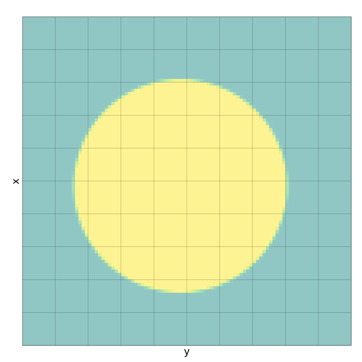


Figure 2 shows the convergence rates of the three methods in the norm. The expected decay is observed in both non-linear methods while the linear method lays behind with a decay rate of . It is relevant to note that although both non-linear methods benefit from the same rate, the associated constants differ by an order of magnitude, showing the practical improvement gained by imposing consistency. This improvement is also visible on Figure 3 which shows that in the LinearInterface method, the interfaces that minimize the error on the surrounding cells lay always inside the circle as the curvature of the boundary pushes them towards the center. On the contrary, LinearInterfaceCC seems to find the right compromise between sticking to the cell average while capturing at the same time the curvature trend hinted by the surrounding cell averages.
6 Relation to compressed sensing
6.1 Compressed sensing and best -term approximation
In this section we discuss the application of our setting to the sparse recovery of large vectors from a few linear observations. We thus take
equipped with some given norm of interest. The linear measurements of are given by
where is an measurement matrix, with typically .
The topic of compressed sensing deals with sparse recovery of from such measurements, that is, searching to recover an accurate approximation to by a vector with only a few non-zero components. We refer to [10] for some first highly celebrated breakthrough results and to [21] for a general treatment.
We define the nonlinear space of -sparse vectors as
and the best -term approximation error in the norm as
One natural question is to understand for which type of measurement matrices does the noise-free measurement contain enough information, in order to recover any up to an error . In other words, one asks if there exists a recovery map such that one has the instance optimality property at order
| (6.19) |
with a fixed constant, which we denote by . This question has been answered in [12] in terms of the null space . We say that satisfies the null space property at order with constant , denoted by if and only if
| (6.20) |
This property quantifies how much vectors from the null space can be concentrated on a few coordinates. One main result of [12] is the equivalence between at order and at order in the following sense.
Theorem 6.1.
One has and conversely .
One natural question is whether matrices with such properties can be constructed with a number of rows/measurements barely larger than . As we recall further the answer to this question is strongly tied to the norm used on .
6.2 Stability and the null space property
The nonlinear estimation results that we have obtained in §2 and §3 can be applied to the setting of sparse recovery, offering us a different vehicle than the null space property to establish instance optimality.
In the present setting, for a given norm , the stability property (1.6) takes the form
| (6.21) |
and the inverse stability property (1.7) takes the form
| (6.22) |
since for sparse vectors we have . We refer to these properties as and , respectively.
Application of Theorem 2.3 in the noiseless case immediately gives us that the nonlinear best fit recovery satisfies the instance optimality bound (6.19) with constant . In other words
| (6.23) |
The following result shows that is actually equivalent to , and thus to , in the sense that a converse result holds when is chosen to be the Riesz norm (3.10).
Theorem 6.2.
For any norm , one has
| (6.24) |
Conversely, let be the Riesz norm so that , then
| (6.25) |
Proof.
Assume that and hold. Let and its best approximation in , then
This shows that holds with .
Conversely, assume that holds. From the definition of the Riesz norm, it is immediate that holds with . For , let be the minimizer of . Then, one has
by using as a sparse approximation to . Since , this shows that holds with . ∎
6.3 The case of norms
The range of allowing the properties to be fulfilled is best understood in the case of the norms, that is , as discussed in [12] which points out a striking difference between the case and :
- 1.
In the case , it is proved that cannot hold unless . In other words, instance optimality in even at order requires a number of measurements that is proportional to the full space dimension.
- 2.
In the more favorable case , it is proved that for matrices which satisfy the -RIP property of order
with parameter , the holds with depending on . Such matrices are known to exists with rows.
Our setting based on the stability properties and applies more naturally to a different class of matrices built from graphs, which is also known to be well adapted for sparse recovery in the norm. A bipartite graph with left and right vertices, and of left degree , is an -graph expander if
where is the set of vertices connected to . We necessarily have , and . From [11], it is known that there exists a -graph expander with and .
7 Appendix: Proof of Proposition 5.1

The proof contains 15 cases, represented on a tree in Figure 4. These cases
correspond to different geometric situations, up to certain symmetries that leave the final relevant quantities
and unchanged.
Node a: Take , with ,
and denote , and , the corresponding unit vectors and offsets from the definition 5.15
of . Recalling that is the center of , we also denote
the delimiting line between and , and define in a similar way.
Case 1: If , we have
so has constant sign, which implies .
Node b: In all other cases, the cones
are non-empty, and we can define the external bisector
which is the line of symmetry between and . We also denote
Observing that
| (7.26) |
and
| (7.27) |
the stability property (5.17) can be rewritten as
or equivalently
| (7.28) |
Up to a rotation of by a multiple of , we may assume without loss of generality that
that is, is at an angle of at most with the horizontal axis, and lies above .
Take the canonical basis of .
Node c: Consider the situation where . As and , the lines and intersect at one point .
Moreover, the above condition implies . Using the fact that , we also get .
Up to a symmetry with respect to the vertical axis, we can assume that is included in the quadrant . Now consider a cell such that , then there exist points and . As and , we get , so there is at most one such cell , and inequality (7.28) reduces to
Case 2: If , then has constant sign on , so .
Case 3: If is in the central cell , the dilation of with respect to by a factor is a subset of , and the image of is in , so
Case 4: If is in the lower left cell , the dilation of with respect to by a factor is in , so
The same argument holds with instead of when is in the upper right cell. Moreover, as and go through the central cell, may not be in the upper left or lower right cells.
Case 5: If is in the lower central cell , denote the distance between and when they pass from to the central cell , and the depth of the point of intersection. Then
so . On the other hand, the parallelogram of base , of height , and with sides orthogonal to belongs to (it does not escape to the right of because is close to the horizontal axis, so the sides of the parallelogram are at an angle at most with the vertical axis), and has an area , which proves that
A similar construction can be applied to the remaining cases where is in the upper central, central left or central right cell, which concludes the proof for Node c.
Node d: If now , as , we get . Observe that since for all ,
In the same way, . We now divide into columns separated by the vertical boundaries between cells, and in addition by vertical lines where intersects the two horizontal lines separating cells of , as illustrated in Figure 7.
Let be such a column, and a cell intersecting . If , intersects either the upper or lower boundary of , but not both since is at an angle of at most with the horizontal axis. If it is the upper boundary, the symmetric of the part of above with respect to is in . If it is the lower boundary, the symmetric of the part of below with respect to is in . Using the fact that and are symmetric with respect to , we obtain
Thanks to this observation, instead of (7.28) we only have to prove the inequality
| (7.29) |
on each column separately. We thus consider only one column in the sequel, and assume up to a horizontal dilation (which preserves the condition ) that has width and is composed of three full cells.
According to the definition of the columns, there is at most one cell such that , and as separates and , it is only for this cell that we may have . If there is no such cell, (7.29) trivially holds. Otherwise, similar to Node c, we only need to prove
where is the cell containing . Denoting , , and the upper left, upper right, lower left and lower right corner points of , we observe that the assumptions on and imply and .
Node e: If , that is, if contains no intersection point between and , we match cases depending on the position of in , and of its corners with respect to . They are illustrated in Figure 8.
Case 6: If is the bottom cell and , then the two other cells are included in , so
Case 7: If is the bottom cell and but , is a triangle of width and height at most , so there is a rectangle of same width and twice as high, and thus
The same argument holds when but , and we necessarily have or in since . If is the top cell, applying a symmetry with respect to the horizontal axis and exchanging with brings us back to Cases 6 and 7.
Case 8: If is the central cell, and the two other cells are included in and , and we conclude as in Case 6.
Case 9: If is the central cell, , but , the top cell is included in , and there is a rectangle of same width and height as in the bottom cell, so
The same situation occurs when only three points among are in .
Case 10: If is the central cell, only one vertex among , is in , and only one among , is in , both and are triangles, and there exist rectangles and of same widths and heights, so
As and each contain at least one corner of , we treated all cases for Node e.
Node f: Finally, we consider the situation where there is an intersection point in , and therefore in . We again match cases, illustrated in Figure 9, depending on the position of in , and of its corners with respect to .
Case 11: If is the bottom cell, as and pass through the central cell of , is included in the central column of , and no corner of can be in , since otherwise would have to pass through that corner, according to the definition of the columns. As a consequence, and necessarily pass through the central cell of , so is a triangle, and we proceed as in Case 7. The same happens if is the top cell, so in the rest of the proof we only consider situations where is the central cell.
Case 12: If the horizontal line passing through does not intersect at any other point, is entirely above and entirely below. Denoting , the vertical dilation with respect to by a factor sends in , and the vertical dilation with respect to by a factor sends in , so
because for .
In the remaining cases, up to a symmetry with respect to the vertical axis, we can assume that and , and in particular and .
Case 13: If and , the situation is similar to Case 8.
Case 14: If and , the top cell is included in , and one of the lines or intersects the line segments and at points and . Then the triangle is included in and contains , so there is a rectangle of same width and height in . In the end
The same approach treats the symmetric case and ,
Case 15: Finally, if and , denote , , the angle between the vertical axis and the line among and that intersects , and the angle between the line among and that intersects and the horizontal axis. As , so .
We can now compute
and
If , we get
Similarly, implies . In any case, we found
which concludes the proof.
As a last remark, note that the constants and in Proposition 5.1 are sharp, since equality is attained by functions of constant sign on each cell for , and by with , and for .
References
- [1] B. Adcock, A. C. Hansen, and C. Poon. Beyond consistent reconstructions: optimality and sharp bounds for generalized sampling, and application to the uniform resampling problem. SIAM Journal on Mathematical Analysis, 45(5):3132–3167, 2013.
- [2] F. Arandiga, A. Cohen, R. Donat, and N. Dyn. Interpolation and approximation of piecewise smooth functions. SIAM Journal on Numerical Analysis, 43(1):41–57, 2005.
- [3] J.-P. Argaud, B. Bouriquet, F. de Caso, H. Gong, Y. Maday, and O. Mula. Sensor placement in nuclear reactors based on the generalized empirical interpolation method. Journal of Computational Physics, 363:354 – 370, 2018.
- [4] B. Battisti, T. Blickhan, G. Enchery, V. Ehrlacher, D. Lombardi, and O. Mula. Wasserstein model reduction approach for parametrized flow problems in porous media. working paper or preprint, May 2022.
- [5] P. Benner, A. Cohen, M. Ohlberger, and K. Willcox. Model Reduction and Approximation: Theory and Algorithms, volume 15. SIAM, 2017.
- [6] P. Berger, K. Gröchenig, and G. Matz. Sampling and reconstruction in distinct subspaces using oblique projections. arXiv preprint arXiv:1706.06444, 2017.
- [7] P. Binev, A. Cohen, W. Dahmen, R. DeVore, G. Petrova, and P. Wojtaszczyk. Data assimilation in reduced modeling. SIAM/ASA Journal on Uncertainty Quantification, 5(1):1–29, 2017.
- [8] P. Binev, A. Cohen, O. Mula, and J. Nichols. Greedy algorithms for optimal measurements selection in state estimation using reduced models. SIAM/ASA Journal on Uncertainty Quantification, 6(3):1101–1126, 2018.
- [9] B. Bojanov. Optimal recovery of functions and integrals. In First European Congress of Mathematics, pages 371–390. Springer, 1994.
- [10] Emmanuel J. Candès, Justin K. Romberg, and Terence Tao. Stable signal recovery from incomplete and inaccurate measurements. Commun. Pure Appl. Math., 59(8):1207–1223, 2006.
- [11] Michael Capalbo, Omer Reingold, Salil Vadhan, and Avi Wigderson. Randomness conductors and constant-degree lossless expanders. In Proceedings of the thiry-fourth annual ACM symposium on Theory of computing, pages 659–668, 2002.
- [12] A. Cohen, W. Dahmen, and R. DeVore. Compressed sensing and best k-term approximation. Journal of the American mathematical society, 22(1):211–231, 2009.
- [13] A. Cohen, W. Dahmen, R. DeVore, J. Fadili, O. Mula, and J. Nichols. Optimal reduced model algorithms for data-based state estimation. SIAM Journal on Numerical Analysis, 58(6):3355–3381, 2020.
- [14] A. Cohen, W. Dahmen, O. Mula, and J. Nichols. Nonlinear reduced models for state and parameter estimation. SIAM/ASA Journal on Uncertainty Quantification, 10(1):227–267, 2022.
- [15] A. Cohen and R. DeVore. Approximation of high-dimensional parametric pdes. Acta Numerica, 24:1–159, 2015.
- [16] A. Cohen, R. DeVore, and C. Schwab. Analytic regularity and polynomial approximation of parametric and stochastic elliptic PDE’s. Analysis and Applications, 09(01):11–47, 2011.
- [17] R. DeVore, G. Petrova, and P. Wojtaszczyk. Greedy algorithms for reduced bases in Banach spaces. Constructive Approximation, 37(3):455–466, 2013.
- [18] R.A. DeVore. Nonlinear approximation. Acta numerica, 7:51–150, 1998.
- [19] J. L. Eftang, A. T. Patera, and E. M. Rönquist. An ”hp” certified reduced basis method for parametrized elliptic partial differential equations. SIAM Journal on Scientific Computing, 32(6):3170–3200, 2010.
- [20] V. Ehrlacher, D. Lombardi, O. Mula, and F.-X. Vialard. Nonlinear model reduction on metric spaces. application to one-dimensional conservative pdes in wasserstein spaces. ESAIM M2AN, 54(6):2159–2197, 2020.
- [21] Simon Foucart and Holger Rauhut. An invitation to compressive sensing. In A mathematical introduction to compressive sensing, pages 1–39. Springer, 2013.
- [22] F. Galarce, D. Lombardi, and O. Mula. State estimation with model reduction and shape variability. application to biomedical problems. SIAM Journal on Scientific Computing, 44(3):B805–B833, 2022.
- [23] C. Greif and K. Urban. Decay of the kolmogorov n-width for wave problems. Applied Mathematics Letters, 96:216–222, 2019.
- [24] J. K. Hammond, R. Chakir, F. Bourquin, and Y. Maday. PBDW: A non-intrusive reduced basis data assimilation method and its application to an urban dispersion modeling framework. Applied Mathematical Modelling, 76:1–25, 2019.
- [25] J. S. Hesthaven, G. Rozza, and B. Stamm. Certified reduced basis methods for parametrized partial differential equations. SpringerBriefs in Mathematics, 2015.
- [26] T. Hrycak and K. Gröchenig. Pseudospectral fourier reconstruction with the modified inverse polynomial reconstruction method. Journal of Computational Physics, 229(3):933–946, 2010.
- [27] Y. Maday, A. T. Patera, J. D. Penn, and M. Yano. A parameterized-background data-weak approach to variational data assimilation: formulation, analysis, and application to acoustics. International Journal for Numerical Methods in Engineering, 102(5):933–965, 2015.
- [28] Y. Maday and B. Stamm. Locally adaptive greedy approximations for anisotropic parameter reduced basis spaces. SIAM J. Scientific Computing, 35(6):A2417–A2441, 2013.
- [29] Yuly Makovoz. Random approximants and neural networks. Journal of Approximation Theory, 85(1):98–109, 1996.
- [30] C. A. Micchelli and Th. J. Rivlin. A survey of optimal recovery. Springer, 1977.
- [31] O. Mula. Inverse problems: A deterministic approach using physics-based reduced models. Submitted, 2022.
- [32] E. Novak and H. Wozniakowski. Tractability of multivariate problems, volume i: Linear information, european math. Soc., Zürich, 2(3), 2008.
- [33] M. Ohlberger and S. Rave. Reduced basis methods: Success, limitations and future challenges. In Proceedings of the Conference Algoritmy, pages 1–12, 2016.
- [34] James Edward Pilliod. An analysis of piecewise linear interface reconstruction algorithms for volume-of-fluid methods. U. of Calif., Davis, 1992.
- [35] James Edward Pilliod Jr and Elbridge Gerry Puckett. Second-order accurate volume-of-fluid algorithms for tracking material interfaces. Journal of Computational Physics, 199(2):465–502, 2004.
- [36] Elbridge Gerry Puckett. A volume-of-fluid interface tracking algorithm with applications to computing shock wave refraction. In proceedings of the fourth international symposium on Computational Fluid Dynamics, pages 933–938, 1991.
- [37] G. Rozza, D. B. P. Huynh, and A. T. Patera. Reduced basis approximation and a posteriori error estimation for affinely parametrized elliptic coercive partial differential equations. Archives of Computational Methods in Engineering, 15(3):1, 9 2007.
- [38] Jonathan W Siegel and Jinchao Xu. Sharp bounds on the approximation rates, metric entropy, and -widths of shallow neural networks. arXiv preprint arXiv:2101.12365, 2021.
- [39] H. Tran, C. G. Webster, and G. Zhang. Analysis of quasi-optimal polynomial approximations for parameterized pdes with deterministic and stochastic coefficients. Numerische Mathematik, 137(2):451–493, 2017.
- [40] G. Welper. Transformed snapshot interpolation. arXiv preprint arXiv:1505.01227, 2015.
- [41] Z. Zou, D. Kouri, and W. Aquino. An adaptive local reduced basis method for solving pdes with uncertain inputs and evaluating risk. Computer Methods in Applied Mechanics and Engineering, 345:302–322, 2019.