Finite- and Large-Sample Inference for Model and Coefficients in High-dimensional Linear Regression with Repro Samples
Abstract
In this paper, we present a novel and effective inference approach to conduct both finite- and large-sample inference for high-dimensional linear regression models. This approach is developed under the so-called repro samples framework, in which we conduct statistical inference by creating and studying the behavior of artificial samples that are obtained by mimicking the sampling mechanism of the data. We constr confidence sets for (a) the true model corresponding to the nonzero coefficients, (b) a single or any collection of regression coefficients, and (c) both the model and regression coefficients jointly. To facilitate the constructions of these confidence sets and overcome computational difficulties of searching all possible models, we use an innovative Fisher inversion technique to construct a model candidate set that includes the true sparse model with the probability close to 1 for models with both Gaussian and non-Gaussian errors. The proposed approach fills in two major gaps in the high-dimensional regression literature: (1) lack of effective approaches to addressing model selection uncertainty and providing valid inference for the underlying true model; (2) lack of effective inference approaches to guaranteeing finite-sample performance. We provide both finite-sample and asymptotic results to theoretically guarantee the performance of the proposed methods. In addition, our numerical results demonstrate that the proposed methods are valid and achieve better coverage with smaller confidence sets than the current state-of-the-art approaches, such as debiasing and bootstrap approaches.
and and
??Department of Operations, Business Analytics and Information Systems,University of Cincinnati, Cincinnati, OH 45221, USA. ??
??Department of Statistics, Rutgers University, New Brunswick, NJ 08854, USA. ??; ??
1 Introduction
High-dimensional linear regression plays an important role in modern statistics, with applications ranging from signal processing [59] to econometrics [3, 33] to bioinformatics [56]. There has been a large amount of literature on this topic in the past 30 years. The earlier research focused more on estimation/detection problems such as coefficients estimation [9, 53] and support recovery [66, 71]. Starting with the work of debiased Lasso [63, 44, 32], the more difficult task of inference comes to the central stage. Some recent works on inference include confidence interval construction [63, 44, 32], multiple testing of regression coefficients [40], and post-selection inference [51, 54, 36].
Despite many works on the topic, several important open problems remain. First, most existing works focus on the inference for regression coefficients, while the inference for true model (including uncertainty quantification for model selection) in the high-dimensional regression model is mostly absent. This is partly due to the challenges arising from the discrete nature of the model space, which makes the conventional inference tools built for continuous parameters, such as the central limit theorem and bootstrap theorems, inapplicable. Furthermore, all the results in the literature on high-dimensional inference are asymptotic, assuming the sample size goes to infinity, and there are no theories concerning the performance of these procedures under finite-sample settings. The performance of these asymptotic procedures is frequently empirically unsatisfactory, especially when sample size is limited. Thus a procedure with guaranteed finite-sample performance is desirable. Finally, the post-selection inference framework attempts to sidestep the problem of model uncertainty by only making conditional inferences for regression coefficients of the predictors selected by a model selection procedure. If some predictor variables are significant but not selected, no inference results are available on these predictors and we may miss some important signals.
To solve the above problems, we develop a repro samples method that quantifies both the uncertainty in model selection and that in estimation of regression coefficients and their functions. Specifically, we provide a comprehensive inferential approach with which we can construct confidence sets for (a) the true model, (b) a single or any collection of regression coefficients, and (c) both the model and regression coefficients jointly. Moreover, the proposed repro samples approach enjoys finite-sample performance guarantees without requiring a large sample size for all of (a)-(c). Although our work focuses primarily on finite-sample performances, we also provide related large-sample results.
Consider the high-dimensional linear regression problem where we observe an response vector with an design matrix , where Suppose that the observed relates only to a subset of predictor variables indexed by with
| (1) |
Here, is the realization of the error term, are unknown model parameters, , and . Corresponding to model (1), there is a random sample (or population) version of data generation model
| (2) |
of which model (1) is a realization. In general, we assume , although further conditions may be required for different inference tasks.
To carry out the inference tasks, two inversion techniques are devised in the proposed repro samples method to handle the discrete parameter . The first inversion technique, developed in Section 2 and referred to as Fisher inversion, aims to obtain a model candidate set that includes the true with a high (close to 1) probability using the observed data and a large set of reproduced (simulated) artificial error terms. This model candidate set, typically of a reasonable size, is then used to facilitate the constructions of level- confidence sets and intervals later in Sections 3 and 4. To obtain a level- model confidence set for in Section 3, we use the second inversion technique, referred to as Fisher-Dempster inversion for distinction, to overcome the difficulty that the central limit theory does not apply on a discrete parameter space. The Fisher-Dempster inversion technique inverts a level- Borel set of possible error realizations to get a level- confidence set for . Unlike the conventional Wald-test type of methods, the proposed repro samples method directly provides the desired confidence sets without having to estimate or any other model parameters.
1.1 Contributions
To summarize, this paper has the following contributions.
- 1.
We propose a repro samples method to effectively construct model confidence set and quantify model selection uncertainty for the high-dimensional linear regression model. To the best of our knowledge, it is the only computationally efficient approach that provides a performance-guaranteed model confidence set for without data splitting or a prior assumed candidate model set.
- 2.
We develop a novel inference procedure for regression coefficients . Contrary to other existing methods, our approach does not rely on covariance matrix estimation or a consistent model selection procedure. Therefore, it sidesteps potential issues caused by any inaccurate estimation of the covariance matrix or mis-selection of the model.
- 3.
We propose a novel and efficient way to find candidate models using synthetically generated residuals. Theoretically, we show that this set of candidate models have a high probability to include the true model for both Gaussian and non-Gaussian errors, and we also provide an upper bound for the expected size of the set. Numerically, we have shown in our simulation studies that the proposed model candidate set is of reasonable size, and covers with a probability close to 1 even in challenging settings. The model candidate set facilitates the inference for both the true model and the regression coefficients. It can also be used for variable screening, providing superior performances to the traditional screening approaches relying on only marginal relationship.
- 4.
Theoretically, we show that the proposed inference procedures for both the model and the regression coefficients achieve finite-sample coverage guarantees, while most literature on high-dimensional models focuses only on asymptotic properties. To our knowledge, the proposed method is the first approach that guarantees coverage for finite samples. Additionally, our theory suggests a complementary effect between computational power and sample size: one can achieve valid coverage as long as either is sufficiently large.
- 5.
Theoretically, we do not need to impose the standard conditions that high-dimensional statistics literature typically requires to obtain a consistent estimation, such as the restricted isometry property or restricted eigenvalue conditions [5, 63]. Neither do we need to require signal strength conditions [66, 5], which is usually necessary for consistent model selection. We also provide a discussion on conditions required for different implementations of the proposed procedure under computational considerations.
- 6.
Finally, through extensive numerical studies, we show that the proposed method produces better performed confidence sets than those of the state-of-the-art debiased Lasso estimators [63, 32]. Because of the finite-sample validity guarantee, our method achieves the desired coverage even in small-sample regimes, while the existing methods can not.
Overall, we provide a comprehensive framework that subsumes existing inference approaches by two means: we consider a broader set of marginal and joint inference problems to account for uncertainties of estimating both the model and the regression coefficients; and we provide supporting theories to guarantee both finite- and large-sample performances.
1.2 Related works
There has been much effort in recent years to develop inference procedures for regression coefficients or functions of in high-dimensional linear regression models. On the inference for a single coefficient parameter, [63, 55, 32] propose the debiased Lasso estimator and develop its asymptotic distribution. Other works along this line include [10, 16, 17, 12, 13]. Moreover, [70, 65, 18, 7, 44, 67, 69] investigate simultaneous inference on a subset or all of Additionally, quadratic and more general functions of have been studied in [1, 24, 30, 68, 69, 43]. However, all the existing approaches are developed using large-sample theories and do not have any finite-sample performance guarantees. The inference for , on the other hand, is almost entirely absent in high-dimensional statistics literature, although there are a few works in low-dimensional setting. [26, 22] construct a model confidence set utilizing sequential testing procedures against a pre-specified finite-dimensional full model, which cannot be well-defined in the high-dimensional setting. [38] proposes a novel concept of model confidence bounds to confine within a pair of nested models. However, the method relies on selection consistency and bootstrap validity, and is computationally expensive for high-dimensional data.
A recent work by the authors [62] provides a repro samples framework for statistical inference under a general setup, in which the number of parameters is less than the number of observations . The current paper focuses on the high-dimensional case that was not discussed in [62]. New procedures and theoretical results with conditions tailored to high-dimensional models that guarantee the performance of the proposed method in both finite and large-sample cases are developed. Finally, as discussed in [62], the repro samples approach is related to other modern simulation-based procedures, such as the bootstrap [19, 10], the approximate Bayesian computation [2, 14], the inferential models [42] and the generalized fiducial inference [25], where artificial data are used to address inference problems.
1.3 Notation
For any , we let . For a vector , we let be the -th entry. For a set , let be the cardinality of . For two positive sequences and , write , if ; write , if . We use for probability and for expectation and add subscripts (eg., and ) to indicate source of randomness. We use and for empirical probability and expectation. For a and , we use to denote the sub-vector of , containing the entries of that are associated with the indices in . The model space For a matrix , let be the vector space spanned by the columns of : . We also call the projection matrix of , and is the identity matrix. Lastly, we use and to denote the level- confidence set for , and , respectively, where is any subset of . Here, the superscript of simply indicates the target parameter of the confidence set is , and the set does not depend on any particular value of . Notations for other confidence sets, such as , , etc., are defined similarly.
Finally, we refer to a simulated copy of artificial as a repro copy of the realized and the artificial data as a repro sample of for a potential set of values . The key of our approach is to study and relate this with and the with . We generally refer to our method, developed by using the copies of and as a repro samples method. We will provide more details in each of the sections.
1.4 Organization
The paper is organized as follows. Section 2 provides a data-driven approach to effectively construct a set of candidate models that will include the true model with a high (close to 1) probability. Section 3 utilizes the candidate set to construct a level- confidence set for , and provides both finite-sample and large-sample guarantees. Section 4 studies the inference problems of regression coefficients, including inference for linear transformations of and functions of . Section 5 provides numerical illustrations of the proposed methods and compares the coverage and size of the constructed confidence sets with the bootstrap and state-of-the-art debiased Lasso methods. In Section 6, we perform a real data analysis. Section 7 concludes the paper with a discussion of our results and future research directions. Theoretical proofs, technical lemmas, as well as additional discussions and numerical results are deferred to Appendices A–F in the supplementary materials.
2 Finding candidate models for
In this section, we propose a novel procedure to efficiently find possible candidate models for In Section 2.1, to rigorously set up our problem and eliminate possible non-identifiability issues, we formally define the target true sparse model as the smallest model that generates the data. Section 2.2 introduces an effective computing algorithm and Fisher inversion method to obtain a set of candidate models for . Section 2.3 proves that the model candidate set obtained in Section 2.2 is guaranteed to cover with a probability close to 1 under the Gaussian error model assumption, in both finite-sample and asymptotic settings. Moreover, we also provide a theoretical upper bound for the size of the model candidate set. In Section 2.4, we show that the finite-sample coverage results also hold when the error term follows a number of other distributions, such as when is heterogeneous, Cauchy, -distributed, contaminated Gaussian or sub-Gaussian distributed. In addition, we show that the large-sample result continues to hold under sub-Gaussian errors.
2.1 Identifiability and definition of
Under the high-dimensional setting with , there might be another model and corresponding coefficients such that . Even when we know both and the realized noise , it is not possible to tell apart and , since We refer to this as an identifiability issue. To address this issue and uniquely define , the conventional practice in the high-dimensional regression literature [53, 5, e.g.,] is to favor the smaller model, since as stated in [53], in real applications researchers would often prefer and be interested in the simplest (smallest) model that generates the observed data for better prediction performance and model interpretation. Commonly used penalized regression approaches, such as Lasso [53], SCAD [20], and MCP [64], all employ penalty terms designed to favor smaller models. In this paper, to address this identifiability issue, we follow the same practice to rigorously re-define as the smallest model among the set :
| (3) |
Throughout the paper, we assume that the true model defined in (3) is unique, which we refer to as the identifiability condition. For notational simplicity, we will still refer as and as in the remainder of the paper. Our inference target is this set of just defined.
Furthermore, we follow [49] to define the degree of separation between model and other models of equal or smaller model sizes as
Under the identifiability condition mentioned above, we have . The notion is related to of the -min condition in the literature [53, e.g.,]. However, unlike the existing literature, we do not impose any assumption on other than that .
2.2 Algorithm for finding candidate models
Here, we use an inversion method to construct a set of candidate models for . To illustrate the basis of this inversion method, we first show that we can recover the true model in an ideal (unrealistic) case assuming that the realization of the error term is known. In particular, Lemma 1 below states that defined in (3) can be expressed in terms of the given realization using an optimization statement.
Lemma 1.
Let be the projection matrix of and be the projection matrix of Let Then, given , defined in (3) satisfies
| (4) |
and moreover for any
In practice, however, we do not know the realized errors so we cannot directly apply Lemma 1. Nonetheless, equation (4) offers guidance on constructing a set of candidate models for More specifically, we generate a large number of, say , copies of Monte Carlo . Then instead of solving (4) with the realized we compute
| (5) |
for each After that, we collect all ’s to form a candidate set for :
| (6) |
Since the mapping function from to in (5) is a many-to-one mapping, many of the copies of ’s obtained by (5) are identical. The size is often much smaller than . See Theorem 3 of Section 2.3 for a theoretical result on the size of the candidate set.
The only difference between (5) and (4) is that we replace with Since the mapping function from to in (5) is many-to-one, many ’s that are close to each other map to an identical . One could imagine that if some is in a neighborhood of , then for such ’s, the event is very likely to happen. The size of such a neighborhood depends on the separation metric and the sample size, yet its probability measure is always positive under the identifiability condition described in Section 2.1. As a result, as long as , the number of repro copies, is sufficiently large, eventually some will fall in this neighborhood, leading to and hence the candidate set contains the true model . Formal theorems that support this method for different error distributions are presented in Section 2.3–2.4.
To put it succinctly, we summarize the aforementioned procedure in Algorithm 1 below.
Remark 1.
[Practical implementation of Algorithm 1] When we implement Algorithm 1, we need to consider two practical issues: a) how to handle the tuning parameter in the penalty term, and b) solving an optimization problem with a penalty is often computationally difficult for high-dimensional data. In our implementation in the numerical study Sections 5 and 6, we follow common practices in the literature to handle these two issues. First, it is common to use a selection criterion to determine the value of the tuning parameter [11, 20, 53]. We use the extended BIC (EBIC) [11] to determine , due to its good empirical performance and asymptotic model selection consistency in high-dimensional settings. Second, solving an optimization problem with the penalty is computationally expensive and yields unstable results [41]. In practice, researchers often use a surrogate to replace the penalty. In our numerical studies, we adopt the adaptive Lasso [71] as a surrogate for the penalty in (5) because of its simplicity and convexity. One may also use other surrogates like the truncated Lasso penalty [50], smoothly clipped absolute deviation penalty (SCAD) [20], or the minimax concave penalty (MCP) [64], among others. Although computationally more efficient, using some of these penalties may require us to make additional assumptions on the design matrix. See Remark 2 for further discussions. In this paper, we develop our general theories using the penalty and constraint rather than a specific surrogate penalty function, since we would like to understand the fundamental properties and allow for the flexibility of using any penalty or constraint within the proposed repro samples framework.
Equations (4) and (5) are inversion operations that solve for when given and the error term . The difference is that (4) assumes the realized is known while (5) uses a simulated . This technique of using a random to replace in an inversion can be traced back to Fisher’s fiducial inference [25, 52]. Therefore, we refer to the inversion method used in Algorithm 1 as Fisher inversion. Here, we use it to assemble potential candidate models for , which reduces the size of the effective model space from to . In Section 3, we will develop a different inversion technique to construct the level- confidence set for .
2.3 Theoretical results for models with Gaussian errors
In this subsection, we present theoretical guarantees of our method under Gaussian error , and extend the results beyond the Gaussian error model in the next subsection. Here, we show in Theorems 1-2 that in the following two cases: 1) the sample size is finite and , 2) is finite and , respectively. The probability refers to the joint distribution of and where is a Monte Carlo copy of
Theorem 1.
Theorem 2.
The two theorems above suggest two complementary driving forces of the coverage validity: the sample size and the computation time measured by . In cases when the sample is limited, Theorem 1 implies that we can recover the signal with a valid coverage as long as the computation time (linearly scaled with ) goes to infinity; in cases when the computational resources are limited, Theorem 2 then indicates collecting sufficient samples will result in a valid coverage guarantee. In Theorem 1, for any finite , the lower bound for is of the same order as and the upper bound is of the same order as Therefore the range of always exists for a that is small enough. In Theorem 2, the existence of the range of follows from when is large enough. Therefore, in both theorems, the required range for is a non-empty interval of positive length, although this interval is smaller for a smaller
Remark 2.
In this paper, we develop our general theorems using the penalty or constraints, rather than any specific version of surrogates, to keep the theory general and allow researchers to select the surrogate that best suits their needs. In our implementation in the paper, we used the adaptive Lasso penalty as a surrogate for the penalty since it is computationally efficient and performs comparably to commonly used non-convex penalties. To obtain similar result of Theorem 1 tailored specifically for the adaptive Lasso penalty, we would need impose an additional condition called the minimum adaptive restrictive eigenvalue condition [5, Ch 6& 7]. This condition is similar, but slightly weaker than the restricted strong convexity and it is also weaker than the irrepresentable condition [5, Ch 6& 7]. Moreover, the simulation results of Model (M5) in Section 5 suggest that our current implementation of the repro samples approach still performs well empirically even when the minimum adaptive restricted eigenvalue condition required for the adaptive Lasso does not hold. Besides the adaptive Lasso, there are other possible surrogates (e.g., Lasso, adaptive Lasso, SCAD, MCP, etc.) for the penalty. Whether we need additional conditions on the design matrix and what these conditions are depend on the specific surrogate we use in our implementation. In general, there is a trade-off between additional conditions required and computational cost. For example, if we choose to adopt the truncated Lasso penalty (TLP) proposed by [49], then no additional condition is required on the design matrix. Alternatively, we can choose to use a constrained least squares approach as opposed to the penalized approach (see Appendix A for the formulation and theories regarding the constraint approach). In this case, if we choose to use the constrained regression to estimate the models, which we can achieve with the modern mixed integer optimization approach [4], we would not need any condition on the design matrix either. However, both of these approaches demand substantially higher computational cost compared to a convex penalty function like the adaptive Lasso.
Besides the coverage results above, another important aspect is the size of the candidate set Theorem 3 below provides a theoretical bound for the expectation of the size of the model candidate set . In the theorem, for any model with we define the model distance between and the truth as
Theorem 3.
Let be the set of smaller than that are close to Then for where
where where is the number of repro samples used in Algorithm 1.
Intuitively, if an alternative model is closer to in that is small, it should be more likely to be included in the model candidate set Therefore the candidate set would include models that are close to , and models that are farther away from would be included with a smaller probability. As a result, the size of the candidate set depends on (a) how many models are close to , (b) the probability of other models included. This intuition is verified explicitly by the result in Theorem 3. Specifically, if , then with high probability, the candidate set will include all the models with where is the number of repro copies in Algorithm 1, and it will include those with with a positive probability. The larger the is, the smaller the probability being included. Moreover, a larger sample size leads to smaller model selection uncertainty, typically resulting in a smaller candidate set, aligning with our expectations. Additionally, the impact of the repro sample size on the size of is logarithmic. Finally, we see from Theorem 3 that the contribution to the cardinality of the model candidate set from all models larger than is bounded by , therefore the candidate models include only models of size similar or smaller than with probability close to 1 due to the regularization in Step 2 of Algorithm 1.
2.4 Heterogeneous, non-Gaussian and sub-Gaussian error models
In this subsection, we show that even when the model error assumption is violated, the model candidate set obtained using Algorithm 1 with can still cover the true model with a high probability.
We first show in Theorem 4 below that the results in Theorem 1 still hold when the linear model in (2) is now generalized to the following,
| (9) |
Here, the error term , and is an fixed vector with each or a random vector independent of , with each
Theorem 4.
The above theorem shows that when the error term is generalized from to the candidate set still cover the truth with an arbitrarily high probability, as long as is large enough. The generalized error term covers a wide range of non-Gaussian error models, including heterogeneous variances, Cauchy distribution, -distribution, contaminated Gaussian distribution, etc. Below, we discuss how these non-Gaussian errors are connected with
-
Heterogeneous Variance. In this case, where Therefore we can just make fixed such that .
-
Cauchy Distribution. When the error is Cauchy distribution, we can simply make where are i.i.d.
-
T-distribution with degree of freedoms . Since random variables with -distribution can be formulated by a ratio of a normal random variable and the square root of a Chi-square random variable divided by its degree of freedom, we make
-
Contaminated Gaussian Distribution. In cases where some observations are contaminated, leading to a larger variance for the contaminated samples, we can make where is a constant, usually larger than 1, and are i.i.d Here represents the proportions of contaminated distributions.
-
Combination of the above. This is when follows a mixture of the above distributions.
Sub-Gaussian error models are another set of non-Gaussian error models used in high-dimensional settings due to their flexibility and robustness. We show that the results of Theorem 1 and Theorem 2 still hold for the sub-Gaussian error models, and thus candidate set obtained in Algorithm 1 can still cover the true with a high probability.
Theorem 5.
Suppose is generated by (2) with being a sub-Gaussian vector with sub-Gaussian norms bounded by a universal constant, and For any , there exists a constant and such that when the finite-sample probability bound that the true model is not included in the model candidates set , obtained by (6) with the objective function (5), is as follows,
| (10) |
Therefore as where is arbitrarily small.
For the model candidate set in both theorems, the repro errors used in Algorithm 1 are still sampled from , even though the true underlying is not. This is possible because is a vector in , as long as is not too extreme, we often can find some in its neighborhood when . Under the non-Gaussian settings considered in Theorems 4 and 5, we are able to quantify such a neighborhood of that also maps to . A nice implication of these results is that we do not need to know exactly the error distribution of the model, as long as it is one of those in Theorems 4 and 5, the model candidate set obtained by Algorithm 1 contains the true with a high probability. Furthermore, we later extend the finite-sample result here to arbitrary error distributions with finite second moments; see the Discussion section.
Theorem 6.
Suppose is generated by (2) with being a sub-Gaussian vector with sub-Gaussian norms bounded by a universal constant and for a positive constant . Then the probability bound that the true model is not included in the confidence set , obtained by (6) with the objective function (5) for any finite is as follows,
Therefore for any as , if and when is large enough.
The above theorem extends the result in Theorem 2 to models with sub-Gaussian errors. It indicates that when sample size is large, we can recover the truth with Algorithm 1 with a limited number of repro samples for models with sub-Gaussian errors. Similar to the implications of Theorem 4 and 5, here we do not need to know the distribution of , and only require to be sub-Gaussian.
3 Construction of a level- Model Confidence Set
In this section, we construct a level- confidence set for model by developing a conditional repro samples method tailored to the problem. Here, we assume .
For the ease of presenting the general idea of the repro samples method as described in [62], let us first assume that we are interested in making a joint inference about and describe how the method proceeds in this case. The idea is that given any possible value of the parameters , we create an artificial repro sample data where If is close to and is equal or close to , then we expect and to be equal or close. Inversely, for a given value , if we can find a likely matching such that matches (i.e., ), then we cannot rule out that this is a potential value of . Mathematically, we define
| (11) |
Here, the function is referred to as a nuclear mapping function and the set is a fixed level- Borel set in such that
| (12) |
Again, we clarify that the in the superscript of simply indicates the target parameter is and in (11) does not rely on any particular value of
The repro samples method uses , for each given value , as a way to quantify the uncertainty of thus also the uncertainty of . Moreover, for any nuclear mapping function , as long as we have a set such that (12) holds, we can show that the set in (11) is a level- confidence set [62]. Here, the role of under the repro samples framework is similar to that of a test statistic under the classical (Neyman-Pearson) hypothesis testing framework. Besides, a good choice for is problem-specific. Effectively, the operation in (11) can be considered as an inversion operation that maps a set of to a set of . Such a mapping is a key element of the Dempster-Shafer calculus [48, 42]. To distinguish the Fisher inversion method introduced in Section 2 that produces a model candidate set, we refer to the techniques used in this section to produce a level- confidence set for as Fisher-Dempster inversion.
Our goal in this section to make inference only for the true model with being the unknown nuisance parameters. First, we write , for a . This is a copy of artificial data generated from a given set of parameters . The corresponding random version is
| (13) |
Then based on the artificial repro sample data one can obtain an estimate of , denoted by In this paper, we use
| (14) |
although in principle we can choose to use another estimator of reasonable performance. We thereafter use (14) to define the nuclear mapping function as Then we need to find a Borel set that satisfies (12), i.e., for the nuclear mapping defined above. However, the distribution of involves all of the parameters , including the nuisance parameters and . Therefore, directly obtaining for all values of is computationally challenging, if not infeasible.
Since it is not feasible to search through the entire space of , we introduce below an effective conditional repro samples method to handle the nuisance parameters and construct a level- confidence set for . The idea is to first find a quantity , such that the conditional distribution of the nuclear statistic given is free of the nuisance parameters . For now, assume we have such ; we will discuss how to obtain for our purpose later in the section. Then, based on the conditional distribution of , we construct a Borel set that depends on , the value of the random quantity , but not on , such that
| (15) |
Accordingly, the marginal probability
Now, instead of directly following (11), we construct a subset in the model space :
| (16) |
The following theorem suggests that constructed above is a level- confidence set for the true model .
Theorem 7.
The remaining task is to find the random quantity and a Borel set such that the conditional distribution of is free of the nuisance parameters and the inequality (3) holds. Note that we can rewrite (13) as , where is the projection matrix of . Write and . We have
| (17) |
In this equation, the “randomness” of (and also ) are decomposed into three components, and . Under (13), is a sufficient statistic and the last piece is an ancillary statistic that is free of the nuisance parameters . Based on this partition, we define . It then follows immediately that the conditional distribution of is free of so is the conditional probability mass function of given ,
| (18) |
for any . Note that, when given , we can use the model equation (13) to generate many copies of by repeated draws from . Therefore we can obtain the conditional probability mass function in (18) through a Monte-Carlo method.
We therefore define the Borel set as
| (19) |
In the proof of Theorem 7 in Appendix C, we prove that the conditional probability
| (20) |
It follows that, marginally, Then by (3) and using the candidate set , we propose the following confidence set for
| (21) |
To obtain the above confidence set, we use a Monte-Carlo method to compute the conditional probability in (18). We summarize the procedure of constructing the above model confidence set in Algorithm 2, with the size of the Monte-Carlo simulations
| (22) |
Theorem 8 below states that in (21) is a level- confidence set for with a guaranteed finite-sample coverage rate, as long as , the number of repro samples used to construct the candidate set in Algorithm 1, is large. Theorem 9 states that even when is limited, is still a level- confidence set for if we have a large sample size
Theorem 8.
Under the conditions in Theorem 1, for any finite and , and arbitrarily small , the coverage probability of model confidence set constructed above is as for some . Further
Theorem 9.
Under the conditions in Theorem 2, for any finite , the coverage probability of model confidence set constructed above is as for some . Further
Remark 3.
When the error is non-Gaussian, the theoretical results in Section 2.4 show that the model candidate set itself, constructed in Algorithm 1, is a valid but conservative confidence set for , even without knowing the distribution of It is challenging to derive a tighter model confidence set with a closer-to-level- coverage in cases when the distribution of is unknown, since we often need the knowledge of ’s distribution to obtain in (3) to quantify the uncertainty of . This is because both and are discrete, and typical concentration inequalities or central limit theorem do not apply. When the distribution of is known but non-Gaussian, the approach in Algorithm 2 is not valid anymore because the independence among the three components in the decomposition (17) does not hold. In such cases, a profiling approach as described in [62, 28] can be potentially applied instead, although it may pose computational challenges and yield less efficient results. Alternatively, since we now have a model candidate set with a high coverage probability, we may follow [35] to construct a distribution-free confidence set for the best working models, that is, the model that provides the best predictive performance. The idea is to construct a confidence interval for the smallest cross-validation error, and use that to construct the confidence set for the best predictive model. Since the candidate models are low-dimensional and covers the truth with a high probability, we believe that is very likely to be the best predictive model among all the candidates. The theoretical justification and the coverage of this confidence set constructed using the “best predictive model” is an intriguing future research topic.
4 Inference for regression coefficients accounting for model selection uncertainty
Section 4.1 proposes a confidence set for any subset of that accounts for model selection uncertainty, and extend the work to make inference for any linear transformation of . Section 4.2 discusses two special cases of practical importance: (a) inference for a single regression coefficient and (b) joint inference for all regression coefficients . Note that, most existing methods focus only on one of the two special cases, and there are few effective approaches on making inference for any subset or linear transformation of in the literature. Moreover, our work guarantees both finite-sample and large-sample coverage, while existing methods provide only asymptotic inferences. In Section 4.1– 4.2, we assume that the error terms are Gaussian . In Section 4.3, we extend the confidence sets for the regression coefficients in Section 4.1 to cases where non-Gaussian errors are present. Due to space limits, we defer the joint inference for the model and regression coefficients to Appendix B.
4.1 Inference for a subset of regression coefficients
Let be a collection of ’s that are of interests, where the index set . The remaining parameters , and are nuisance parameters. The subset is given based on the problem of interest, and it may overlap with or separate from . Here our strategy is to first remove the influence of the nuisance parameters and by defining a nuclear mapping function that only involves , where is a potential value of . The role of the nuclear mapping is similar to test statistics in the classical hypothesis testing framework, but in general, the definition of the nuclear mapping is broader and more flexible than the definition of test statistics. See [62] for a detailed discussion. We then utilize the model candidate set constructed in Section 2 to handle the impact of , leading to a valid confidence set for .
For a given , we define the nuclear mapping as follows
| (23) |
where is the projection matrix of and is the projection matrix of We can rewrite the above nuclear mapping as a function of :
| (24) |
Since when and for any the distribution of the nuclear mapping defined above is we let the Borel set be such that We can show that a valid level- repro samples confidence set for is
| (25) |
Now with both and out of the picture, we need to deal with the only remaining nuisance parameter To handle the impact of we utilize the model candidate set constructed in Section 2.2 and take a union approach. That is, for certain , if is defined above for any in the candidate set we then retain the in the confidence set for Specifically,
| (26) |
Note that this confidence set is a union of multiple smaller sets. This is different than confidence sets produced by existing methods which are often single intervals or ellipsoid sets. An illustration of such a confidence set is provided in the special cases that , please see Figure 1 of Appendix F.
We observe that inside the union in (4.1), each set is a confidence set based on certain low-dimensional model in the candidate set Although we do not know the true underlying model , with Algorithm 1, we are able to construct a candidate set of reasonable size that would include with a high probability. This enables us to guarantee the coverage rate, both in finite samples and asymptotically, as indicated in the following theorems.
Theorem 10.
Theorem 11.
Remark 4 (Extension to make inference for any linear transformation of ).
Let be a linear transformation of where is a transformation matrix. Let
and The inference for based on the data is now equivalently transformed to the inference for a subset of based on the transformed data Therefore we are able to construct the confidence set for by applying (4.1) on Note that one should also derive the candidate set from the transformed data using Algorithm 1.
4.2 Two special cases of interest
As stated in [63, 32], we are often interested in marginal inference for a single regression coefficient in practice. Another interesting inference problem that has been studied in the literature is to jointly infer all regression coefficients [65, 18]. In this subsection, we consider these interesting special cases and provide a new solution using the repro samples method.
Inference for a single regression coefficient. To obtain the repro samples confidence set for we simplify the nuclear mapping function defined in (23) and (24) by making . For a given , it is
|
, |
where is the projection matrix of , and Note that for the nuclear statistics is equivalent to the square of -statistics for testing , obtained by fitting a linear regression of on
Then following (4.1), we obtain the confidence set for
| (27) |
where we let Then by Theorems 10 and 11, is a level- confidence set for .
Remark 5 (Comparison with the debiased method).
We discuss the difference between our method and the debiased Lasso. First of all, our method offers the finite-sample coverage guarantee, while the debiased Lasso method can only achieve the asymptotic coverage rate. More specifically, the debiased Lasso method needs the sample size to make sure the bias, which comes from the regularized estimation and is of order , goes to 0. In contrast, our method bypasses the estimation step and constructs the confidence sets directly via the repro sampling framework, and is therefore unbiased in nature. Second, the debiased Lasso method [32] is designed to make inferences for an individual regression coefficient. The idea of the debiased Lasso method was later generalized to make inferences for functions of the regression coefficients, such as co-heritability[24] and group inference statistics [23]. However, such a generalization relies on specific forms of the functions and does not allow arbitrary functions. Our method, however, as we will show in Remark 6, can be used to construct the confidence sets for arbitrary functions. Third, we will show in Section 5.2 that, when the sample size is small, the debiased Lasso method may have either coverage issues or overly large intervals for large regression coefficients. In contrast, our method achieves the nominal coverage for both large and zero regression coefficients in the small sample setting with preferable interval lengths. See Section 5.2 for more details.
Joint inference for all regression coefficients. Let and we make joint inference for all regression coefficients here. Note that , so Following (23) and (24), the nuclear mapping function for is
| (28) |
We then let the Borel set be and construct the joint confidence set for following from (4.1),
| (29) |
Again, following Theorems 10 and 11, is a level- confidence set for the entire coefficients vector . In addition, to better understand the confidence set in (4.2), we have presented a visualization of (4.2) for an example in Appendix F.
Remark 6 (Extension to inference for any function of ).
4.3 Extension to models with non-Gaussian errors
In this section, we extend the confidence set for the regression coefficients in (4.1) to models with non-Gaussian errors. We first introduce the following corollary.
Corollary 1.
Let be a data-dependent set of that also depends on a given model and let be the coverage probability for given the true model then the confidence set for constructed by has a coverage rate bounded by
The above corollary implies that models with non-Gaussian errors can still follow the idea in (4.1) to construct confidence sets for the regression coefficients. This is because the model candidate set proposed in Section 2.2 still covers the true model with a high probability according to the results in Section 2.4 for common non-Gaussian errors. Once we have a candidate set that guarantees to cover the true model such that is close to 0, all we need is a valid inference approach in low-dimensional settings that can achieve the desired coverage given In other words, we only need a data-dependent set given a low-dimensional model namely such that given the true model, is a valid confidence set for with a desired coverage rate of (approximately) It then follows immediately from Corollary 1 that is a valid level- confidence set for
Fortunately, such a is not difficult to find, since the inference for linear models with non-Gaussian errors in low-dimensional settings have been extensively studied. For example, [34] proposed a likelihood-based approach for and errors, and [45] provided a thorough review on different approaches to deal with non-Gaussianity in the error terms of linear models. To make inference for a model with contaminated errors, see [37, 15] and the reference therein. For sub-Gaussian errors, it is well known that most of the results for Gaussian errors hold asymptotically due to the central limit theorem [60].
5 Simulation studies
In this section, we conduct simulation studies to evaluate the numerical performance of the proposed repro samples methods. The synthetic data are generated from the following five models:
- (M1)
(Extremely high dimension) Let . For , the correlation between and is set to . We set and .
- (M2)
(Decaying signal) Let For , the correlation between and is set to . We let and .
- (M3)
(High-dimensional, decaying signal) Let The correlation between and is . Let and .
- (M4)
(From [38] with many signals, but changed to create a high-dimensional setting with ) Let the true values , where the first coefficients , for , and remaining , for . For , the correlation between and is set to . We let and .
- (M5)
(Perfect colinearity, restricted eigenvalue conditions do not hold) Let the true values . For , the correlation between and is set to . To create perfect collinearity, we set such that the restricted eigenvalue condition does not hold, and We set and .
The first model (M1) represents an extremely high-dimensional setting with The second model (M2) represents a challenging case of decaying signals with the weakest one just 0.6. We set (M3) by increasing the dimension of (M2) to study the performance of the proposed approach when both a high-dimensional design matrix and weak signals are present in the data. We also add a strong signal of so the range of signal strength is from to . Model (M4), a high-dimensional adaptation of the scenario (f) in [38], features a setting that involves many true signals. Finally, we present an extremely challenging case in (M5), where typical conditions in the literature such as the restricted eigenvalue condition do not hold anymore. We replicate the simulation for 200 times for each model.
5.1 Model candidates and inference for the true model
We first study the numerical performance of the data-driven model candidate set in (6), produced by Algorithm 1, and the 95% repro samples model confidence set in (21), constructed by Algorithm 2.
To motivate the use of a set of models to quantify model selection uncertainty, we first examine the performance of a single selected (estimated) model based on common model selection criteria, AIC, BIC, cross-validation (CV), and the knockoff [8]. Table 1 reports the proportions of times a single selected model correctly identifies the true model under (M1)–(M5). We observe that the single selected model frequently differs from the true model: for Model (M2), the majority of the times the estimated model is wrong; for the other three settings, AIC, BIC, and CV methods are correct 60%–80% of the times. The knockoff approach performs poorly in estimating the true model, since it is developed mainly to control the false discovery rate. Moreover, there is no finite-sample theory to ensure that the estimated models are accurate, and even asymptotic results depend on assumptions that are often hard to verify. Therefore, incorporating data uncertainty into model selection or estimation is essential, underscoring the importance of using a valid and efficient model confidence set, such as the one we have proposed.
| Model | AIC | BIC | CV | Knockoff |
|---|---|---|---|---|
| M1 | 0.695 | 0.790 | 0.645 | 0.000 |
| M2 | 0.250 | 0.510 | 0.205 | 0.000 |
| M3 | 0.780 | 0.810 | 0.750 | 0.000 |
| M4 | 0.730 | 0.860 | 0.655 | 0.600 |
| M5 | 0.845 | 0.880 | 0.830 | 0.000 |
In our implementation of Algorithm 1, we use the EBIC [11] to select the tuning parameter when constructing the model candidate set. Further implementation details are provided in Appendix F. When applying Algorithm 2 to obtain our model confidence set, we calculate the in (22) by obtaining the largest estimated model that is not larger than in the adaptive Lasso solution path. Also, in our analysis, we set the number of repro samples for the candidate set in Algorithm 1 to be for Models (M1), (M4), and (M5). For Models (M2)-(M3) with weak signals, identifying the true model is a known challenging problem. In this case, we set the number of repro samples to be a large for (M2) and for (M3). Regarding the number of repro samples in Algorithm 2 for calculating the distribution of the nuclear statistics, we set for all five models.
We compare our repro samples approach with the residual bootstrap approach in the literature (e.g., [10]). The numbers of bootstrap samples are for (M1), (M4) and (M5), and , and for (M2) and (M3) respectively, matching the numbers of repro samples for used for finding the candidate models. In each setting, the collection of all models obtained using the bootstrap samples forms a bootstrap model candidate set. Here, to implement the bootstrap approach, we use AIC, BIC, and CV to choose the tuning parameter. The bootstrap model “confidence” sets are obtained by removing the least frequent model estimations from the bootstrap candidate model set, with the total (cumulative) frequency of the removed models not larger than 5%. We note that the bootstrap method here is an ad hoc method commonly used in current practice. Due to the discreteness of the model space and estimated models, there is no theoretical support for the “confidence” claim that such a bootstrap method can get a valid level- model confidence set for the true model .
Table 2, columns 3–4, compares the model candidate sets from the proposed repro samples approach and the residual bootstrap approaches with different tuning criteria. We report the average cardinality of the model candidate sets (Cardinality) and the percentage of simulation cases where the true model is included (Inclusion of ). From Table 2, we see that the proposed repro samples approach provides much smaller model candidate sets. For (M1) where , the repro samples candidate sets achieve 100% coverage for with a size of only 2–3 on average out of the 1000 repro samples. Even for (M2) and (M3), where weak signals make identifying the true model notoriously challenging, the proposed procedure produces a candidate set of around 30 and 5 models on average, respectively, while covering the true model 98% and 99.5% of the times. The bootstrap method, on the other hand, yields 50–600 models out of 1000 replicates for (M1), (M4) and (M5), around 1700–4000 models out of 10,000 bootstrap runs for (M2), and around 3000–6500 models out of 100,000 bootstrap samples for (M3), proportionate to a random search. In summary, Table 2 clearly demonstrates the advantage of our proposed method in finding candidate models. The size of the candidate model set by our repro samples method is small and manageable, while those by the corresponding bootstrap methods are all unreasonably large, making them inapplicable in practice. Furthermore, following a reviewer’s suggestion, we have also tried constructing an alternative model candidate set by including all models on the solution path of EBIC using just the original data without the repro samples procedure. The empirical coverage of such an EBIC candidate set is not satisfactory except for (M1), as the coverage for (M2)–(M5) ranges only from 81.5% to 94.5%, which is not comparable to our repro samples approach in general.
| Model Candidate Sets | Level- Model Confidence Sets | ||||
|---|---|---|---|---|---|
| Model | Method | Cardinality of | Inclusion of | Cardinality of | Coverage of |
| M1 | Repro samples | 2.605 (0.191) | 1.000 (0.000) | 2.180 (0.102) | 1.000 (0.000) |
| Bootstrap AIC | 215.425 (10.855) | 1.000 (0.000) | 165.960 (7.201) | 1.000 (0.000) | |
| Bootstrap BIC | 146.100 (7.423) | 1.000 (0.000) | 110.440 (5.423) | 1.000 (0.000) | |
| Bootstrap CV | 259.535 (11.891) | 1.000 (0.000) | 207.500 (7.890) | 1.000 (0.000) | |
| M2 | Repro samples | 29.455 (3.080) | 0.980 (0.010) | 12.050 (0.708) | 0.955 (0.015) |
| Bootstrap AIC | 4350.850 (134.000) | 1.000 (0.000) | 4350.850 (134.000) | 0.995 (0.005) | |
| Bootstrap BIC | 2303.190 (75.708) | 1.000 (0.000) | 2286.015 (77.898) | 0.995 (0.005) | |
| Bootstrap CV | 5033.700 (134.233) | 1.000 (0.000) | 5033.700 (134.233) | 0.995 (0.005) | |
| M3 | Repro samples | 4.710 (0.558) | 0.995 (0.005) | 3.810 (0.316) | 0.985 (0.009) |
| Bootstrap AIC | 5088.030 (456.021) | 1.000 (0.000) | 3481.215 (497.552) | 0.935 (0.017) | |
| Bootstrap BIC | 2944.325 (245.670) | 1.000 (0.000) | 1425.125 (265.383) | 0.905 (0.021) | |
| Bootstrap CV | 6458.345 (570.104) | 1.000 (0.000) | 4989.195 (618.298) | 0.955 (0.015) | |
| M4 | Repro samples | 1.875 (0.144) | 0.995 (0.005) | 1.745 (0.087) | 0.995 (0.005) |
| Bootstrap AIC | 165.410 (6.178) | 1.000 (0.000) | 162.250 (6.495) | 1.000 (0.000) | |
| Bootstrap BIC | 96.240 (3.210) | 1.000 (0.000) | 85.415 (4.107) | 1.000 (0.000) | |
| Bootstrap CV | 204.175 (7.291) | 1.000 (0.000) | 203.090 (7.414) | 1.000 (0.000) | |
| M5 | Repro samples | 2.775 (0.199) | 1.000 (0.000) | 2.640 (0.164) | 0.985 (0.009) |
| Bootstrap AIC | 72.240 (6.341) | 0.990 (0.007) | 57.875 (6.820) | 0.990 (0.007) | |
| Bootstrap BIC | 55.285 (4.794) | 0.990 (0.007) | 41.410 (5.191) | 0.990 (0.007) | |
| Bootstrap CV | 87.515 (7.406) | 0.990 (0.007) | 74.065 (7.925) | 0.990 (0.007) | |
Table 2, columns 5–6, reports the average cardinality of the confidence sets obtained using Algorithm 2 and the bootstrap approaches, along with their coverage of the true model out of the 200 repetitions. From Table 2, we see that, for (M1), (M4) and (M5), the model confidence set based on the repro samples approach only contains 1.7–2.6 models on average, while the “confidence" sets by the bootstrap methods have sizes between 40–600. For (M2) and (M3), the model confidence sets generated by the bootstrap are impractically large, containing between 1400–5000 models on average. Even with those many models, the bootstrap confidence sets with AIC and BIC slightly undercover the true model for (M3). In contrast, for (M2) and (M3), the repro samples approach achieves much more efficient results: its confidence sets contain only about 12 and 4 models on average, respectively, yet still maintain coverage above 95%. This strong performance holds even under the challenging decaying-signal scenarios, where the smallest nonzero coefficient is as low as 0.6.
The empirical coverage rate of our model confidence set is higher than 95% except for (M2). This is mostly due to the discrete nature of the inference target here, the true model Unlike a typical confidence interval for a parameter whose value is a real number, the coverage rate for is by no means a continuous or linear function of the size of the confidence set. Therefore, reducing the size of the confidence set will reduce the coverage rates below the desired level of 95%. However, there would be less overcoverage when the candidate set contains more models, as in (M2), where the coverage rate of the confidence set is 95.5%.
To sum up, the results in Table 2 demonstrate that the proposed repro samples method constructs valid and efficient model confidence sets for the true model even under the challenging settings among (M1)–(M5). In contrast, the bootstrap method exaggerates the uncertainty of model selection by producing extremely large number of models in its “confidence” sets, rendering results that are not very useful in practice.
5.2 Inference for regression coefficients accounting for model selection uncertainty
Here, we examine the performance of the proposed repro samples confidence set for a single regression coefficient in (4.2) and compare it with the state-of-the-art debiased methods. Due to space limits, the results of the joint confidence set for in (4.2) are placed in Appendix F.
| Repro Samples | Debiased Lasso (JM) | Debiased Lasso (ZZ) | |||||
|---|---|---|---|---|---|---|---|
| Model | Coverage | Width | Coverage | Width | Coverage | Width | |
| M1 | All | 1.000(0.000) | 0.003(0.000) | 0.984(0.000) | 0.247(0.000) | 0.961(0.000) | 1.335(0.000) |
| 0.952(0.009) | 0.748(0.006) | 0.357(0.020) | 0.247(0.005) | 0.982(0.005) | 1.321(0.009) | ||
| 1.000(0.000) | 0.001(0.000) | 0.986(0.000) | 0.247(0.000) | 0.961(0.000) | 1.335(0.000) | ||
| M2 | All | 0.999(0.000) | 0.038(0.000) | 0.982(0.001) | 0.498(0.000) | 0.983(0.001) | 0.942(0.001) |
| 0.975(0.005) | 0.539(0.003) | 0.938(0.008) | 0.497(0.002) | 0.989(0.003) | 0.939(0.004) | ||
| 1.000(0.000) | 0.021(0.000) | 0.984(0.001) | 0.498(0.000) | 0.983(0.001) | 0.942(0.001) | ||
| M3 | All | 1.000(0.000) | 0.007(0.000) | 0.989(0.000) | 0.429(0.000) | 0.974(0.001) | 0.943(0.000) |
| 0.959(0.006) | 0.459(0.002) | 0.868(0.010) | 0.428(0.001) | 0.977(0.004) | 0.943(0.004) | ||
| 1.000(0.000) | 0.002(0.000) | 0.991(0.000) | 0.429(0.000) | 0.974(0.001) | 0.943(0.000) | ||
| M4 | All | 0.997(0.000) | 0.027(0.001) | 0.985(0.001) | 0.441(0.000) | 0.972(0.001) | 0.513(0.000) |
| 0.957(0.004) | 0.437(0.001) | 0.942(0.005) | 0.439(0.001) | 0.953(0.004) | 0.511(0.001) | ||
| 1.000(0.000) | 0.001(0.000) | 0.988(0.001) | 0.441(0.000) | 0.974(0.001) | 0.513(0.000) | ||
| M5 | All | 1.000(0.000) | 0.003(0.000) | 0.984(0.000) | 0.244(0.000) | NA | NA |
| 0.953(0.009) | 0.755(0.006) | 0.337(0.019) | 0.246(0.005) | NA | NA | ||
| 1.000(0.000) | 0.001(0.000) | 0.986(0.000) | 0.244(0.000) | NA | NA | ||
Table 3 compares the proposed repro samples confidence sets for single regression coefficients with the two state-of-the-art debiased approaches from [32] (debiased Lasso (JM), authors’ code at [31]) and [63] (debiased Lasso (ZZ), authors’ R code). Although the debiased Lasso (JM) can achieve the desired coverage rate when averaging over all ’s. it significantly undercovers the non-zero coefficients (signals) for all models except for (M4), particularly for (M1) where the correlations among the covariates are large, and for (M5) where the restricted eigenvalue condition does not hold. This undercoverage, noted by both [63] and [32], arises because large correlations inflate the estimation error for nonzero signals when sample sizes are limited. [63] provides an enhanced method (ZZ) to overcome this issue by including an independent set of highly correlated variables when debiasing to enforce small correlations between the score vector and covariates. This approach improves the coverage rates in the three simulation settings, but at the expense of larger interval widths. In contrast, the repro samples method consistently achieves the desired coverage for all the signals in all five models, with confidence sets at least 40% shorter than those from the debiased Lasso (ZZ). Besides, the debiased Lasso (ZZ) fails to produce results for (M5) because the required condition on the design matrix is not satisfied in this case. Additionally, we also compare the confidence intervals of each non-zero coefficients, confirming the aforementioned advantages of our repro samples method over the debiased approaches. See Appendix F for the details.
Moreover, compared to both debiased approaches, the repro samples confidence sets for zero coefficients appear to be much narrower, making the average width of the proposed confidence sets much smaller. In addition, the computing code of the enhanced debiased Lasso (ZZ) approach requires arbitrarily pre-selecting the number of highly correlated variables to calculate the score vector. Conversely, the repro samples approach is a data-dependent procedure that avoids such an ad hoc decision. In summary, the repro samples approach achieves better coverage with data-dependent smaller confidence set for a single regression coefficient.
6 Real Data Analysis
In this section, we apply our repro samples method along with the bootstrap approaches to analyze the glioblastoma gene expression data from The Cancer Genome Atlas (TCGA) consortium. The goal of the analysis is to identify the highly informative genes regarding the survival time of glioblastoma. The gene expression data set we obtained, which includes 428 samples, were measured experimentally by the University of North Carolina TCGA genomic characterization center. In our analysis, the logarithm of the survival time is the response variable. We first screen the genes using sure independence screening [21] to identify genes that are most correlated with the response [57].
Here we set the number of the repro samples when constructing the model candidate set with Algorithm 1. Similar to the simulation studies, we compare the proposed repro samples procedure with the bootstrap approaches for inference on the true models. Out of the 5000 iterations, bootstrap yields 4935 candidate models with BIC, 5000 with AIC or CV. This means almost every bootstrap sample will generate a different model, and the candidate models exhaust all the 1000 covariates, confirming earlier findings in Section 5.1 that bootstrap includes too many models with spurious variables. In contrast, the repro samples method identifies six candidate models out of 5000 iterations, as shown in Table 4(a). The results are also consistent with the previous findings from the simulations, demonstrating the efficient construction of candidate sets by the repro samples method. Moreover, based on the six candidate models, we follow Algorithm 2 to construct a model confidence set with . We summarize the tail probability in Algorithm 2, also interpreted as a p-value, in Table 4(a). According to the tail probabilities, the 95% model confidence set consists of four models: , (ZNF208), (ZNF208, TOP1), and (ZNF208, NETO2).
Comparing with the top covariates obtained using the bootstrap, listed in Table 4(b), the repro samples confidence set highlights two key genes: TOP1 and NETO2. The significance of TOP1 gene in glabliostoma diagnosis and treatment has been proven by numerous studies [58, 6, 46, eg.,]. Furthermore, the link between the NETO2 gene and glabliostoma is well documented by a recent study in [39]. Meanwhile, CCDC19—the second most frequent gene under the bootstrap method—does not appear in our candidate models, and there is no established evidence supporting its association with glioblastoma. Overall, existing scientific findings suggest that the proposed repro samples procedure is more reliable when inferring the true underlying models.
| (a) Repro samples candidate models | (b) Top 10 most often selected variables by the bootstrap | ||||||||
| Candidate Model | Tail Probability | AIC | BIC | CV | |||||
| 1.000 | ZNF208 | 4877 | ZNF208 | 4350 | ZNF208 | 4727 | |||
| (ZNF208) | 1.000 | CCDC19 | 4751 | CCDC19 | 2259 | CCDC19 | 3946 | ||
| (ZNF208, NETO2) | 1.000 | SAA4 | 4319 | GRM8 | 2215 | GRM8 | 3643 | ||
| (ZNF208, TOP1) | 0.265 | GRM8 | 4233 | TOP1 | 2192 | SAA4 | 3517 | ||
| (ZNF208, GRM8) | 0.000 | SLC25A23 | 3975 | NETO2 | 1932 | CETP | 3436 | ||
| (ZNF208, RPS28, TOP1) | 0.000 | ATP5G3 | 3903 | CETP | 1915 | NETO2 | 3134 | ||
| NETO2 | 3820 | SAA4 | 1901 | TOP1 | 3036 | ||||
| CLCNKB | 3769 | SLC25A23 | 1405 | SLC25A23 | 2868 | ||||
| CETP | 3754 | HCRTR2 | 1210 | PAX3 | 2300 | ||||
| CPNE1 | 3718 | PAX3 | 979 | ATP5G3 | 2182 | ||||
7 Discussion
We have developed a repro samples approach to address inference problems concerning high-dimensional linear models. The paper contains three technical innovations.
- 1.
We develop a data-driven approach to obtain an efficient model candidate set, which covers the true model with high probability by including just a reasonable number of model candidates. Using this model candidate set effectively addresses the computational issue since it avoids searching the entire model space. The approach is based on the matching attempt of repro samples with the observed data, leading to the many-to-one mapping function in (5). Specifically, this many-to-one mapping tells us that there always exists a neighborhood of within which a repro copy can help recover the true model with a high probability. With this insight, we propose a formal procedure and provide supporting theories and numerical evidence, both of which also help to outline trade-offs among sample size, the signal strength, and the performance of the model candidate set. Additionally, the number of repro samples in Algorithm 1 is analog to the bootstrap sample size in the bootstrap approach, and our simulation study shows empirically that does not need to be exceptionally large. In theory, we have derived a theorem, which is placed in Appendix E along with its discussions due to space constraints, to study the scale of required to theoretically guarantee the model candidate set includes the true model
Moreover, we have developed supporting theoretical results that accommodate both Gaussian and common non-Gaussian error distributions. We further extend the finite-sample result for sub-Gaussian errors in Theorem 5 to any continuous error distribution with a finite second moment, as stated in the following corollary. The proof is provided in Appendix D.
Corollary 2.
In addition, our model candidate set can be used to achieve model selection consistency under non-Gaussian errors. Specifically, Section 4.2 of [35] shows that the smallest model in their cross-validation confidence set is consistent in model selection under the assumption of a finite sixth moment if the candidate models include the true model. By Corollary 2, the proposed model candidate set contains with high probability for sufficiently large under a finite second-moment assumption; hence, under the stronger sixth-moment condition required by [35], the inclusion still holds, and applying their result to our repro-samples candidate set delivers selection consistency. Alternatively, Theorem 6 implies the same consistency under sub-Gaussian errors for suitably small .
- 2.
When making inference for the true model , we develop a conditional repro samples approach to remove the impact of the nuisance parameters . This conditional approach works in general for inference problems beyond the scope of this paper. In particular, let , where and are the target and nuisance parameters, respectively. If we have a nuclear mapping and a quantity such that the conditional distribution of given is free of then there exists a Borel set free of the nuisance such that Consequently, similar to (3), we obtain a valid level- confidence set for .
- 3.
We propose confidence sets both for a single and for any subset of regression coefficients. In contrast, existing literature only focuses on one aspect of these inference problems. This is because, unlike existing approaches, we take a union of intervals or multi-dimensional ellipsoids based on each low-dimensional model in the model candidate set. Therefore, our approach takes into account the uncertainty in model estimation. Not only does it provide the desired coverage, it also produces confidence sets that are sparse and generally smaller than the existing methods, including the debiased approach. We also would like to note that the computational complexity of the proposed repro samples procedure is while for debiased Lasso it is Therefore the proposed procedure is likely to be more efficient computationally in high-dimensional settings when
Finally, there are several potential directions for extensions of the work. First, it is possible to extend the proposed approach to a generalized linear model, where two challenges arise: (a) the geometry between the underlying linear function, error term and the response is much more complicated; (b) the conditional approach to handle nuisance regression parameters does not directly apply. We have reported on how to overcome these challenges for binary regression in separate papers [28, 27]. Second, an interesting extension is to robust models such as the median regression or more generally the quantile regression. Without loss of generality, consider inference on a median regression, we have where And a natural choice of the nuclear mapping is if joint inference for is our target. We refer the readers to the discussions in [62] for more examples and details on the nuclear mapping and repro samples approach. Another research direction concerns weak signals. Although we do not impose any conditions on the signal strength, the proposed approach may demand a high computational cost to recover weak signals. Therefore a natural question is, under limited computational resources, how to adjust the proposed approach for weak signals. Additionally, the identifiability condition or ensures that there is no perfect co-linearity between the true model and an alternative model of equal size. When there is, then multiple equivalent “true” models exist. Our procedure is still valid to cover one of these “true” models. However, constructing a confident set to cover all of these equivalent “true” models is an open problem for future research.
8 Acknowledgements
The authors wish to thank the editors and reviewers for their constructive suggestions that have helped significantly improve the paper. They would also like to thank Professor Cun-Hui Zhang for his insightful knowledge and in-depth discussions, and for sharing the R code used in his seminal paper [63]. The results shown here are in part based upon data generated by the TCGA Research Network: https://www.cancer.gov/tcga.
References
- [1] (2018) Approximate Residual Balancing: De-Biased Inference of Average Treatment Effects in High Dimensions. arXiv:1604.07125 [econ, math, stat]. External Links: 1604.07125 Cited by: §1.2.
- [2] (2002) Approximate Bayesian computation in population genetics. Genetics 162 (4), pp. 2025–2035. Cited by: §1.2.
- [3] (2018) High-dimensional econometrics and regularized gmm. arXiv preprint arXiv:1806.01888. Cited by: §1.
- [4] (2016) Best Subset Selection via a Modern Optimization Lens. The Annals of Statistics 44 (2), pp. 813–852. External Links: ISSN 0090-5364, Document Cited by: Remark 2.
- [5] (2011) Statistics for high-dimensional data: methods, theory and applications. Springer Science & Business Media. Cited by: item 5, §2.1, Remark 2.
- [6] (2019) Exth-58. Inhibition Of Dna Topoisomerase 1 And Poly (Adp-ribose) Polymerase Synergistically Induces Cell Death In Glioblastoma With Pten Loss. Neuro-Oncology 21 (Supplement_6), pp. vi94–vi95. Cited by: §6.
- [7] (2017) Confidence intervals for high-dimensional linear regression: Minimax rates and adaptivity. The Annals of statistics 45 (2), pp. 615–646. Cited by: §1.2.
- [8] (2018) Panning for gold: ‘model-X’ knockoffs for high dimensional controlled variable selection. Journal of the Royal Statistical Society: Series B (Statistical Methodology) 80 (3), pp. 551–577. External Links: ISSN 1467-9868, Document Cited by: §5.1.
- [9] (2007) The dantzig selector: statistical estimation when p is much larger than n. The annals of Statistics 35 (6), pp. 2313–2351. Cited by: §1.
- [10] (2011) Bootstrapping Lasso Estimators. Journal of the American Statistical Association 106 (494), pp. 608–625. External Links: ISSN 0162-1459, Document Cited by: §1.2, §1.2, §5.1.
- [11] (2008) Extended Bayesian Information Criteria for Model Selection with Large Model Spaces. Biometrika 95 (3), pp. 759–771. External Links: ISSN 0006-3444 Cited by: §5.1, §F.1, Remark 1.
- [12] (2017) Double/debiased/neyman machine learning of treatment effects. American Economic Review 107 (5), pp. 261–65. Cited by: §1.2.
- [13] (2015) Post-selection and post-regularization inference in linear models with many controls and instruments. American Economic Review 105 (5), pp. 486–90. Cited by: §1.2.
- [14] (2023) Approximate Methods for Bayesian Computation. Annual Review of Statistics and Its Application 10 (1), pp. null (en). External Links: ISSN 2326-8298, 2326-831X, Link, Document Cited by: §1.2.
- [15] (2007) Inferences in Contaminated Regression and Density Models. Sankhyā: The Indian Journal of Statistics (2003-2007) 69 (4), pp. 842–869. Note: Publisher: Springer External Links: ISSN 0972-7671, Link Cited by: §4.3.
- [16] (2019) Perturbation bootstrap in adaptive lasso. The Annals of Statistics 47 (4), pp. 2080–2116. Cited by: §1.2.
- [17] (2019) Distributional consistency of the lasso by perturbation bootstrap. Biometrika 106 (4), pp. 957–964. External Links: ISSN 0006-3444, 1464-3510, Document Cited by: §1.2.
- [18] (2017) High-dimensional simultaneous inference with the bootstrap. TEST 26 (4), pp. 685–719. External Links: ISSN 1133-0686, 1863-8260, Document Cited by: §1.2, §4.2, §F.2, §F.3.
- [19] (1992) Bootstrap methods: another look at the jackknife. In Breakthroughs in Statistics, pp. 569–593. Cited by: §1.2.
- [20] (2001) Variable Selection via Nonconcave Penalized Likelihood and its Oracle Properties. Journal of the American Statistical Association 96 (456), pp. 1348–1360. External Links: ISSN 0162-1459, 1537-274X, Document Cited by: §2.1, Remark 1.
- [21] (2008) Sure independence screening for ultrahigh dimensional feature space. Journal of the Royal Statistical Society: Series B (Statistical Methodology) 70 (5), pp. 849–911. External Links: ISSN 1467-9868, Document Cited by: §F.2, §6.
- [22] (2015) Confidence sets for model selection by F-testing. Statistica Sinica, pp. 1637–1658. Cited by: §1.2.
- [23] (2020) Group Inference in High Dimensions with Applications to Hierarchical Testing. arXiv:1909.01503 [stat]. External Links: 1909.01503 Cited by: Remark 5.
- [24] (2019) Optimal estimation of genetic relatedness in high-dimensional linear models. Journal of the American Statistical Association 114 (525), pp. 358–369. Cited by: §1.2, Remark 5.
- [25] (2016) Generalized Fiducial Inference: A Review and New Results. Journal of the American Statistical Association 111 (515), pp. 1346–1361. External Links: ISSN 0162-1459, 1537-274X, Document Cited by: §1.2, §2.2.
- [26] (2011) The Model Confidence Set. Econometrica 79 (2), pp. 453–497. External Links: ISSN 1468-0262, Document Cited by: §1.2.
- [27] (2025) Repro samples method for model-free inference in high-dimensional binary classification. arXiv preprint arXiv:2510.01468. Cited by: §7.
- [28] (2024) Repro samples method for high-dimensional logistic model. arXiv preprint arXiv:2403.09984. Cited by: §7, Remark 3.
- [29] (2012) A tail inequality for quadratic forms of subgaussian random vectors. Electronic Communications in Probability 17, pp. 1–6. Cited by: §D.2.
- [30] (2019) A Flexible Framework for Hypothesis Testing in High-dimensions. arXiv:1704.07971 [cs, math, stat]. External Links: 1704.07971 Cited by: §1.2.
- [31] Confidence intervals and hypothesis testing for high-dimensional regression. Note: https://web.stanford.edu/˜montanar/sslasso/code.html Cited by: §5.2.
- [32] (2014) Confidence intervals and hypothesis testing for high-dimensional regression. The Journal of Machine Learning Research 15 (1), pp. 2869–2909. Cited by: item 6, §1.2, §1, §4.2, §5.2, Remark 5.
- [33] (2021) High-dimensional macroeconomic forecasting using message passing algorithms. Journal of Business & Economic Statistics 39 (2), pp. 493–504. Cited by: §1.
- [34] (1989) Robust Statistical Modeling Using the t Distribution. Journal of the American Statistical Association 84 (408), pp. 881–896. External Links: ISSN 0162-1459, Link, Document Cited by: §4.3.
- [35] (2020) Cross-Validation With Confidence. Journal of the American Statistical Association 115 (532), pp. 1978–1997 (en). External Links: ISSN 0162-1459, 1537-274X, Link, Document Cited by: item 1, Remark 3.
- [36] (2021) Data fission: splitting a single data point. arXiv preprint arXiv:2112.11079. Cited by: §1.
- [37] (1999) Likelihood Ratio Tests in Contamination Models. Bernoulli 5 (4), pp. 705 (en). External Links: ISSN 13507265, Link, Document Cited by: §4.3.
- [38] (2019) Model confidence bounds for variable selection. Biometrics 75 (2), pp. 392–403. External Links: ISSN 1541-0420, Document Cited by: §1.2, item (M4), §5, item (MA), §F.4, §F.4.
- [39] (2023) Glioma-derived lrig3 interacts with neto2 in tumor-associated macrophages to modulate microenvironment and suppress tumor growth. Cell Death & Disease 14 (1), pp. 28. Cited by: §6.
- [40] (2013) Gaussian graphical model estimation with false discovery rate control. The Annals of Statistics 41 (6), pp. 2948–2978. Cited by: §1.
- [41] (2007) Variable selection via a combination of the l 0 and l 1 penalties. Journal of Computational and Graphical Statistics 16 (4), pp. 782–798. Cited by: Remark 1.
- [42] (2015) Inferential models: reasoning with uncertainty. Chapman & Hall/CRC. Cited by: §1.2, §3.
- [43] (2009) P-values for high-dimensional regression. Journal of the American Statistical Association 104 (488), pp. 1671–1681. Cited by: §1.2.
- [44] (2013) Confidence sets in sparse regression. The Annals of Statistics 41 (6), pp. 2852–2876. Cited by: §1.2, §1.
- [45] (2018) How to Address Non-normality: A Taxonomy of Approaches, Reviewed, and Illustrated. Frontiers in Psychology 9 (English). Note: Publisher: Frontiers External Links: ISSN 1664-1078, Link, Document Cited by: §4.3.
- [46] (2010) Vorinostat enhances the cytotoxic effects of the topoisomerase I inhibitor SN38 in glioblastoma cell lines. Journal of Neuro-oncology 99 (2), pp. 201–207. Cited by: §6.
- [47] (2016) Sharp bounds for cumulative distribution functions. Journal of Mathematical Analysis and Applications 436 (2), pp. 748–763. External Links: ISSN 0022-247X, Link, Document Cited by: §E, §E.
- [48] (1976) A mathematical theory of evidence. Princeton University Press. Cited by: §3.
- [49] (2013) On constrained and regularized high-dimensional regression. Annals of the Institute of Statistical Mathematics 65 (5), pp. 807–832. External Links: ISSN 0020-3157, 1572-9052, Document Cited by: §2.1, §C.5, Remark 2.
- [50] (2012) Likelihood-Based Selection and Sharp Parameter Estimation. Journal of the American Statistical Association 107 (497), pp. 223–232. External Links: ISSN 0162-1459, Document Cited by: Remark 1.
- [51] (2015) Statistical learning and selective inference. Proceedings of the National Academy of Sciences 112 (25), pp. 7629–7634. Cited by: §1.
- [52] (2024) Bridging bayesian, frequentist and fiducial inferences using confidence distributions. In Handbook of Bayesian, Fiducial, and Frequentist Inference, pp. 106–131. Cited by: §2.2.
- [53] (1996) Regression shrinkage and selection via the lasso. Journal of the Royal Statistical Society: Series B (Methodological) 58 (1), pp. 267–288. Cited by: §1, §2.1, §2.1, Remark 1.
- [54] (2016) Exact post-selection inference for sequential regression procedures. Journal of the American Statistical Association 111 (514), pp. 600–620. Cited by: §1.
- [55] (2014) On asymptotically optimal confidence regions and tests for high-dimensional models. The Annals of Statistics 42 (3), pp. 1166–1202. Cited by: §1.2.
- [56] (2019) Precision lasso: accounting for correlations and linear dependencies in high-dimensional genomic data. Bioinformatics 35 (7), pp. 1181–1187. Cited by: §1.
- [57] (2011) Random lasso. The Annals of Applied Statistics 5 (1), pp. 468–485. External Links: ISSN 1932-6157, Document Cited by: §6.
- [58] (2017) Exth-09. Tdp1/top1 Ratio As A Predictive Indicator For The Response Of Glioblastoma Cancer Cells To Irinotecan Treatment. Neuro-oncology 19 (Suppl 6), pp. vi74. Cited by: §6.
- [59] (2020) Beamforming with small-spacing microphone arrays using constrained/generalized lasso. IEEE Signal Processing Letters 27, pp. 356–360. Cited by: §1.
- [60] (2019) Assumptions of multiple regression: correcting two misconceptions. Practical Assessment, Research, and Evaluation 18 (1), pp. 11. Cited by: §4.3.
- [61] (2013) Confidence distribution, the frequentist distribution estimator of a parameter: A review. International Statistical Review 81 (1), pp. 3–39. Cited by: Figure 1, §F.3.
- [62] (2022) Repro Samples Method for Finite- and Large-Sample Inferences. arXiv e-prints, pp. arXiv.2206.06421 (Invited revision for The Journal of the American Statistical Association). External Links: 2206.06421, Document Cited by: §1.2, §3, §3, §4.1, §7, Remark 3.
- [63] (2014) Confidence intervals for low dimensional parameters in high dimensional linear models. Journal of the Royal Statistical Society: Series B (Statistical Methodology) 76 (1), pp. 217–242. External Links: ISSN 13697412, Document Cited by: item 5, item 6, §1.2, §1, §4.2, §5.2, §8.
- [64] (2010) Nearly unbiased variable selection under minimax concave penalty. The Annals of statistics 38 (2), pp. 894–942. Cited by: §2.1, Remark 1.
- [65] (2017) Simultaneous Inference for High-Dimensional Linear Models. Journal of the American Statistical Association 112 (518), pp. 757–768. External Links: ISSN 0162-1459, 1537-274X, Document Cited by: §1.2, §4.2, §F.2, §F.3.
- [66] (2006) On model selection consistency of lasso. The Journal of Machine Learning Research 7, pp. 2541–2563. Cited by: item 5, §1.
- [67] (2019) Honest confidence sets for high-dimensional regression by projection and shrinkage. arXiv preprint arXiv:1902.00535. External Links: 1902.00535 Cited by: §1.2.
- [68] (2017) A projection pursuit framework for testing general high-dimensional hypothesis. arXiv:1705.01024 [math, stat]. External Links: 1705.01024 Cited by: §1.2.
- [69] (2018) Linear hypothesis testing in dense high-dimensional linear models. Journal of the American Statistical Association 113 (524), pp. 1583–1600. Cited by: §1.2.
- [70] (2020) On high-dimensional constrained maximum likelihood inference. Journal of the American Statistical Association 115 (529), pp. 217–230. Cited by: §1.2.
- [71] (2006) The Adaptive Lasso and Its Oracle Properties. Journal of the American Statistical Association 101 (476), pp. 1418–1429. External Links: ISSN 0162-1459, 1537-274X, Document Cited by: §1, Remark 1.
Supplemental Materials
In these supplementary materials, in Appendix A, we present an alternative formulation of using the constrained regression approach to find candidate models described in Section 2.2 and the relevant theoretical results. In Appendix B, we present a method for joint inference for model and regression coefficients. This complements the method we developed in Section 4. In Appendix C, we present the technical proofs for Lemma 1 and the results with assumptions of Gaussian errors, including Lemmas 5, 2, 6, 3, 7 and Theorems 1, 2, 12, 13, 3, 7- 9, 10, 11, 14 and 15. In Appendix D, we provide the technical proofs for results developed for the non-Gaussian errors, including Theorems 4, 5, 6 and Corollary 1–2. In Appendix E, we explore the number of the repro samples in Algorithm 1 to ensure a high probability that the model candidate set includes the true model. Appendix F contain details in choosing the tuning parameter in Algorithm 1, additional simulation results and visualizations.
A An alternative formulation in Section 2.2
In Section 2, we obtain the candidate set by solving the objective function (5). In addition to (5), there is also an almost equivalent form that imposes a constraint on other than adding a regularization term, i.e.
| (30) |
where is a constraint on the model size, playing a similar role as the in (5). One can opt to use (30) in Step 2 of Algorithm 1. Similarly, We can obtain the following results, where Theorem 12, Lemma 2, Lemma 3, Theorem 13 and Lemma 4 are counterparts of Theorem 1, Lemma 5, Lemma 6, Theorem 2, and Lemma 7 respectively. We provide the proofs of the following theorems and lemmas in Appendix C.
Theorem 12.
Lemma 2.
Suppose Under the constraint let be a random repro sample of , such that and
Then for any such that
Lemma 3.
Theorem 13.
B Joint inference for model and regression coefficients
Besides constructing confidence sets for the true model and certain regression coefficients respectively, we are also able to construct joint confidence set for the model and coefficients Specifically, let we then follow (4.2) to define the nuclear mapping as
Then it follows immediately that if we let
If we use the above nuclear mapping and follow a similar approach to (25) to construct the joint confidence set for the resulting confidence set is not tight for the true model since it includes all models in the model candidate set. To make the joint confidence set informative about , we can limit in a level- model confidence set obtained in Section 2 using (21). Here, and close to . Similarly, take another , and let . We then use a modified version of (4.2) to construct the confidence set for :
| (34) |
The following Theorems (14) and (15) guarantee that is a level- joint confidence set for . If, for instance, we take , then and the above has at least guaranteed coverage. This scheme also applies to the confidence set (4.1) discussed in the previous subsection, including the two special cases of Proofs of the theorems are in Appendix C .
Theorem 14.
C Technical Proofs: Lemma 1 and Results for Gaussian Errors
C.1 Proof of Lemma 1
Now, let
| (35) |
We show below that using the “proof by contradiction” method.
First, we show that, if then size of must be smaller than , i.e. This is because otherwise if then which contradicts with (35).
Now, with the triplet defined in (35) and , we have for the given ,
where with is the projection matrix to the space expanded by and . It follows that
| (36) |
where the equality holds because is orthogonal to .
By (36), the definitions of and , and under the condition that
which contradicts with (35). Thus, does not hold and we only have Because for any with by definition (3), we have and thus the conclusion of the lemma follows.
∎
C.2 Proofs of Theorems 1-2 and Theorems 12-13
In this section, we prove our results in Theorems 1–2, and their counter parts Theorems 12-13 for the constrained regression formulation in Appendix A. We would like to point out that Theorems 1 and 2 in Section 2.3 are particularly challenging. In both cases, we have to control the behavior of the repro samples not only in relation to the error term but also in relation to for any within the proximity of which could possibly lead to instead of We also would like to note that there have not been any finite-sample theories like Theorem 1 in the literature. Together, Theorems 1 and 2 imply that when either the number of repro simulations or the sample size is large enough, our candidate model sets will contain the true model with high probability.
C.2.1 Proofs of Theorem 1 and Theorem 12
First we define a similarity measure between two vectors as the square of cosine of the angles between and i.e. We therefore use to measure the similarity between a single repro sample and the realization . Apparently, the closer is to 1, the smaller the angle between and Hence we use to measure the similarity between and .
We then present a technical lemma that derives the probability bound of obtaining the true model when the repro sample falls within close proximity of in that for a small We provide the proof of Lemma 5 in Appendix C.3.
Lemma 5.
Suppose Let be a random repro sample of , such that and Then for any that is small enough such that and for ,
| (37) | ||||
Unlike existing literature in the high-dimensional regime, the results in Lemma 5 do not require any conditions on nor do it even depend on any conditions necessary for achieving consistent regression parameter estimation. This is because the probability bound on the right-hand side of (5) depends on only through . When the quantity becomes larger, the probability bound becomes smaller. Therefore no matter how small is, as long as the quantity can be arbitrarily large when is small enough. Consequently, however small the separation between the true model and the alternative models is, we can always recover with high probability with a repro sample that is close to
By the finite-sample probability bound obtained in the above lemma, when goes to 0, that is, proximate more closely, the probability of goes to 0 for any finite and . This indicates that we do not need to hit exactly, rather we would only need to be in a neighborhood of in order to recover with high probability. Additionally we observe that as the sample size increases, the probability bounds in Lemma 5 decay exponentially. Therefore, for a larger sample, the estimation with large probability even for a large As a result, the neighborhood of , within which yields with high probability, will expand as the sample size grows larger.
As Lemma 5 shows the probability bound given a single repro sample being close to , in the following Lemma 6, we develop the probability bound for at least one of the independent samples of being close to . This probability bound, together with the bound in (5), then implies a finite-sample probability bound of not included in the candidate set constructed by Algorithm 1. The proof of Lemma 6 is deferred to Appendix C.4.
Lemma 6.
We are now to present the proof of Theorem 1
C.2.2 Proofs of Theorem 2 and Theorem 13
Similar to the last section, we first introduce a key lemma. The proof of Lemma 7 is in Appendix C.5.
Lemma 7.
For any finite and , if a finite-sample probability bound that the true model is not covered by the model candidates set , obtained by Algorithm 1 with the objective function (5), is,
| (39) |
where and is any real number.
Lemma 7 aims to offer insights on the asymptotic property of the candidate set , therefore, it gives a different probability bound than Lemma 6. The interpretation is that for any fixed the probability of is under the conditions in Theorem 2. This provides us the insight that for large samples, we actually do not need an extremely large number of repro samples in order to recover the true model in the candidate set
To explain the intuition behind the probability bound in Lemma 7, we denote the angle between the repro sample and as If for all then the probability of is bounded by the first two terms of (39). The reason that we want to bound away from is that when will explain as well as possibly leading to The last term of (39) is derived from the probability bound that for some for all the copies of repro samples Therefore, all the three terms together give a probability bound for
We now present the proof of Theorem 2.
C.3 Proofs of Lemma 2 and Lemma 5
Before we proceed to the proofs of Lemma 5 and Lemma 2, we first provide two technical lemmas that facilitate the proofs.
Lemma 8.
For any and ,
where is the projection matrix on the space spanned by and is the projection matrix on the space spanned by
By a direct calculation, we have
∎
Let be the square of the cosine of the angle between any two vectors and Further, for any given , let be the cosine of the angle between and
Lemma 9.
Suppose . For any if
and
Moreover, and are independent. Further, if both and are Gaussian, i.e. and are also independent, and are independent, and are independent of
Let be the eigen decomposition of . Denote by and , for . It follows that are i.i.d and
where (or ) is the angle between and for .
We transform the co-ordinates of into sphere co-ordinates, with as the first angle coordinate. It follows from the Jacobian of the spherical transformation the density function of is
| (40) |
where is the normalizing constant.
Note that, for , we have
where is an indicator function. It follows that
Therefore, we have
Next conditioning on , with similar procedure as above but replacing with , we can show that
| (41) | ||||
where (or ) is the angle between and and the normalizing constant . The first inequality follows from the fact that is a concave function for The same derivation works when the conditional is on :
| (42) | ||||
Because (9) and (42) do not involve or , we have
| (43) |
The above statement also suggests that and are independent. Similarly, and are independent, therefore and are independent.
Furthermore, since the distribution of is free of it then follows immediately from the above that the joint distribution of is free of therefore are independent of
∎
For a fixed , let
where is a random sample from the true model (2) with the error term and is the projection matrix for
Define
By (30) with constraint , if there exists a , , such that , then . On the other hand, if , then . Thus, .
For each ,
| (44) |
Now, define an event set
| (45) |
we have, for any , conditional on the event
To derive an upper bound for , we note that, by Lemma 8, for any that satisfies
where is the projection matrix of and the first inequality follows from the definition of projection.
To bound , it follows from Lemma 9 and the definition of that,
for any , where is a random variable that follows distribution. The last inequality is derived from Markov inequality and moment-generating function of Chi-square distribution.
For , we note that, for any such that ,
Now, by making of , we obtain . Further we make , so we have . Then, intersect with the event , we have
The last inequality holds since for . Since and , it follows
| (46) |
since The last inequality holds because
Then for any events and we have
| (47) |
Make and By Lemma 9, we know is independent of , therefore it follows from the above that and are independent and
We then make for Therefore Hence the above probability bound reduces to
∎
By Lemma 8, we let for any then
| (48) |
To derive an upper bound for , we have
First,
Then
Because
it then follows from Lemma 9 that if and if and then from we have
| (50) | ||||
for any Otherwise when we would have
The above inequalities are derived from Markov inequality and moment generating function of chi-square distribution. For , if by Cauchy-Schwartz inequality and Lemma 9, when we have
for any and
When , from the fact that , we have
| (51) |
Now, by making of , we obtain . Further we make , so we have . Then, intersect with the event , we have
The last inequality holds since for .
By similar calculation to that in (C.3), the first part of the above can be bounded by
As for the second part,
| (52) |
if
| (53) |
where
We then make for Therefore In addition, we make Hence the above probability bound reduces to
where since
Finally, we will show that the range required for the tuning parameter in Lemma 5 satisfies (53) and is nonempty. Make it then follows from (53) and the fact that when that
| (55) |
The second to last inequality shows that the range for specified in Lemma 5, always exists, and it satisfies (53).
∎
C.4 Proof of Lemma 3 and Lemma 6
Lemma 10.
Suppose are i.i.d. copies of then
We can decompose the probability into
| (57) |
To bound the first term of (C.4), let . By the fact that and are mutually exclusive, we have
Then by Lemma 9, and the event are independent, therefore
Then because given both and are independent of
from which it follows
It then follows that (C.4) reduces to
| (58) |
C.5 Proof of Lemma 4 and Lemma 7
By (C.3), for any , for any such that
we have
By Lemma 4 of [49], we bound the log of the moment generating function of
| (59) |
for any Therefore by Markov Inequality
for any Further because follows , then by Markov inequality and moment generating function of the normal distribution , we have
for any It then follows that
We can make , therefore Then by the fact that , the probability bound above can be simplified as
Then we have
It then follows from that
It then follows that for any
we have the probability bound
| (60) |
By Lemma 9
| (61) |
Then let we have
Further, because , are independent, it then follows from (C.5) that
∎
Then it follows from (C.5) and Markov Inequality
| (62) |
for any Further because follows , then by Markov inequality and moment generating function of the normal distribution, we
| (63) |
for any It then follows that
∎
C.6 Proof of Theorem 3
First, with a slight abuse of notation, let and be the random quantities that measures the angle between and , and between and respectively.
To bound , we first try to obtain the bound of expectation where is a constant. By (40) and the density function of is
| (66) |
Therefore Then by Jensen’s inequality, It then follows that
When and
If
where we have
It then follows that
∎
C.7 Proof of Theorems 7- 9
The proof of Theorem 7 is a direct consequence of our repro samples idea. Specifically, ∎
First, for a given , the distribution of is free of Therefore is ancillary for Because is minimal sufficient for then by Basu’s theorem is independent of Apparently, and are independent. It then follows that and are mutually independent. As a result, we conclude that the conditional distribution
where and is free of for any Then the conditional probability in (18) is free of hence the Borel set defined (19) is also free of Moreover, it follows from (19) that
which proves (20). Then following from (20), (21) and Theorem 7,
| (67) |
Then it follows from Theorem 1 that for some Therefore Further let then by Markov Inequality and Theorem 1
| (68) |
as . The last part of Theorem 8 then follows immediately. ∎
Under the conditions in Theorem 2, let the constant and
| (69) |
Then Theorem 9 follows from (C.7), Theorem 2 and the following
| (70) |
∎Next, we present the proofs of Theorems 10 and 11, showing the validity of the inference for any subset of regression coefficients, both in finite samples and asymptotically.
C.8 Proofs of Theorems 10 and 11
We first write
| (71) |
Then let
| (72) |
Therefore, from the above and Theorem 1,for some
Theorem 10 then follows immediately from the above and (C.7). ∎
C.9 Proofs of Theorems 14 and 15
D Theoretical Proofs for non-Gaussian and Sub-Gaussian Errors
We first introduce the following technical lemma.
Lemma 11.
For any random vector and let
for any and Then
where
Denote by and . For each , given , we have
It then follows that
Further because , if we have
Similarly, we can show that Then
It then follows that a sufficient condition for is
Then it follows from that that the above holds for Therefore
∎
D.1 Proof of Theorem 4
To prove the results in Theorem 4, we first define some notations, Given let be the largest nonzero elements of and be the smallest non-zero elements of Further let be the number of non-zero elements in and We assume as in Theorem 4. Then we introduce the following lemma.
Lemma 12.
Suppose . For any if
| (73) |
and are independent, and are independent of Moreover, is independent of the event
To prove (73), we first derive the conditional distribution of , by similar arguments to the proof of Lemma 9, given ,
| (74) |
where the first inequality follows from the fact that is a concave function. Here, is the (positive) angle between and , whose density function is , with a normalizing constant . This density function is derived using a spherical transformation on in space, with being the first angular coordinate and a Jacobian equal to , where is the radius and are the second to th angular coordinates. Also, for and a small .
Furthermore, from the second equation of (9), we see that the conditional distribution of , given , does not involve Thus, and (and thus ) are independent. Hence, and are also independent.
Finally, by the aforementioned spherical transformation, is independent with its direction It then follows that and are mutually independent, since and are independent. Therefore because
is a function of and are mutually independent. It then follows immediately that is independent of the event ∎
Similar to the decomposition in (49), for any we have
Then following the proof of Lemma 5 and (50), for any and by and Lemma 12, we have
for any where the equality follows from Lemma 12. For any we have
The derivations of the above inequalities are similar to those in the proof of Lemma 5.
When , by similar arguments to (51), we have
Now, by making of , we obtain . Further we make , so we have . Then, intersect with the event , we have
The last inequality holds since for .
By similar calculation to that in (C.3), the first part of the above can be bounded by
As for the second part,
For any . Then if
| (75) |
where
We then make from which we have
| (77) |
as Moreover for Then
Let , we then apply the eigen decomposition on the matrix where are the non-zeroeigenvalues, and are the corresponding eigen vectors. Then we have
Therefore,
since Then
as for any fixed It then follows
| (78) |
as
We then try to bound Because
then it follows that
Further because the non zero eigenvalues of and are bounded below by and above it then follows from the eigen decompositions of and that is bounded below by and is bounded above by therefore
Apparently, for any fixed as It then follows immediately that for any fixed we have
| (79) |
as
We then make it then follows from (53) and the fact that when that
Then the range for in (75) reduces to
which is always non empty by the above.
Then by the proof of Lemma 3 and (58),
To bound the second term of the above, it follows from (73) and and Lemma 10 that as Then there exists a , such that when
Theorem 4 then follows from the fact that as and as
∎
D.2 Proof of Theorem 5, Corollary 2, and Theorem 6
To prove Theorem 5, we first introduce a technical lemma on sub-Gaussian vector.
Lemma 13.
If is a sub-Gaussian vector, then for any , there exists a constant such that where
If is a sub-gaussian, then by definition, there exists a constant such that for any
Then if Lemma 13 does not hold, there exists an such that for any then we make which leads to
The above contradicts the fact that is sub-Gaussian. Lemma 13 then follows.
∎
First we let We then follow the proof of Lemma 5, but make slight changes to prove the theorem.
It hen follows from the above that when and
By Lemma 13, for an arbitrarily small there exists such that for conditioning on any we have
from which we have
| (80) |
for any When by Lemma 13, Markov inequality and moment generating function of chi-square distribution we have
For , if by Cauchy-Schwartz inequality and Lemma 13 and similar argument as (80), when we have
for any
When , by similar argument to (51), we have
Now, by making of , we obtain . Further we make , so we have . Then, conditional on the event , we have
| (81) |
The last inequality holds since for .
By similar calculation to that in (C.3), the first part of the above can be bounded by
As for the second part, it follows from the derivation in (52) that
if
where
It then follows from (47), Lemma 9 and Lemma 11 that
We then make from which we have for Therefore In addition, we make Hence the above probability bound reduces to
where since Then by (58), Lemma 10 and (56),
Because is arbitrarily small and the first three terms of the above converges to 0 as , there exists a such that
By (55), the range for in Theorem 5 is never empty. Then Theorem 5 follows immediately by making and
Finally, the range for , which is always nonempty, follows from the same arguments as (55).
∎
The proof follows similar steps as the proof of Theorem 5. First for any let Let , then by Markov Inequality
| (82) |
Therefore for any arbitrarily small there is a large enough such that is arbitrarily small.
With a slight abuse of notation, let . Then by similar steps leading to (81) in the proof of Theorem 5,
where
Now make and then the above reduces to
Since is arbitrarily small, for finite for any when is small enough.
Moreover, by (82), for any , is also arbitrarily small for a small enough Then the rest of the proof follows the same steps as the proof of Theorem 5. ∎
The proof is similar to the proof of of Lemma 7 and Theorem 2. By Lemma 8, we let for any Then By (C.3), for any an any such that
we have
By Remark 2 of [29], we bound the log of the moment generating function of as
for any Therefore it follows from the above and Markov Inequality
for any Further by the definition of sub-Gaussian vector, the moment generating function of is bounded by
then Markov inequality, the exact same bound in (63) follows
for any
D.3 Proof of Corollary 1
The probability that the confidence set does not cover is bounded by
from which Corollary 1 follows immediately. ∎
E on the number of the repro samples for the model candidate set in Algorithm 1
In this section, we explore the number of the repro samples in Algorithm 1, , sufficient to ensure a high probability that the model candidate set , , includes the true model, . Specifically, we have derived a theorem that establishes the scale of sufficient to theoretically ensure that the probability is small.
Theorem 16.
Suppose and then
- (a)
If , when
- (b)
Otherwise, for any , when where
The above theorem indicates, if other models are separated from the true model with and is not too large, we only need a limited number of repro samples to achieve a high inclusion probability of the true model in the model candidate set. Furthermore, when the separation is smaller than the scale of we would need a repro samples size of the order to achieve a large inclusion probability; this includes the cases where the signals are very small. Moreover, if is extremely large, we would also need a large number of repro samples to include the true model in the candidate set.
First, Theorem 16 (a) follows immediately from Theorem 2.
In the following, we will focus on the proof of Theorem 16 (b). First by (66), therefore By [47] and Gautschi’s inequality, if then
| (83) |
Then
| (84) |
By (83) and (84), another bound for in (54) is
for a Then the last term of (54) is
Suppose and is small, then the bound in (54) can be simplified as
| (85) |
Now to make the first term of (85) less than or equal to we would need the exponent term where And because we would only need Then solving this inequality would give us a sufficient condition for the inequality to hold is by the fact that for any To make the second term less than we would need and for the last term to be less than we would need The second can be ignored, since is generally larger than e.g. when Moreover, for the same reason, it is also reasonable to assume Therefore, in order for the bound in (85) to work, we would need and
Then we would only need to bound the probability To this end, let us first try to find a improved bound for By (42) and (43),
Now, we apply the transformation then the above reduced to
which is the cdf of the distribution at By [47] and Gautschi’s inequality, the above is bounded
for
∎
F EBIC implementation, additional simulation results and visualizations for the joint confidence set of all regression coefficients
F.1 Implementation of EBIC for choosing in Algorithm 1
In our implementation of Algorithm 1, to obtain the model candidate set, the following EBIC is used to choose the values of the tuning parameter in (5),
Here, is the solution to (5) with the tuning parameter is an estimation of and can range between 0 and 1. To increase the efficiency of candidate models search, we pick multiple models for each Specifically, we pick all ’s between and i.e. where This is equivalent to using all , because is monotonically non-decreasing in , and [11] showed that the model selection consistency of EBIC holds for some
F.2 Simulation results for the joint confidence set (29)
Besides getting the model confidence set and the confidence set for single coefficients, our repro samples method also provides a joint inference for . To evaluate the performance of the joint confidence set for in (29), we apply (29) on the 200 simulated data sets for models (M1)-(M5), and summarize the results in Table 5. Evidently, the proposed confidence set can achieve the desired coverage rate, since it covers the truth 94% -96% of the times for models all the models. Moreover, the proposed confidence set, as opposed to those in [65, 18], has a sparse structure in the sense that the vast majority of dimensions of the joint confidence set corresponding to the zero regression coefficients are shrunk to [0,0], as illustrated by Table 5. This is because if variable is not in any of the models in the model candidate set then any value of with nonzero will be excluded from the confidence set, following from the union in (29). Such sparse confidence sets give researchers two advantages in practice: (1) the size/volume of the confidence set is substantially smaller, and therefore it is more informative; (2) it offers a new tool for confidently and efficiently screening variables. Here the proportions of the confidence set’s dimensions shrunk to are above 98.5% for model (M1) and (M3)-(M5) and 91.6% for model (M2), demonstrating that the number of variables left after screening is much smaller than which is suggested for the sure independence screening approach [21].
| Model | Coverage Rate | Proportions of Dimensions Shrunk to [0,0] |
|---|---|---|
| M1: | 0.940 (0.016) | 0.997 (0.000) |
| M2: | 0.945 (0.016) | 0.916 (0.002) |
| M3: | 0.950 (0.015) | 0.986 (0.001) |
| M4: | 0.965 (0.013) | 0.967 (0.002) |
| M4: | 0.940 (0.016) | 0.996 (0.000) |
F.3 Visualization of the joint confidence set in (29)
We now use a 3-dimensional graph to present a visualization of the joint confidence set for . To do so, we consider a particular example of with the true model , for which our candidate set contains only three models , each having three or less covariates. Unlike the confidence set obtained in [65, 18], which, in this example, would typically be a -dimensional shallow disc, our confidence set is a union of three sets, one 3-dimensional ellipsoid and two 2-dimensional ellipsoids, corresponding to models , and , respectively. Plotted in Figure 1 are two components: (a) a confidence curve [61] plot of model plotted on the candidate model space ; and (b) the corresponding confidence regions of the coefficients in the three candidate models. The -axis of plot (a) is the associated confidence level of each model computed via the conditional probability in (18) , therefore the plot demonstrates the uncertainty of the models. The figure on the right shows the level- confidence sets of (the two blue ones) for each of the three models in the candidate set . It demonstrates that our algorithm produces a union of three sets of different dimensions in this example.
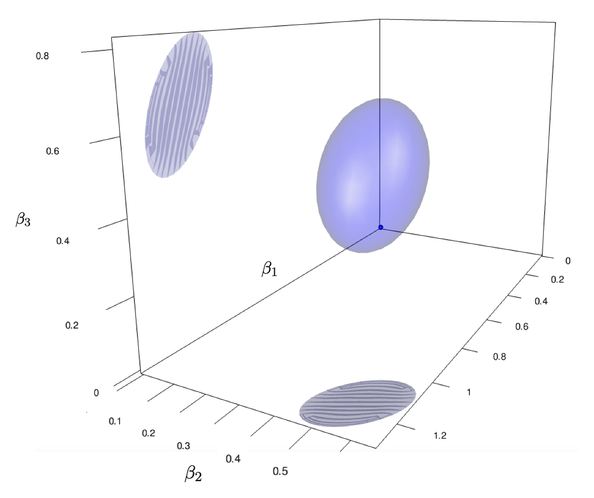
(a) (b)
F.4 Simulation result for an additional setting
Here we conduct a simulation study on Scenario (f) of the simulation conducted by [38] to demonstrate the performance of the propose repro samples approach in the low-dimensional setting when This simulation setting is as follows.
- (MA)
(From [38], with many signals) Let the true values For , the correlation between and is set to . We let and .
| Method | Cardinality of | Inclusion of | |
|---|---|---|---|
| Model MA: | Repro samples | 1.010 (0.007) | 1.000 (0.000) |
| Bootstrap AIC | 601.645 (12.612) | 1.000 (0.000) | |
| Bootstrap BIC | 246.995 ( 4.404) | 1.000 (0.000) | |
| Bootstrap CV | 567.150 (12.446) | 1.000 (0.000) |
| Method | Cardinality of | Coverage of | |
|---|---|---|---|
| Model MA: | Repro samples | 1.010 (0.007) | 1.000 (0.000) |
| Bootstrap AIC | 601.645 (12.612) | 1.000 (0.000) | |
| Bootstrap BIC | 246.995 ( 4.404) | 1.000 (0.000) | |
| Bootstrap CV | 567.150 (12.446) | 1.000 (0.000) |
Table 6 and Table 7 summarize the results for the candidate set and the 95% model confidence set respectively from simulation repetitions. The comparison of the proposed repro samples approach with the bootstrap is similar to those from (M1)-(M5) in Section 5.1. Even in this low-dimensional settings, the bootstrap approach would produce an excessive large amount of models (between 250 and 600), while our repro samples approach only needs about 1 model, smaller than reported for the (M4) setting in Table 2 as expected (since sample size is twice of ). This performance appears to be notably more efficient than the confidence bound approach reported in [38] for this Scenario (f): Figure 3 (f) of [38] indicates that the confidence bound needs to encompass at least 50 variables (about 25% of all variables). The reliance of their confidence bounds approach on bootstrap techniques, which generate a large number of models as indicated in Table 6 and Table 7 may have contributed partly to the excessively broad confidence bounds.
| Repro Samples | Debiased Lasso (JM) | Debiased Lasso (ZZ) | |||||
| Model | Coverage | Width | Coverage | Width | Coverage | Width | |
| MA | All | 0.998(0.000) | 0.018(0.000) | 0.971(0.001) | 0.320(0.000) | 0.964(0.001) | 0.339(0.000) |
| 0.960(0.004) | 0.296(0.000) | 0.950(0.004) | 0.319(0.001) | 0.959(0.004) | 0.338(0.000) | ||
| 1.000(0.000) | 0.000(0.000) | 0.973(0.001) | 0.320(0.000) | 0.965(0.001) | 0.339(0.000) | ||
| Repro Samples | Debiased Lasso (JM) | Debiased Lasso (ZZ) | ||||
|---|---|---|---|---|---|---|
| Coverage | Width | Coverage | Width | Coverage | Width | |
| 0.940(0.017) | 0.268(0.001) | 0.935(0.017) | 0.294(0.002) | 0.955(0.015) | 0.323(0.001) | |
| 0.970(0.012) | 0.300(0.001) | 0.940(0.017) | 0.320(0.002) | 0.945(0.016) | 0.338(0.001) | |
| 0.955(0.015) | 0.302(0.001) | 0.930(0.018) | 0.322(0.002) | 0.935(0.017) | 0.340(0.001) | |
| 0.960(0.014) | 0.301(0.001) | 0.955(0.015) | 0.320(0.002) | 0.955(0.015) | 0.339(0.001) | |
| 0.950(0.015) | 0.303(0.001) | 0.960(0.014) | 0.322(0.002) | 0.970(0.012) | 0.341(0.001) | |
| 0.945(0.016) | 0.300(0.001) | 0.960(0.014) | 0.320(0.002) | 0.955(0.015) | 0.339(0.001) | |
| 0.965(0.013) | 0.300(0.001) | 0.945(0.016) | 0.320(0.002) | 0.965(0.013) | 0.338(0.001) | |
| 0.960(0.014) | 0.300(0.001) | 0.945(0.016) | 0.319(0.002) | 0.960(0.014) | 0.338(0.001) | |
| 0.965(0.013) | 0.300(0.001) | 0.960(0.014) | 0.321(0.002) | 0.960(0.014) | 0.339(0.001) | |
| 0.980(0.010) | 0.302(0.001) | 0.975(0.011) | 0.322(0.002) | 0.980(0.010) | 0.341(0.001) | |
| 0.975(0.011) | 0.301(0.001) | 0.960(0.014) | 0.321(0.002) | 0.970(0.012) | 0.340(0.001) | |
| 0.950(0.015) | 0.269(0.001) | 0.940(0.017) | 0.322(0.002) | 0.955(0.015) | 0.340(0.001) | |
We summarized the performance of the repro samples confidence intervals for the regression coefficients along with those of the debiased confidence intervals in Table 8 and Table 9. In general, both the repro samples approach and the debiased methods achieve the desired coverage rates. However, proposed repro samples interval are significantly narrower compared to the debiased confidence intervals. In particular, the average length of our repro samples confidence interval is only about 6% of width of the debiased confidence intervals on average, mainly due to the advantage in the widths of the confidence intervals for the coefficients whose true values are 0’s. Even for the signals, we observe from Table 9 our repro samples approach consistently produces narrower confidence intervals compared to both of the debiased approaches for every single non-zero coefficients, while obtaining the desired coverage rate.
F.5 Simulation results for confidence sets of each nonzero coefficient.
| Repro Samples | Debiased Lasso (JM) | Debiased Lasso (ZZ) | |||||
| Model | Coverage | Width | Coverage | Width | Coverage | Width | |
| M1 | 0.970(0.012) | 0.714(0.008) | 0.310(0.033) | 0.244(0.008) | 0.990(0.007) | 1.266(0.014) | |
| 0.960(0.014) | 0.810(0.010) | 0.440(0.035) | 0.249(0.009) | 0.980(0.010) | 1.346(0.017) | ||
| 0.925(0.019) | 0.718(0.009) | 0.320(0.033) | 0.250(0.009) | 0.975(0.011) | 1.352(0.016) | ||
| M2 | 0.990(0.007) | 0.540(0.006) | 0.960(0.014) | 0.498(0.004) | 0.995(0.005) | 0.942(0.009) | |
| 0.965(0.013) | 0.544(0.006) | 0.915(0.020) | 0.498(0.005) | 0.980(0.010) | 0.941(0.010) | ||
| 0.965(0.013) | 0.538(0.007) | 0.935(0.017) | 0.494(0.005) | 0.995(0.005) | 0.936(0.010) | ||
| 0.980(0.010) | 0.540(0.006) | 0.930(0.018) | 0.494(0.004) | 0.990(0.007) | 0.933(0.009) | ||
| 0.975(0.011) | 0.533(0.007) | 0.950(0.015) | 0.499(0.004) | 0.985(0.009) | 0.946(0.009) | ||
| M3 | 0.980(0.010) | 0.458(0.005) | 0.870(0.024) | 0.427(0.003) | 0.995(0.005) | 0.942(0.010) | |
| 0.950(0.015) | 0.463(0.005) | 0.870(0.024) | 0.428(0.003) | 0.955(0.015) | 0.941(0.009) | ||
| 0.965(0.013) | 0.461(0.005) | 0.865(0.024) | 0.427(0.004) | 0.980(0.010) | 0.941(0.010) | ||
| 0.960(0.014) | 0.465(0.005) | 0.850(0.025) | 0.431(0.004) | 0.975(0.011) | 0.951(0.010) | ||
| 0.945(0.016) | 0.471(0.006) | 0.890(0.022) | 0.431(0.003) | 0.960(0.014) | 0.950(0.009) | ||
| 0.955(0.015) | 0.436(0.005) | 0.865(0.024) | 0.424(0.003) | 0.995(0.005) | 0.930(0.009) | ||
| M4 | 0.965(0.013) | 0.399(0.003) | 0.940(0.017) | 0.416(0.003) | 0.965(0.013) | 0.498(0.003) | |
| M5 | 0.970(0.012) | 0.723(0.009) | 0.255(0.031) | 0.243(0.009) | NA | NA | |
| 0.965(0.013) | 0.813(0.010) | 0.455(0.035) | 0.249(0.009) | NA | NA | ||
| 0.925(0.019) | 0.728(0.010) | 0.300(0.032) | 0.247(0.009) | NA | NA | ||
To further investigate the performance differences between the proposed approach and the two debiased Lasso methods, we compare in Table 10 the coverage rates and widths of the confidence sets for each nonzero regression coefficient. To save space, we only display the results of the confidence sets for of (M4) due to the similarity of the results across the 12 non-zero coefficients. Both the repro samples approach and debiased Lasso (ZZ) achieve the desired coverage regardless of the signal strengths, with the debiased Lasso (ZZ) intervals at least 70% wider. Conversely, the debiased Lasso (JM) uniformly undercovers the truths for all signals in all models except for the two coefficients in (M2). As expected, the under-coverage issue of the debiased Lasso (JM) approach is more serious when is larger, since the second order approximation is more difficult. For (M1) and (M5) with , the coverage rate of the debiased Lasso (JM) is only around 25%–45%, and for Model (M3) with the coverage rate is around 85%–89%. In terms of the width of the confidence sets, for Model (M3) with , the widths of the repro samples confidence sets are less than half of those from the debiased Lasso (ZZ) and comparable to the debiased Lasso (JM), which undercovers all the signals in (M3). For the other three models, the repro samples confidence sets are also at least 40% shorter than the debiased Lasso (ZZ) confidence intervals for the signals, providing a more accurate assessment of the uncertainties of the estimation of these regression parameters. To sum up, the repro samples approach covers all the signals with the desired coverage rate and correctly quantifies the uncertainty of parameter estimation regardless of the dimension of the design matrix and signal strength.