Data-Driven Stochastic Optimal Control Using Kernel Gradients Thanks: This material is based upon work supported by the National Science Foundation under NSF Grant Number CNS-1836900. Any opinions, findings, and conclusions or recommendations expressed in this material are those of the authors and do not necessarily reflect the views of the National Science Foundation. The NASA University Leadership initiative (Grant #80NSSC20M0163) provided funds to assist the authors with their research, but this article solely reflects the opinions and conclusions of its authors and not any NASA entity. Thanks: A. Thorpe, J. Gonzales, and M. Oishi are with Electrical & Computer Engineering, University of New Mexico, Albuquerque, NM. Email: {ajthor,jakegonzales,oishi}@unm.edu.

Let $(\mathcal{X},\mathscr{B}_{\mathcal{X}})$ be a Borel space called the state space and $(\mathcal{U},\mathscr{B}_{\mathcal{U}})$ be a compact Borel space called the control space. Consider a discrete-time stochastic system,

where $x_{t}\in\mathcal{X}\subseteq\mathbb{R}^{n}$, $u_{t}\in\mathcal{U}\subset\mathbb{R}^{m}$, and $w_{t}$ are independent and identically distributed (i.i.d.) random variables representing a stochastic disturbance. As shown in [15], the dynamics in (1) can equivalently be represented by a stochastic kernel $Q:\mathscr{B}_{\mathcal{X}}\times\mathcal{X}\times\mathcal{U}\to[0,1]$ that assigns a probability measure $Q(\cdot\mid x,u)$ on $(\mathcal{X},\mathscr{B}_{\mathcal{X}})$ to every $(x,u)\in\mathcal{X}\times\mathcal{U}$.

The system evolves from an initial condition $x_{0}\in\mathcal{X}$ (which may be drawn from an initial distribution $\mathbb{P}_{0}$ on $\mathcal{X}$) over a finite time horizon $t=0,1,\ldots,N$, $N\in\mathbb{N}$.

Let $g:\mathcal{X}\to\mathbb{R}$ be an arbitrary convex cost function, which we assume is measurable and bounded and lies in a Hilbert space of functions $\mathscr{H}$. At each time step, we seek the control $u\in\mathcal{U}$ that minimizes the following objective,

We assume that the stochastic kernel $Q$ is unknown, meaning we do not have direct information of the dynamics in (1) or the structure of the stochastic disturbance. Instead, we assume that we have access to a sample $\mathcal{S}=\{(x_{i},u_{i},y_{i})\}_{i=1}^{M}$ of observations taken i.i.d. from $Q$, where $x_{i}$ and $u_{i}$ are taken randomly from $\mathcal{X}$ and $\mathcal{U}$ and $y_{i}\sim Q(\cdot\mid x_{i},u_{i})$.

Because the stochastic kernel $Q$ is unknown, we cannot solve (2) directly since the integral in (2) is intractable. Instead, as shown in [9], we can use $\mathcal{S}$ to approximate the intractable integral with respect to $Q$ in (2) as an empirical embedding in a high-dimensional space of functions known as a reproducing kernel Hilbert space. Then, we can solve an approximation of the original problem in (2) in order to compute an approximately optimal control. We outline the procedure below, but refer the reader to [9] for more details.

Define a positive definite kernel function $k:\mathcal{X}\times\mathcal{X}\to\mathbb{R}$ [16, Definition 4.15]. According to the Moore-Aronszajn theorem [17], given a positive definite kernel $k$, there exists a unique corresponding reproducing kernel Hilbert space (RKHS) $\mathscr{H}$ with $k$ as its reproducing kernel.

Similarly, we define the RKHS $\mathscr{U}$ of functions from $\mathcal{U}$ to $\mathbb{R}$ with $l:\mathcal{U}\times\mathcal{U}\to\mathbb{R}$ as its associated reproducing kernel.

According to [1, 18], assuming the kernel $k$ is measurable and bounded, and given a probability measure $Q(\cdot\mid x,u)$, then by the Riesz representation theorem there exists a corresponding element $m(x,u)\in\mathscr{H}$ called the kernel distribution embedding, such that by the reproducing property, $\langle g,m(x,u)\rangle_{\mathscr{H}}=\int_{\mathcal{X}}g(y)Q(\mathrm{d}y\mid x,u)$. This means that by representing the integral operator with respect to $Q$ as an element in the RKHS, we can compute the expectation of any function $f\in\mathscr{H}$ as an RKHS inner product.

Using a sample $\mathcal{S}$, we can compute an empirical estimate $\hat{m}(x,u)$ of $m(x,u)$ as the solution to a regularized least-squares problem [18]. The solution is given by,

where $\Phi,\Psi$ are feature vectors with elements $\Phi_{i}=k(y_{i},\cdot)$ and $\Psi_{i}=k(x_{i},\cdot)l(u_{i},\cdot)$, respectively, and $G\in\mathbb{R}^{M\times M}$ is a real matrix where the $ij^{\rm th}$ element is $k(x_{i},x_{j})l(u_{i},u_{j})$. For simplicity of notation, let $W=(G+\lambda MI)^{-1}$.

Using the estimate $\hat{m}(x,u)$, we can approximate the intractable integrals with respect to $Q$ in (2) via an RKHS inner product,

where $\boldsymbol{g}$ is a vector with elements $\boldsymbol{g}_{i}=g(y_{i})$.

This representation is key to our approach, since it means we can approximate the previously intractable problem in (2) using data comprised of system observations.

Following [9], we can approximate the stochastic optimal control problem (2) using the estimate $\hat{m}(x,u)$ and (5) as,

Theoretically, we could optimize for $u$ directly. However, this is a non-convex problem in general, which makes solving (6) difficult. For example, it may be exceptionally difficult to solve (6) for common kernel choices such as the Gaussian kernel function, since optimizing a linear combination of Gaussians is a non-convex problem. Thus, finding a control action $u\in\mathcal{U}$ that minimizes the approximate problem presents a significant challenge.

One possible approach is given in [9, 10], where a stochastic control policy with finite support is represented as an embedding in the RKHS $\mathscr{U}$. Then, the policy can be obtained as the solution to a linear program, giving a set of probability values over a user-specified set of admissible control actions $\mathcal{A}\subset\mathcal{U}$. However, a significant drawback of this approach is the need to strategically select $\mathcal{A}$ such that it contains controls which are close to the true solution, and typically only finds a sub-optimal solution to the approximate problem.

We propose to compute the control input via a kernel-based stochastic gradient descent method. Using the properties of reproducing kernel Hilbert spaces, we can compute the gradient by taking the partial derivative of the kernel, rather than explicitly computing the gradient with respect to $u$. This allows us to optimize the control input by directly optimizing within the RKHS and avoids the problem of non-convexity in optimizing for $u$ in the approximate problem. An illustration of this idea is depicted in Figure 1.

Initializing the gradient descent algorithm close to the true solution ensures that we obtain an approximately optimal solution in fewer gradient steps. One possibility is to compute a sub-optimal initial guess for Algorithm 1 using [9].

As shown in [9], we can compute a solution to the (unconstrained) approximate stochastic optimal control problem in (6) by representing a stochastic policy $\pi:\mathscr{B}_{\mathcal{U}}\times\mathcal{X}\to[0,1]$ as a kernel embedding $p$ in the RKHS $\mathscr{U}$,

where $\gamma(x)\in\mathbb{R}^{P}$ are real-valued coefficients that depend on the state $x\in\mathcal{X}$, $\Upsilon$ is a feature vector with elements $\Upsilon_{j}=l(\tilde{u}_{j},\cdot)$, and the points $\mathcal{A}=\{\tilde{u}_{j}\}_{j=1}^{P}$ are a set of user-specified admissible control actions that we want to optimize over. The problem then becomes finding the coefficients $\gamma(x)$ that optimize the approximate control problem. According to [9], we can view the coefficients $\gamma(x)$ as a set of probabilities that weight the user-specified control actions in $\mathcal{A}$, which we can find as the solution to a linear program,

The linear program can efficiently be solved via the Lagrangian dual. Letting $C(x)=\boldsymbol{g}^{\top}W\Psi k(x,\cdot)\Upsilon^{\top}$, the solution according to [19] is given by a vector of all zeros except at the index $j=\arg\min_{i}\{C_{i}(x)^{\top}\}$, where it is $1$. In other words, we choose the control action in $\mathcal{A}$ that corresponds to the index $j$ which is the solution to the Lagrangian dual problem. See [9] for more details.

By choosing control actions in $\mathcal{A}$ that are good candidate solutions to the optimal control problem in (2), we obtain a good initial guess for the gradient-based learning algorithm. However, unlike the approach in [9], we do not require the approximately optimal solution to lie within $\mathcal{A}$, and we further improve the solution of the LP using stochastic gradient descent.

We consider the problem of regulation for a 2D stochastic chain of integrators system, with dynamics given by

where $x_{t}\in\mathbb{R}^{2}$ is the state, $u_{t}\in\mathbb{R}$ is the control input, which we constrain to be within $[-1,1]$, $w_{t}$ is a random variable with distribution $\mathcal{N}(0,0.01I)$, and $T_{s}$ is the sampling time. We seek to compute a control input $u$ as the solution to the following stochastic optimal control problem,

where $Q$ is a representation of the dynamics as a stochastic kernel. We use the cost function $g(x)=\lVert x\rVert_{2}$, which serves to drive the system to the origin.

We consider a sample $\mathcal{S}=\{(x_{i},u_{i},y_{i})\}_{i=1}^{M}$ of size $M=1600$ taken i.i.d. from $Q$. The states $x_{i}$ were taken uniformly in the region $[-1,1]\times[-1,1]$, the control inputs $u_{i}$ were taken uniformly from $[-1,1]$, and the resulting states were generated according to $y_{i}\sim Q(\cdot\mid x_{i},u_{i})$. We then presumed no knowledge of the system dynamics or the stochastic disturbance for the purpose of computing the approximately optimal control action using our proposed method. Using the sample $\mathcal{S}$, we then computed an estimate $\hat{m}$ of the kernel embedding $m$ as in (3) using Gaussian kernels with bandwidth parameter $\sigma=3$, chosen via cross-validation. We then selected $R=121$ evaluation points $\{x_{j}\}_{j=1}^{R}$ spaced uniformly in the region $[-1,1]\times[-1,1]$, from which to compute the optimal control actions.

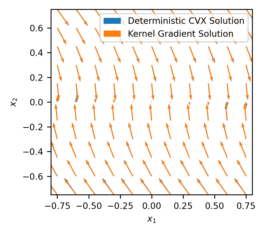
To provide a basis for comparison, we computed the optimal control actions using CVX from the evaluation points $\{x_{j}\}_{j=1}^{R}$ using the deterministic dynamics. We then propagate the dynamics forward in time using the optimal inputs to obtain the state at the next time instant. The vector field of the closed-loop dynamics under the optimal control inputs is shown in Figure 2 (blue). We then computed the approximately optimal control actions using Algorithm 1 with the sample $\mathcal{S}$ taken from the stochastic dynamics to minimize the cost at each point $\{x_{j}\}_{j=1}^{R}$ over a single time step. For Algorithm 1, we used a step size of $\eta=0.01$ and limited the number of iterations to $100$. The vector field of the closed-loop dynamics using the approximately optimal solution computed using our proposed method is shown in Figure 2 (orange).

We can see that the gradient based algorithm computes approximately optimal control inputs which closely match the solution computed via CVX. This demonstrates the effectiveness of the gradient-based algorithm to compute approximately optimal control actions with no prior knowledge of the dynamics or the stochastic disturbance.

Note that the quality of the empirical approximation of the cost surface depends on the sample size $M$. As the sample size increases, the approximation improves, and we obtain a closer approximation of the optimal solution using our method. To demonstrate this, we computed the mean error and the maximum error between the data-driven gradient-based solution and the solution via CVX using the deterministic dynamics for varying sample sizes $M\in[250,2500]$ averaged over $20$ iterations. The results are shown in Figure 3. We can see that the error of the approximately optimal solution decreases as $M$ increases. However, we can also see that the quality of the solution does not improve appreciably as the sample size increases, which is due to the asymptotic convergence of the estimate $\hat{m}$ to the true embedding $m$. This presents a tradeoff between computation time and numerical accuracy, since the computational complexity scales polynomially with the sample size.

We consider the problem of target tracking for a nonholonomic vehicle system as in [9]. The dynamics are given by

where $x=[x_{1},x_{2},x_{3}]^{\top}\in\mathbb{R}^{3}$ are the states, $u=[u_{1},u_{2}]^{\top}\in\mathbb{R}^{2}$ are the control inputs. The control inputs are constrained such that $u_{t}\in[0.5,1.2]\times[-10.1,10.1]$. We discretize the dynamics in time using a zero-order input hold and apply an affine disturbance $w\sim\mathcal{N}(0,0.01I)$. We define a target trajectory as a sequence of position coordinates indexed by time, shown in Figure 4 (blue). We choose an initial condition of $x_{0}=[-1,-0.2,\pi/2]^{\top}$, and evolve the system forward in time over the time horizon $N=20$. At each time $t$, starting at $t=0$, we seek to compute a control input $u_{t}$ as the solution to the following stochastic optimal control problem,

where the cost function $g_{t}(x)$ seeks to minimize the squared Euclidean distance of the system’s position to the target trajectory’s position at each time step.

We consider a sample $\mathcal{S}=\{(x_{i},u_{i},y_{i})\}_{i=1}^{M}$, with sample size $M=3000$. The states $x_{i}$ were taken uniformly within the region $[-1.2,1.2]\times[-1.2,1.2]\times[-\pi,\pi]$, the control actions $u_{i}$ were taken uniformly within the region $[0.5,1.2]\times[-10.1,10.1]$, and the resulting states were drawn according to $y_{i}\sim Q(\cdot\mid x_{i},u_{i})$. Using the sample $\mathcal{S}$, we then computed an estimate $\hat{m}$ of the kernel embedding $m$ as in (3) using Gaussian kernels with bandwidth parameter $\sigma=3$, chosen via cross-validation.

In order to compute a baseline for comparison, we then computed the control actions using [9], which computes a stochastic policy embedding $p_{t}$ at every time step over a finite set $\mathcal{A}=\{\tilde{u}_{j}\}_{j=1}^{210}$, as in (12). We chose the controls $\tilde{u}_{j}$ in the admissible set $\mathcal{A}$ to be uniformly spaced in the range $\tilde{u}_{j}\in[0.5,1.2]\times[-10.1,10.1]$. Starting at the initial condition $x_{0}$, we then computed the control actions by solving (13) at each time step forward in time. The resulting trajectory is plotted in Figure 4 (green), had a total cost of $\sum_{t=0}^{N}g_{t}(x_{t})=1.447$, and the computation time was $1.159$ seconds.

We then evolve the system forward in time using the approximately optimal control action selected via the kernel-based gradient descent algorithm (Algorithm 1), and initializing using the solution to (13) using $\mathcal{A}$ as above. For Algorithm 1, we chose a step size of $\eta=0.1$ and limited the number of gradient iterations to $100$. The resulting trajectory is plotted in Figure 4 (orange), and has a total cost of $\sum_{t=0}^{N}g_{t}(x_{t})=1.363$. The total computation time was $8.865$ seconds. As expected, we see that the trajectory computed using our method more closely follows the target trajectory (has a lower overall cost). This shows that the gradient-based algorithm is able to compute the approximately optimal control actions for a nonlinear system at each time step, using only data collected from system observations.

References

- [1] L. Song, J. Huang, A. Smola, and K. Fukumizu, “Hilbert space embeddings of conditional distributions with applications to dynamical systems,” in Int’l Conf. Mach. Learn., 2009, p. 961–968.
- [2] S. Grünewälder, G. Lever, L. Baldassarre, M. Pontil, and A. Gretton, “Modelling transition dynamics in MDPs with RKHS embeddings,” in Int’l Conf. Mach. Learn., 2012, p. 1603–1610.
- [3] Y. Nishiyama, A. Boularias, A. Gretton, and K. Fukumizu, “Hilbert space embeddings of POMDPs,” in Conf. Uncertainty in Artificial Intelligence, 2012, p. 644–653.
- [4] G. Lever and R. Stafford, “Modelling policies in MDPs in reproducing kernel Hilbert space,” in Int’l Conf. Artificial Intelligence and Statistics, vol. 38, 2015, pp. 590–598.
- [5] N. A. Vien, P. Englert, and M. Toussaint, “Policy search in reproducing kernel Hilbert space,” in Int’l Joint Conf. on Artificial Intelligence, 2016, p. 2089–2096.
- [6] L. Song, B. Boots, S. M. Siddiqi, G. Gordon, and A. Smola, “Hilbert space embeddings of hidden Markov models,” in Int’l Conf. Mach. Learn. Madison, WI, USA: Omnipress, 2010, p. 991–998.
- [7] L. Song, K. Fukumizu, and A. Gretton, “Kernel embeddings of conditional distributions: A unified kernel framework for nonparametric inference in graphical models,” IEEE Signal Process. Mag., vol. 30, no. 4, pp. 98–111, 2013.
- [8] K. Fukumizu, L. Song, and A. Gretton, “Kernel Bayes’ rule: Bayesian inference with positive definite kernels,” J. Mach. Learn. Res., vol. 14, no. 1, p. 3753–3783, dec 2013.
- [9] A. Thorpe and M. Oishi, “Stochastic optimal control via Hilbert space embeddings of distributions,” in IEEE Conf. Dec. & Ctrl., 2021, pp. 904–911.
- [10] A. Thorpe, T. Lew, M. Oishi, and M. Pavone, “Data-driven chance constrained control using kernel distribution embeddings,” in Learn. for Dynamics and Ctrl. Conf., vol. 168, 2022, pp. 790–802.
- [11] Y. Nemmour, H. Kremer, B. Schölkopf, and J.-J. Zhu, “Maximum mean discrepancy distributionally robust nonlinear chance-constrained optimization with finite-sample guarantee,” arXiv preprint arXiv:2204.11564, 2022.
- [12] Z. Li, D. Meunier, M. Mollenhauer, and A. Gretton, “Optimal rates for regularized conditional mean embedding learning,” arXiv preprint arXiv:2208.01711, 2022.
- [13] Z. Marinho, B. Boots, A. Dragan, A. Byravan, G. J. Gordon, and S. Srinivasa, “Functional gradient motion planning in reproducing kernel Hilbert spaces,” in Robotics: Science and Systems, 2016.
- [14] D.-X. Zhou, “Derivative reproducing properties for kernel methods in learning theory,” J. Computational and Applied Mathematics, vol. 220, no. 1-2, pp. 456–463, 2008.
- [15] D. Bertsekas and S. Shreve, Stochastic optimal control: the discrete-time case. Athena Scientific, 1978, vol. 5.
- [16] I. Steinwart and A. Christmann, Support Vector Machines. Springer Science & Business Media, 2008.
- [17] N. Aronszajn, “Theory of reproducing kernels,” Trans. of the American Mathematical Society, vol. 68, no. 3, pp. 337–404, 1950.
- [18] S. Grünewälder, G. Lever, L. Baldassarre, S. Patterson, A. Gretton, and M. Pontil, “Conditional mean embeddings as regressors,” in Int’l Conf. Mach. Learn., 2012, p. 1803–1810.
- [19] S. Boyd, S. P. Boyd, and L. Vandenberghe, Convex optimization. Cambridge university press, 2004.
- [20] A. Thorpe and M. Oishi, “SOCKS: A stochastic optimal control and reachability toolbox using kernel methods,” in Hybrid Syst.: Comput. and Ctrl., 2022.