Arrested development and fragmentation in Strongly-Interacting Floquet Systems
We explore how interactions can facilitate classical like dynamics in models with sequentially activated hopping. Specifically, we add local and short range interaction terms to the Hamiltonian, and ask for conditions ensuring the evolution acts as a permutation on initial local number Fock states. We show that at certain values of hopping and interactions, determined by a set of Diophantine equations, such evolution can be realized. When only a subset of the Diophantine equations is satisfied the Hilbert space can be fragmented into frozen states, states obeying cellular automata like evolution and subspaces where evolution mixes Fock states and is associated with eigenstates exhibiting high entanglement entropy and level repulsion.
Keywords:
Interactions, Floquet, ThermalizationI Introduction
As experimental tools have progressed (e.g. Bloch2008Ultracold; Blatt2012TrappedIon), the microscopic control of quantum systems has become increasingly accessible. These advancements, along with a correlated increase in theoretical interest, have led to the discovery of many new and surprising phenomena that emerge when periodic driving, interactions, and their interplay are considered.
For example, periodically driven systems can be used to stabilize otherwise unusual behavior. A recent important example is topological Floquet insulators Kitagawa2010FTI; lindner2011Floquet; Rudner2020FTI, where novel topological features of the band structure may emerge due to inherent periodicity of the non-interacting quasi- energy spectrum. Furthermore, it was shown in titum2016anomalous that, by combining spatial disorder with a topological Floquet insulator model introduced by Rudner-Lindner-Berg-Levin (RLBL) rudner2013anomalous, a new topological phase may be realized called the anomalous Floquet-Anderson insulator (AFAI). Discrete time crystals Sacha2020DTCBook; Else2020DTCRev; Khemani2016DTC; Else2016DTC are another important example of behavior that may occur in periodically driven, but not static Watanabe2015noTC, systems. Namely, a time crystal is a system where time-translation symmetry is spontaneously broken (in analogy to spatial translation symmetry spontaneously breaking to form ordinary crystals).
Combining periodic driving with interactions, however, can often be problematic as generic, clean, interacting Floquet system are expected to indefinitely absorb energy from their drive and thus quickly converge to a featureless infinite temperature state Lazarides2014Therm; Dalessio2014Therm; Ponte2015Therm. This problem may be side-stepped by considering Many-Body Localization (MBL) Abanin2019MBLRev; DAlessio2013MBL; Ponte2015MBL; Ponte2015MBLPRL; Lazarides2015MBL; Khemani2016MBL; Agarwala2017MBL, in which strong disorder is utilized to help stave off thermalization, by considering the effective evolution of pre-thermal states Bukov2015pretherm; Kuwahara2016pretherm; Else2017pretherm; Abanin2017pretherm; Zeng2017pretherm; Machado2019pretherm that, in the best cases, take exponentially long to thermalize, or by connecting the system to a bath to facilitate cooling and arrive at interesting, non- equilibrium steady-states Dehghani2014Dissipative; Iadecola2015Bath; Iadecola2015Bath2; Seetharam2015Bath.
Yet another route for realizing non-trivial dynamics despite the expected runaway heating from interacting, Floquet drives is to consider systems where the ergodicity is weakly broken, i.e. where there are subspaces (whose size scales only polynomially in the system size) of the Hilbert space that do not thermalize despite the fact that the rest of the Hilbert space does. These non-thermal states are called quantum many-body scars Turner2018Scars; Ho2019Scars; Moudgalya2022Scars and have been shown to support many interesting phenomena including, for example, discrete time crystals Yarloo2020ScarDTC. Furthermore, in constrained systems, the full Hilbert space may fragment into subspaces where some of the subspaces thermalize while others do not Sala2020HFrag; Moudgalya2022Scars. When the fraction of non-thermal states are a set of measure zero in the thermodynamic limit, the system is an example of quantum many-body scarring. However, in other cases, the non-thermal subspaces form a finite fraction of the full Hilbert space and therefore correspond to a distinct form of ergodicity breaking.
In addition to leading to heating, interactions are also often responsible for our inability to efficiently study or describe many body quantum states in both Floquet and static Hamiltonian systems. However, there are situations when interactions play the opposite role in creating specialized states of particular simplicity or utility. For example, systems with interactions can exhibit counter-intuitive bound states due to coherent blocking of evolution. A nice class of such systems are the edge-locked few particle systems studied in haque:060401; haque2010self.
In this work, we consider Floquet drives where hopping between neighboring pairs of sites are sequentially activated. The theoretical and experimental tractability of such models have made them a popular workhorse for fleshing out a broad range of the exciting properties of periodically driven systems (e.g. rudner2013anomalous; Kumar2018evenodd; Ljubotina2019evenodd; Piroli2020evenodd; Lu2022EvenOddPRL). We find that, when interactions are added to such systems, there exist special values of interaction strength and driving frequency where the dynamics becomes exactly solvable. Furthermore, the complete set of these special parameter values may be determined via emergent Diophantine equations Cohen2007Dioph. At other parameter values, the Hilbert space is fragmented. Initial states contained within some, thermal, subspaces will ergodically explore the subspace (though not the entire Hilbert space), while other initial states contained within other, non-thermal, subspaces will evolve according to a classical cellular automation (CA) Wolfram1983CA, i.e. the system evolves in discrete time steps where after each step the occupancy of any given site is updated deterministically based on a small set of rules determined by the occupancy of neighboring sites.
As examples, we consider RLBL(-like) models with added nearest neighbor (NN) or Hubbard interactions as well as an even-odd Floquet drive in one dimension with NN interactions (more detailed descriptions of these models given below). We note that some work has been done in the first two cases Nathan2019AFI; Nathan2021AFI where it was argued that novel, MBL anomalous Floquet insulating phases emmerged when a disorder potential was added. We will discuss how our focus on special parameter values leads to new insights into these models and how it suggests a possible route towards other exciting phenomena such as the support of discrete time crystals within fragments of the Hilbert space.
II Conditions for evolution by Fock state permutations
In this section, we examine conditions for deterministic evolution of Fock states into Fock states in fermion models. Here we consider real space Fock states, which have a well defined fermion occupation on each lattice site (We will also refer to such states as fermion product states). We consider models where hopping between non-overlapping selected pairs of sites is sequentially activated. Two models of this type, discussed in detail below, deal with Hubbard and nearest neighbour interactions. The approach can be naturally extended to deal with more general interactions in sequentially applied evolution models.
II.1 Example 1: Hubbard-RLBL
As a particularly illuminating example, consider the Rudner-Lindner-Berg-Levin model rudner2013anomalous. This model is an exact toy model for a topological Floquet insulator and has been very useful in flushing out some of their salient properties. In addition, it provides the starting point for other states, such as the anomalous Floquet-Anderson insulators titum2016anomalous. The model is two dimensional, however, it’s simplicity lies in its similarity to even-odd type models, Kumar2018evenodd; Ljubotina2019evenodd; Piroli2020evenodd; Lu2022EvenOddPRL, in that the evolution activates disjoint pairs of sites at each stage. The model can be tuned to a particular point where the stroboscopic evolution of product states is deterministic exhibiting bulk periodic motion and edge propagation. Similarly, one can tune the driving frequency to completely freeze the stroboscopic evolution. Here, we add interactions to the model and ask when we can make the evolution a product state permutation, at least in some sectors. The Hubbard-RLBL evolution is written as
| (1) |
where . For ,
| (2) |
where and the sets are described in Fig. 1.
Note, this is equivalent to the model investigated in Nathan2021AFI when , i.e. the waiting period corresponds to evolution with random local potentials and no hopping 11 1 Technically, in Nathan2021AFI a weak disorder potential is added during the steps and then the disorder strength during the wait step is effectively made stronger by increasing the length of time the wait step is applied. However, this slight difference in how the disorder potential is applied does not seriously alter the dynamics and so we will not make a hard distinction between the two.. In that work, it was shown that this model supports a new family of few-body topological phases characterized by a hierarchy of topological invariants. These results may be viewed from the following perspective. First, finely-tuned points where the dynamics is exactly solvable were studied (namely, and or ). Second, it is argued that regions near these special points are stabilized (i.e. localized, at least for finite particle number cases) by disorder leading to robust phases. Finally, topological invariants characterizing these phases (V small vs. V large) can be found and shown to be distinct implying two differing topological phases. An application of the methods we propose in this work will allow us to generalize the first step above and find families of these exactly solvable points. We leave discussions of when regions in parameter space near these points may or may not be stabilized by disorder to future work. Since, at these exactly solvable points, we will be mapping product states to product states, will only act as an unobservable global phase and thus for the rest of our analysis we will set . Furthermore, throughout the rest of the paper we will work in units where and .

We now look for conditions to simplify the evolution (1) in such a way that the total evolution reduces to a permutation on the set of product states, i.e. when an initial configuration of fermions is placed at a selection of locations it will evolve into a different assignment of locations without generating entanglement.
To do so, we note that the evolution of each pair of sites, may be considered separately due to the disjoint nature of the set of pairs . Thus, we consider the evolution on a pair of sites
| (3) |
Since the evolution preserves particle number, we can treat the sub-spaces of and particles in each neighboring pair of sites separately. In the case of or particles, evolution is trivially the identity (due to Pauli blocking in the particle case). For or particles, one of the two sites is always doubly occupied, and thus the interaction term in (2) is a constant and does not affect evolution. In this case, solving the two site non-interacting evolution we see that in the one-particle sector, a fermion starting initially at site has a probability to hop to the other site in pair and probability to stay. Similarly, in the 3-particle sector, an initially placed hole in site has the same probability, to hop to the other site . Thus, when
| (4) |
for some integer , evolution for initial product states in the , particle subspace is completely deterministic with trivial evolution for even and the particle hopping to the other site in the pair with probability (henceforth referred to as perfect swapping) when is odd. Clearly, for these values of (and independently of ), no new entanglement is created in any pairs with or particles. To render the evolution in the particle pair subspace simple, it is shown in appendix A.1 that deterministic evolution occurs when the two conditions below are simultaneously satisfied:
| (5) | |||
| and | |||
| (6) |
with . Note that (5) guarantees the preservation of the number of doubly occupied sites (doublons). When is even, the sub-system will return to its initial state. On the other hand, if is odd, the system will exhibit perfect swapping i.e. each particle will hop to the other site in the pair. By solving for and in terms of and , we may now summarize when evolution is deterministic in each of the particle number sub-spaces:
|
when or are even (odd) evolution is frozen (perfect swapping). To keep the solutions real, Eq. II.1 also implies we must take .
II.2 The Diophantine Equation
Combining the conditions (4), (5), and (6) together yields the following equation:
| (11) |
Eq. (11) is a homogeneous Diophantine equation of degree and can be solved.
We now give a brief review of Diophantine equations and the strategy for solving homogenous quadratic equations.
Diophantine equations are algebraic (often polynomial) equations of several unknowns where only integer or rational solutions are of interest. They are named in honor of Diophantus of Alexandria for his famous treatise on the subject written in the 3rd century though the origins of Diophantine equations can be found across ancient Babylonian, Egyptian, Chinese, and Greek texts Cohen2007Dioph. Despite their often innocuous appearance, they are an active area of research with solutions frequently requiring surprisingly sophisticated mathematical techniques and have been the centerpiece of several famous, long-standing mathematical problems that have only been (relatively) recently resolved, including Fermat’s Last Theorem Wiles1995Fermat and Hilbert’s Tenth Problem Matiyasevich1970Hilbert.
In this section, we are interested in the relatively simple case of a homogeneous quadratic Diophantine equation, i.e. equation of the form
| (12) |
with variables and coefficients given by the symmetric matrix with integral diagonal entries and half integral off-diagonal entries. As we shall see, however, for interactions beyond Hubbard a broader class of Diophantine equations may need to be considered. For information on broader classes of Diophantine equations and for more information on the derivation to follow, see, for example, Cohen2007Dioph.
The general strategy for finding rational (we will specialize to integer solutions for our cases of interest at the end) solutions to (12) is to first find a particular solution and then generate all other rational solutions from the particular solution. Particular solutions can be found simply by inspection or through existing efficient algorithms Cohen2007Dioph. The main task is then to generate all other rational solutions from a given particular solution.
Take to be a particular solution, i.e.
| (13) |
Since (12) is quadratic, any line through will intersect the hypersurface defined by (12) at a single other point (see Fig. 2). Furthermore, if the line through is rational (i.e. has rational coefficients), as we see below, this implies that the second intersection point must also be rational. Therefore, it is possible to generate every rational solution to (12) by finding the second intersection point of every rational line through , where is rational.

Here, since (12) is homogeneous, it is convenient to work in projective space where a general line passing through is parameterized by
| (15) | |||
| (16) |
where we have simplified using (13). We may thus take as the solution . Combining with Eq (14) and multiplying by a general to restore full solutions (since we considered as an element of a projective space), we find
| (17) |
For integer solutions, we need simply to rescale and where . After rescaling, the only non-integer information is coming from , so all integer solutions may be found simply by considering integer .
For the relevant case of , let us, without loss of generality, diagonalize and let where (after rescaling with ) and are co-prime integers and the final element of may be set to due to the required linear independence with . Simplifying (17) then becomes
II.3 Solution for product state permutation dynamics with Hubbard interaction
Following the previous section, we write our Diophantine eq. (11) in a diagonal form:
| (27) | |||
where we have defined . Note, this is the famous Diophantine equation for Pythagorean triples.
By inspection, a non-trivial solution is . Utilizing Eq. (II.2) we find
Note, Eq. (II.3) is the standard solution for Pythagorean triples.
We thus found that the set of , , and simultaneously satisfying the conditions for simple dynamics can be written as:
| (47a) | |||
| (47b) | |||
| (47c) | |||
where and are coprime. Note, in (47), if is even (odd) then so is . This implies that the only way to completely satisfy the conditions in Eq. (II.1) is if all motion is frozen or all motion (not constrained by Pauli exclusion) becomes perfect swapping.
Inspecting the above solutions, we see that , automatically satisfying the condition for and to be real. Finally our solution is summarized by
| (48) |
Note that doesn’t depend on the choice of , and that any choice involving or will yield a non-interacting model.
As an illustration, consider the following example choices:
1. Taking yields , which is the non-interacting dynamics considered in the original RLBL model, with perfect swapping.
2. Taking yields . Since is even in this case, the dynamics is completely frozen.
3. Taking yields , i.e. frozen dynamics in a model with an attractive Hubbard interaction.
It is important to note that the special values of interaction strength and driving frequency in Eq. (48) hold for any Hubbard-Floquet procedure where hopping between pairs of sites is sequentially activated. This is the case for such systems on any lattice and in any dimension. We also note, that the Diophantine solution is ill suited to describe the singular case of infinite and finite and therefore this situation must be handled separately. In the limit of large , the interaction strength overpowers the hopping strength and all evolution is frozen in the 2-particle sector. On the other hand, evolution in the 1,3 particle sector is independent of and therefore may exhibit perfect swapping or freezing. Thus, in this case, it is possible to have one sector (the 2-particle sector) frozen while the other (the 1,3 particle sector) exhibits perfect swapping.
II.4 Example 2: Nearest neighbour interactions on a Lieb lattice.
In the next two examples, we consider interactions involving nearest neighbours. Unfortunately, adding nearest neighbour interactions to the RLBL model directly destroys an essential feature for the solvability of the problem: that the evolution operators of different pairs of sites are not directly coupled (and therefore commute). Here, instead, we choose to work with RLBL-like dynamics on a Lieb lattice as described in wampler2021stirring. The dynamics we consider here essentially activates pairs that are separated by several lattice sites at each step. The sequence of activations is described in Fig 3.

Here, we consider spinless fermions on the Lieb lattice. There are 8 steps. At step we activate hopping between sites that are nearest neighbours that belong to the set . The evolution is given by:
| (49) |
where , and
| (50) |
We proceed, as in Section II.1, by considering the evolution of a single connected pair during step and exactly solving for values of and where the pair exhibits freezing or perfect swapping. The evolution of a 2-site pair of sites for one step is given by
| (51) |
Note that the number operators on neighbours of commute with the evolution. Let the initial number of occupied neighbours of the sites and be and respectively (not counting themselves). Evolution of the 2-site pair is now exactly solvable in terms of , the difference in the number of particles neighboring sites and in the 2-site pair respectively (see Figure 4).
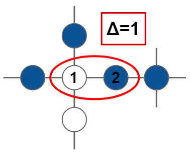
Solving the two site evolution, we find that evolution is frozen when
| (52) |
for some . We find that the evolution may only be perfect swapping when and occurs when for (see appendix A.2 for details).
In the rest of the paper, whenever considering the evolution on a pair of sites, we will denote as the difference in the number of (static) particles that are nearest neighbours of the two sites during the relevant evolution step.
II.5 A coupled set of Diophantine Equations
For a generic initial position of the particles, will not be uniform across the sample. Thus, for proper particle permutation dynamics, we must simultaneously find a solution of (52) for all possible values of .
Note that takes the values , where is the degree (number of neighbours) of lattice site . It follows that . Thus, if is the maximum degree of the lattice, we have the simultaneous conditions:
| (53) | |||
| (54) |
with all .
Equations (53) and (54) provide equations that must be solved simultaneously. The first two equations set the values for and in terms of , :
| (55) |
However, the rest of the equations for , with , must be simultaneously solved with these values for and yielding the coupled equations:
| (56) | |||
| (57) |
A first solution to this system may be obtained by taking , which, by (55), yields the non-interacting case . We now search for non-trivial solutions (i.e. ).
Solution for . For , we describe a general solution in appendix A.2 that yields non-trivial solutions. The result:
We note that is always even and thus all evolution is frozen. Due to the hierarchy of the equations, total freezing must then occur for any solutions with .
Solution for . We combine equations (II.5) and the equation from (53) to find a new Diophantine equation for the case :
| (64) |
The Diophantine equation (64) is harder to solve. However, a numerical search does find non-trivial () solutions. For example, is a solution with and . Whether there exist such that lattices with a maximum degree larger than may exhibit fully product state permutation evolution is an open question. The result for suggests the conjecture that there are solutions to the system of equations for any . Similar to the strategy above, by solving for , it is possible to construct a new Diophantine equation for . Determining whether this tower of equations is solvable is outside the scope of the present paper. On the other hand, as can already be seen in the case of , the values of for which the system exhibit such freezing for any initial number state quickly become prohibitively large for typical physical systems as the maximum lattice degree increases.
Remark. It is straightforward to generalize the Hamiltonian (50) to include more elaborate interactions as long as at each step the number operators associated with the neighbourhood of each evolving pair is constant. For example, we can write
| (65) |
Given the number of particles in the neighborhood of each 2-site pair, we write (note here we include the potentials in the the definition of ):
| (66) |
and the freezing condition becomes:
| (67) |
for all of the form (66).
II.6 Example 3: Deterministic evolution in the measurement induced chirality model on a Lieb lattice.
As another example, We consider the measurement induced chirality protocol of wampler2021stirring with added nearest neighbour interactions and in the Zeno limit. In that work, a simple hopping Lieb lattice model of fermions was subjected to repeated measurements changing according to a prescribed chiral protocol. In contrast to the previous models, the Hamiltonian is not time dependent and all hopping terms in the Hamiltonian remain activated throughout the process.
It was shown in wampler2021stirring that in the limit of rapid measurements, the so called the Zeno limit, the resulting dynamics is a classical stochastic process of permuting Fock states. We will see that, in this case too, we can find special values of interaction strength and protocol duration where the dynamics becomes deterministic. In fact, we will see the dynamics is governed by the same Diophantine equation as in example 2.
Specifically, we consider fermions hopping on a Lieb lattice with nearest-neighbor interactions given by
| (68) |
We now apply the measurement protocol introduced in wampler2021stirring to the system. Namely, we consider an 8 step measurement protocol in which, during the step that runs for a time , the local particle density in all sites in a set of sites are measured. In the Zeno limit, all evolution during a step is restricted to neighboring sites in the subspace (See figure 3 for details), while the rest of the sites are kept frozen. Thus, in the Zeno limit, the evolution is effectively split into steps evolved by the Hamiltonian (50), interspersed by an additional measurement. The measurements keep projecting the system onto Fock states, however, the particular states at hand are statistically distributed. However, if the step evolution (51) maps Fock states into Fock states, the whole procedure yields a deterministic evolution of an initial Fock state into another. In other words, the conditions for permutative evolution (and the corresponding set of Diophantine equations) for this model are equivalent to those found in the interacting Floquet model investigated in example 2.
III Hilbert Space Fragmentation
In Section II.5, we gave conditions that must be simultaneously satisfied for Fock state permutative dynamics in models on a Lieb lattice with NN interactions. Similarly, in Section II.1 we gave conditions for permutative evolution in the Floquet-Hubbard RLBL model. If in these models not all of these conditions are satisfied, then the evolution of a general initial state will require consideration of the full quantum many-body Floquet Hamiltonian.
However, evolution for certain initial states may still be deterministic even if only one or a few of the conditions for Fock state to Fock state evolution are met. This fragments Moudgalya2022Scars the Hilbert space, , into disconnected Krylov supspaces, , i.e.
| (69) |
where we have chosen a states that are number local states in such a way that are unique. In the rest of this section, we will explore the nature of the Hilbert space fragmentation in the example interacting Floquet and measurement induced models discussed in the previous section. Namely, we will see how the Hilbert spaces in these systems simultaneously support Krylov subspaces that are one-dimensional and correspond to frozen product states, few dimensional and correspond to states that evolve according to a classical cellular automation Wolfram1983CA, and exponentially large subspaces that may evolve with more generic quantum many-body evolution.
III.1 Arrested development
Let us take as an example the NN-RLBL model on a Lieb lattice considered in Section II.4. We have seen that satisfying the ith condition in equations (53) and (54) implies that evolution on any neighboring pair of sites will be frozen if (and also requiring is even if ). Thus, any given number state will be frozen under the evolution so long as every neighboring 2-site pair in the system containing a single particle has . In figure 5, we provide example frozen states for several values of .

Since these frozen states are trivially mapped back onto themselves (stroboscopically), they correspond to one-dimensional Krylov subspaces. Note, disjoint unions of frozen particle configurations will also be frozen. Therefore, since the number of possible disjoint unions of these frozen particle configurations grows exponentially with the system size, so too will the number of one-dimensional Krylov subspaces.
Furthermore, if several of the conditions (53) and (54) are satisfied, say the and conditions, then a zoo of frozen particle configurations emergres. Any disjoint unions of particle configurations satisfied by or alone will be satisfied. Additionally, new frozen particle configurations will emerge that simultaneously require both the and conditions to be frozen. An example particle configuration requiring the simultaneous satisfaction of the and condition is also given in Figure 5.
We emphasize here that the chiral nature of the Floquet procedure played no role in the emmergence of these frozen states. In fact, any procedure that sequentially activates hopping between neighboring pairs of sites (suitably spaced to keep evolution disjoint after adding NN interactions) will exhibit the exact same frozen states.
For example, consider a new procedure where, at each step in the evolution, the system is evolved with a from equation (49) chosen at random (uniformly), i.e. an example realization of this aperiodic, random evolution is given by
| (70) |
The exact same states will be frozen in this model as in the NN-RLBL model on a Lieb lattice and therefore the two models will share each of the one-dimensional Krylov subspaces. In the random model, the Hilbert space fragmentation will thus be split amongst an exponentially large number of one-dimensional, frozen, Krylov subspaces and a single Krylov subspace whose dimension scales exponentially with the system size. Due to the random, aperiodic nature of the full evolution, we expect evolution within the large-dimensional Krylov subspace to correspond to chaotic dynamics. In other words, we expect that time evolution of a random initial product state under (70) will result in either frozen evolution or ergodic dynamics within the Krylov subspace (for more on Krylov-restricted thermalization see Moudgalya2021scarbook). Both results will occur a finite fraction of the time depending on the initial product state.
III.2 Krylov Subspaces of Cellular Automation
Since the dynamics of a particle configuration that obey the Diophantine conditions depends crucially on particles on the neighbouring sites, it can be naturally encoded as a cellular automation step. We will now see how Krylov subspaces supporting classical CA Wolfram1983CA at each evolution step may emerge in interacting Floquet and measurement-induced systems when a few of the conditions for number state to number state evolution are satisfied.
To elucidate this effect, we consider again the NN-RLBL model on the Lieb lattice. In this case, we take the and the conditions for number state to number state evolution to both be satisfied, but this time the condition is satisfied for perfect swapping while the condition is satisfied for freezing. This may happen at, for example, and .
It is now possible to find number states such that the initial particle configuration, , and the resulting states after evolution of each step in the Floquet drive, all satisfy either or for every activated two-site pair in the system with a single particle. We give an example particle configuration where this may occur in Figure 6. Here, the space of states defines a Krylov subspace where evolution is completely given by a CA since at each step in the Floquet drive the local particle densities are updated deterministically based on the neighboring particle densities (i.e. if or ).

Similarly to the case of frozen initial particle configurations, disjoint unions of particle configurations that evolve as a CA will also evolve as a CA. For particle configurations whose CA evolution leaves all particles contained in a volume that does not scale with system size (for example, the evolution of the configuration in Figure 6 remains contained within the site square), the number of CA Krylov subspaces will grow exponentially with the system size (since there are exponentially many disjoint unions of such particle configurations). These CA subspaces may coexist with frozen Krylov subspaces as well as with exponentially large subspaces with more general quantum evolution.
It is important to note that these CA subspaces break the underlying time translation symmetry of the evolution operator. For example, the particle configuration in Fig. 6 returns to its initial configuration after . However, the exact realization of this Krylov subspace requires fine-tuning in parameter space. If an alteration of this model was possible such that the realization of these Krylov subspaces did not require fine-tuning, then such a model would be a realization of a time-crystal. In fact, since the systems we’ve considered may simultaneously support Krylov supspaces that break the time translation symmetry in different ways, such a stabilized system would simultaneously support several different time crystals depending on which Krylov subspace contains the initial state. Recent works Nathan2019AFI; Nathan2021AFI have argued that disorder may stabilize dynamics for regions in parameter space near similarly fine-tuned points in an interacting, Floquet model to acheive anomalous Floquet insulating phases. We plan to address when disorder may stabilize dynamics for the entire system or for specific Krylov subspaces in our more general set of finely-tuned points in a future work.
III.3 Frozen states of Floquet evolution on a chain with nearest neighbour interactions
A major tool used in the analysis of the interacting Floquet and measurement models above was that the interactions preserved the disjoint nature of the steps of the periodic drive. However, using the same tools as in the disjoint case, it is possible to find frozen states even when the activated neighboring pairs interact (i.e. do not commute).
Here, we investigate an example model where the interactions ruin the disjoint nature of the Floquet drive and show how, at special values of interaction strength and driving frequency, it is still possible to find states that are frozen. Namely, we take as an example a 1D, NN interacting Hamiltonian of the form
| (71) |
where
| (72) |
Similarly to the previous cases, let us again consider a single 2-site pair where hopping is activated. If the occupancy of the sites neighboring the pair happen to be static, then the conditions for frozen or perfect swapping (53) and (54) will still hold (except here with ). However, this is, of course, not generally the case. Even if a neighboring pair is stroboscopically frozen, this is already enough to make ill-defined and ruin the conditions (53) and (54).
However, if every 2-site pair with a single particle is located on the edge of a domain wall in the system, then will again be well defined (since any neighboring particles will be stationary due to Pauli exclusion) and the conditions (53) and (54) will hold for these particle configurations. In Figure 7, we give examples of such states that will be stroboscopically frozen when the condition is satisfied, i.e. all these states are eigenstates to the evolution operator .

We now turn to numerically investigating the emergence of these frozen states and the Hilbert space fragmentation in this system. We exactly diagonalize at the special points , and 22 2 As a technical note, the frozen domain wall states will be highly degenerate and numerical diagonalization will give a random basis of eigenstates within the degenerate subspace. To find the frozen states within this basis, we apply a small disorder potential during the wait step in the evolution to split the energy levels. This disorder potential will add only a global phase to the frozen states and thus allows a direct numerical route to finding them.. Here, the condition for frozen is satisfied, while is perfect swapping or frozen respectively. If the activated neighboring pairs were disjoint, evolution at these parameter values would be exactly solvable (with dynamics either being a CA or stroboscopically frozen). As we will see, however, this is not the case here. The Hilbert space instead fragments into exponentially many subspaces of frozen domain wall states and a single, exponentially large, ergodic subspace.
To seperate the two classes of subspaces, we calculate the half-chain entanglement entropy of the eigenstates (shown in Figure 8). The frozen eigenstates have zero entanglement entropy while the other eigenstates have finite (and as can be seen from Fig. 8, large) entanglement entropy. Upon plotting the average local particle densities of a sample of the zero entanglement entropy eigenstates, we find that they do indeed correspond to the expected frozen domain wall states.

The large half-chain entanglement entropy of non-domain wall states suggests that the rest of the Hilbert space might be thermalized. To provide further evidence to this claim, we analyze an indicator often used to differentiate between ergodic and integrable systems: the statistics of level spacing ratios.
For thermalizing systems, it is expected Dalessio2014Therm that the evolution operator resembles random matrices drawn from a circular ensemble (the analog of gaussian ensembles for unitary matrices). Unlike the evolution operators for integrable systems, eigenstates of circular ensembles are random vectors and the spectrum exhibits level repulsion. Thus, it is possible to argue whether a system is ergodic by analyzing the statistics of the spacing of energy levels to see if the distribution is Poissonian (corresponding to no level repulsion) or if it corresponds to the expected level spacing distribution of circular ensembles (see Dalessio2014Therm for explicit formulas).
Namely, consider the level spacings between two neighboring eigen-quasienergies (i.e. ’s are the phases of the eigenvalues of ),
| (73) |
The ratio of level spacings is given by
| (74) |
We then expect the statistics of to match that of the circular ensembles instead of yielding a Poissonian distribution if the system is ergodic.
In our case, however, the system is not completely ergodic since the domain wall number states are eigenstates of the evolution. We instead wish to study the nature of the subspace which is the compliment of the set of all frozen Krylov subspaces within the Hilbert space. We thus will only consider in (73) if the corresponding eigenstates of and have non-zero half-chain entanglement entropy. The results of this analysis are shown in Fig. 9. As can be seen in the figure, the probability distribution is in good agreement with that of the circular orthogonal ensemble (COE) suggesting that the Krylov subspace is thermal.
In summary, we have shown that the Hilbert space of the even-odd NN Floquet model is fragmented at special values of interaction strength and driving frequency. The fragmented Hilbert space simultaneously supports exponentially many (in system size) frozen Krylov subspaces and a single, exponentially large ergodic Krylov subspace. In this model, we did not find evidence of CA subspaces. Whether these subspaces are realizable in other non-disjoint models is an open question. Furthermore, for neighboring two-site pairs each with a single particle, the interactions between the pairs could conspire to produce special values of not given by equations (53) and (54) where evolution is stroboscopically frozen. We leave both these open questions for future work.

IV Summary and discussion
In recent years the study of quantum many body states that break ergodicity has been an active field of research. Here, we considered conditions for dynamics in interacting systems that takes initial local number states to local number states. We have found such conditions for systems with sequentially activated hopping involving interactions such as Hubbard and nearest neighbour density interactions. Studying the resultant Diophantine relations between interaction strength, hopping energy, and hopping activation time, we discovered solutions to a variety of such systems. The resultant dynamics can be cast into two types: (1) Evolution that is deterministic for any initial Fock state (2) Fragmentation of the Hilbert space into deterministic sub-spaces and non-deterministic ones.
Our results introduce new sets of dynamically tractable interacting systems, with an emphasis on 2d where such results are scarce. Furthermore, the approach is applicable to similar systems in other dimensions. At the special solvable points, we get a variaty of behaviors from frozen dynamics of Fock states to cellular automata like evolution of selected subspaces. In cases where only some of the Diophantine conditions are met, we have shown that the special subspaces can exist simultaneously with states that possess volume law entanglement entropy and level statistics suggesting thermalizing behavior.
As discussed in section III.2, although the ratios of Hamiltonian parameters (interaction strength, evolution time etc) considered here are finely tuned, previous work suggests that similarly finely tuned points may be stabilized by disorder to realize novel dynamical phases. In particular, periodic celullar automata evolution in our models may lead to new classes of time crystals.
The problem of finding complete freezing of Fock states also led us to an interesting number theoretic problem involving the solution of a tower of Diophantine equations described in (53) and (54). We have shown explicitly solutions for dynamics on lattices with maximal degree of up to nearest neighbours and conjecture a solution can be found for arbitrary maximal degree.
We remark that the same methods may be applicable to bosonic systems, and systems with pairing terms where resultant cellular automata may not be of the number preserving type.
Acknowledgments. We thank G. Refael and E. Berg for discussions. Our work was supported in part by the NSF grant DMR-1918207.
References
- (1) Immanuel Bloch, Jean Dalibard, and Wilhelm Zwerger. Many-body physics with ultracold gases. Rev. Mod. Phys., 80:885–964, Jul 2008.
- (2) R. Blatt and C. F. Roos. Quantum simulations with trapped ions. Nature Physics, 8(4):277–284, Apr 2012.
- (3) Takuya Kitagawa, Erez Berg, Mark Rudner, and Eugene Demler. Topological characterization of periodically driven quantum systems. Phys. Rev. B, 82:235114, Dec 2010.
- (4) Netanel H Lindner, Gil Refael, and Victor Galitski. Floquet topological insulator in semiconductor quantum wells. Nature Physics, 7(6):490–495, 2011.
- (5) Mark S. Rudner and Netanel H. Lindner. Band structure engineering and non-equilibrium dynamics in floquet topological insulators. Nature Reviews Physics, 2(5):229–244, May 2020.
- (6) Paraj Titum, Erez Berg, Mark S Rudner, Gil Refael, and Netanel H Lindner. Anomalous floquet-anderson insulator as a nonadiabatic quantized charge pump. Physical Review X, 6(2):021013, 2016.
- (7) Mark S Rudner, Netanel H Lindner, Erez Berg, and Michael Levin. Anomalous edge states and the bulk-edge correspondence for periodically driven two-dimensional systems. Physical Review X, 3(3):031005, 2013.
- (8) Krzysztof Sacha. Time Crystals. Springer Series on Atomic, Optical, and Plasma Physics. Springer Cham, 1 edition.
- (9) Dominic V. Else, Christopher Monroe, Chetan Nayak, and Norman Y. Yao. Discrete time crystals. Annual Review of Condensed Matter Physics, 11(1):467–499, 2020.
- (10) Vedika Khemani, Achilleas Lazarides, Roderich Moessner, and S. L. Sondhi. Phase structure of driven quantum systems. Phys. Rev. Lett., 116:250401, Jun 2016.
- (11) Dominic V. Else, Bela Bauer, and Chetan Nayak. Floquet time crystals. Phys. Rev. Lett., 117:090402, Aug 2016.
- (12) Haruki Watanabe and Masaki Oshikawa. Absence of quantum time crystals. Phys. Rev. Lett., 114:251603, Jun 2015.
- (13) Achilleas Lazarides, Arnab Das, and Roderich Moessner. Equilibrium states of generic quantum systems subject to periodic driving. Phys. Rev. E, 90:012110, Jul 2014.
- (14) Luca D’Alessio and Marcos Rigol. Long-time behavior of isolated periodically driven interacting lattice systems. Phys. Rev. X, 4:041048, Dec 2014.
- (15) Pedro Ponte, Anushya Chandran, Z. Papić, and Dmitry A. Abanin. Periodically driven ergodic and many-body localized quantum systems. Annals of Physics, 353:196–204, 2015.
- (16) Dmitry A. Abanin, Ehud Altman, Immanuel Bloch, and Maksym Serbyn. Colloquium: Many-body localization, thermalization, and entanglement. Rev. Mod. Phys., 91:021001, May 2019.
- (17) Luca D’Alessio and Anatoli Polkovnikov. Many-body energy localization transition in periodically driven systems. Annals of Physics, 333:19–33, 2013.
- (18) Pedro Ponte, Anushya Chandran, Z. Papić, and Dmitry A. Abanin. Periodically driven ergodic and many-body localized quantum systems. Annals of Physics, 353:196–204, 2015.
- (19) Pedro Ponte, Z. Papić, Fran çois Huveneers, and Dmitry A. Abanin. Many-body localization in periodically driven systems. Phys. Rev. Lett., 114:140401, Apr 2015.
- (20) Achilleas Lazarides, Arnab Das, and Roderich Moessner. Fate of many-body localization under periodic driving. Phys. Rev. Lett., 115:030402, Jul 2015.
- (21) Vedika Khemani, Achilleas Lazarides, Roderich Moessner, and S. L. Sondhi. Phase structure of driven quantum systems. Phys. Rev. Lett., 116:250401, Jun 2016.
- (22) Adhip Agarwala and Diptiman Sen. Effects of interactions on periodically driven dynamically localized systems. Phys. Rev. B, 95:014305, Jan 2017.
- (23) Marin Bukov, Sarang Gopalakrishnan, Michael Knap, and Eugene Demler. Prethermal floquet steady states and instabilities in the periodically driven, weakly interacting bose-hubbard model. Phys. Rev. Lett., 115:205301, Nov 2015.
- (24) Tomotaka Kuwahara, Takashi Mori, and Keiji Saito. Floquet–magnus theory and generic transient dynamics in periodically driven many-body quantum systems. Annals of Physics, 367:96–124, 2016.
- (25) Dominic V. Else, Bela Bauer, and Chetan Nayak. Prethermal phases of matter protected by time-translation symmetry. Phys. Rev. X, 7:011026, Mar 2017.
- (26) Dmitry Abanin, Wojciech De Roeck, Wen Wei Ho, and François Huveneers. A rigorous theory of many-body prethermalization for periodically driven and closed quantum systems. Communications in Mathematical Physics, 354(3):809–827, Sep 2017.
- (27) Tian-Sheng Zeng and D. N. Sheng. Prethermal time crystals in a one-dimensional periodically driven floquet system. Phys. Rev. B, 96:094202, Sep 2017.
- (28) Francisco Machado, Gregory D. Kahanamoku-Meyer, Dominic V. Else, Chetan Nayak, and Norman Y. Yao. Exponentially slow heating in short and long-range interacting floquet systems. Phys. Rev. Research, 1:033202, Dec 2019.
- (29) Hossein Dehghani, Takashi Oka, and Aditi Mitra. Dissipative floquet topological systems. Phys. Rev. B, 90:195429, Nov 2014.
- (30) Thomas Iadecola and Claudio Chamon. Floquet systems coupled to particle reservoirs. Phys. Rev. B, 91:184301, May 2015.
- (31) Thomas Iadecola, Titus Neupert, and Claudio Chamon. Occupation of topological floquet bands in open systems. Phys. Rev. B, 91:235133, Jun 2015.
- (32) Karthik I. Seetharam, Charles-Edouard Bardyn, Netanel H. Lindner, Mark S. Rudner, and Gil Refael. Controlled population of floquet-bloch states via coupling to bose and fermi baths. Phys. Rev. X, 5:041050, Dec 2015.
- (33) C. J. Turner, A. A. Michailidis, D. A. Abanin, M. Serbyn, and Z. Papić. Weak ergodicity breaking from quantum many-body scars. Nature Physics, 14(7):745–749, Jul 2018.
- (34) Wen Wei Ho, Soonwon Choi, Hannes Pichler, and Mikhail D. Lukin. Periodic orbits, entanglement, and quantum many-body scars in constrained models: Matrix product state approach. Phys. Rev. Lett., 122:040603, Jan 2019.
- (35) Sanjay Moudgalya, B Andrei Bernevig, and Nicolas Regnault. Quantum many-body scars and hilbert space fragmentation: a review of exact results. Reports on Progress in Physics, 85(8):086501, jul 2022.
- (36) H. Yarloo, A. Emami Kopaei, and A. Langari. Homogeneous floquet time crystal from weak ergodicity breaking. Phys. Rev. B, 102:224309, Dec 2020.
- (37) Pablo Sala, Tibor Rakovszky, Ruben Verresen, Michael Knap, and Frank Pollmann. Ergodicity breaking arising from hilbert space fragmentation in dipole-conserving hamiltonians. Phys. Rev. X, 10:011047, Feb 2020.
- (38) Masudul Haque, Oleksandr Zozulya, and Kareljan Schoutens. Entanglement entropy in fermionic laughlin states. Physical Review Letters, 98(6):060401, 2007.
- (39) Masudul Haque. Self-similar spectral structures and edge-locking hierarchy in open-boundary spin chains. Physical Review A, 82(1):012108, 2010.
- (40) Ajesh Kumar, Philipp T. Dumitrescu, and Andrew C. Potter. String order parameters for one-dimensional floquet symmetry protected topological phases. Phys. Rev. B, 97:224302, Jun 2018.
- (41) Marko Ljubotina, Lenart Zadnik, and Toma ž Prosen. Ballistic spin transport in a periodically driven integrable quantum system. Phys. Rev. Lett., 122:150605, Apr 2019.
- (42) Lorenzo Piroli, Bruno Bertini, J. Ignacio Cirac, and Toma ž Prosen. Exact dynamics in dual-unitary quantum circuits. Phys. Rev. B, 101:094304, Mar 2020.
- (43) Mingwu Lu, G. H. Reid, A. R. Fritsch, A. M. Piñeiro, and I. B. Spielman. Floquet engineering topological dirac bands. Phys. Rev. Lett., 129:040402, Jul 2022.
- (44) Henri Cohen. Number Theory. Graduate Texts in Mathematics. Springer, 1 edition.
- (45) Stephen Wolfram. Statistical mechanics of cellular automata. Rev. Mod. Phys., 55:601–644, Jul 1983.
- (46) Frederik Nathan, Dmitry Abanin, Erez Berg, Netanel H. Lindner, and Mark S. Rudner. Anomalous floquet insulators. Phys. Rev. B, 99:195133, May 2019.
- (47) Frederik Nathan, Dmitry A. Abanin, Netanel H. Lindner, Erez Berg, and Mark S. Rudner. Hierarchy of many-body invariants and quantized magnetization in anomalous Floquet insulators. SciPost Phys., 10:128, 2021.
- (48) Technically, in Nathan2021AFI a weak disorder potential is added during the steps and then the disorder strength during the wait step is effectively made stronger by increasing the length of time the wait step is applied. However, this slight difference in how the disorder potential is applied does not seriously alter the dynamics and so we will not make a hard distinction between the two.
- (49) Andrew Wiles. Modular elliptic curves and fermat’s last theorem. Annals of Mathematics, 141(3):443–551.
- (50) Yuri Matiyasevich. Enumerable sets are diophantine. Doklady Akademii Nauk SSSR, 191(2):279–282.
- (51) Matthew Wampler, Brian J. J. Khor, Gil Refael, and Israel Klich. Stirring by staring: Measurement-induced chirality. Phys. Rev. X, 12:031031, Aug 2022.
- (52) Sanjay Moudgalya, Abhinav Prem, Rahul Nandkishore, Nicolas Regnault, and B. Andrei Bernevig. Thermalization and Its Absence within Krylov Subspaces of a Constrained Hamiltonian, chapter Chapter 7, pages 147–209.
- (53) As a technical note, the frozen domain wall states will be highly degenerate and numerical diagonalization will give a random basis of eigenstates within the degenerate subspace. To find the frozen states within this basis, we apply a small disorder potential during the wait step in the evolution to split the energy levels. This disorder potential will add only a global phase to the frozen states and thus allows a direct numerical route to finding them.
Appendix A Exact Solutions of Few Site Subspaces
A.1 Hubbard Floquet Evolution of 2-site Pair in the 2-particle Sector
We index the 4-particle configurations of the subspace as follows:
| (75a) | |||
| (75b) | |||
| (75c) | |||
| (75d) | |||
We therefore have that the representation of the Hubbard Hamiltonian (2) in this subspace is given by
Hence, the evolution, , is given by
where
| (84) | |||
| (85) |
and is the complex conjugate.
We are now interested in finding when (A.1) is a permutation matrix. Note, for non-zero , . Thus, our only hope for a permutation matrix is if . This occurs when for some , i.e. the condition given in (5).
Solving for at condition (5) yields
| (86) |
In (A.1), is a permutation matrix when, in addition to the requirement , and . These 2 conditions are uniquely met when, using (86), for some . Thus, we have arrived at the condition given in (6). When (5) and (6) are satisfied, then becomes
i.e. yielding the result that when is even (odd) evolution is the identity (perfect swapping).
A.2 Nearest Neighbor Floquet Evolution of 2-site Pair in 1-particle Sector
The Hamiltonian of the 2-site pair is
| (91) |
where correspond to the number of particles (outside the pair) neighboring site and site in pair respectively. Note, .
The representation of the Nearest Neighbor Hamiltonian in the 1-particle sector is given by
Hence, the evolution, , is given by
where
| (96) | |||
| (97) |
For perfect swapping to occur, we must have that the diagonal elements of (A.2) go to zero. This may only occur when
| (98) |
For freezing to occur, we must have that the off-diagonal elements of (A.2) are zero. Note, depending on the particle configuration, may take any value such that and . We must therefore have that for all possible values of and with , i.e. letting such that iff , we require
| (99) |
where .
We may now proceed by solving one value of at a time. We start with and, without loss of generality, let (if , we may simply replace in the final result), we have from (99) that
| (101) | |||
| (102) |
| (103) |
Equation (103) therefore corresponds to a set of Diophantine equations that must be solved simultaneously to find the values of (and thus ) that correspond to CA dynamics. Note, also, that in (103) we must replace for whichever .
Note, a particular solution for the first equation in (103) when is . Hence, using (II.2), the solution to (103) for is given by
To obtain the equivalent of (A.2) when, for example, , we must take instead of in the particular solution of (103) and relatedly must use instead of in (II.2). Similar adjustments must be made to or if or respectively.
Equation (A.2) provides all possible solutions for (and thus ) that yield classical dynamics for any two site pair with or . As a corollary, this implies that there exist values of (beyond the trivial or solutions) for any measurement protocol that sequentially isolates pairs of sites on a lattice such that all dynamics is a CA so long as the maximum degree of the lattice is at most 3. In other words, in this case, we may choose , , and and (remembering to make the appropriate substitutions since ) we find (A.2) becomes (II.5). As discussed in the main text, combining (II.5) with the condition yields a new Diophantine equation that may be solved numerically to find non-trivial solutions. For arbitrary maximal degree, a tower of Diophantine equations emerges. Whether solutions exist to these Diophantine equations for arbitrary maximal degree (and, if they exist, what they are) we leave as an open problem.