跳到论文正文
W Papers独立论文阅读器 arXiv:2209.09148 论文正文 计算阅读时间 · 0%
引用这篇论文根据当前论文元数据生成,正式投稿前建议核对。


License: arXiv.org perpetual non-exclusive license
arXiv:2209.09148v4 [cond-mat.soft] 05 Apr 2023
\mdtheorem

[style=summarystyle]summarycontSummary

A thermodynamic framework for non-isothermal phenomenological models of isotropic Mullins effectThanks: Vít Průša thanks the Czech Science Foundation, grant number 20-11027X, for its support.

David Cichra Address: Faculty of Mathematics and Physics
Charles University
Sokolovská 83
Praha 8 – Karlín
CZ 186 75
Czech Republic
Email address: cichra.david@gmail.com
, Pablo Alexei Gazca-Orozco Address: Faculty of Mathematics and Physics
Charles University
Sokolovská 83
Praha 8 – Karlín
CZ 186 75
Czech Republic
Email address: gazcaorozco@karlin.mff.cuni.cz
, Vít Průša Address: Faculty of Mathematics and Physics
Charles University
Sokolovská 83
Praha 8 – Karlín
CZ 186 75
Czech Republic
Email address: prusv@karlin.mff.cuni.cz
and Karel Tůma Address: Faculty of Mathematics and Physics
Charles University
Sokolovská 83
Praha 8 – Karlín
CZ 186 75
Czech Republic
Email address: ktuma@karlin.mff.cuni.cz
Date: August 11, 2026
Abstract.

The Mullins effect is a common name for a family of intriguing inelastic responses of various solid materials, in particular filled rubbers. Given the importance of the Mullins effect, there have been many attempts to develop mathematical models describing the effect. However, most of available models focus exclusively on the mechanical response, and are restricted to the idealised isothermal setting. We lift the restriction to isothermal processes, and we propose a full thermodynamic framework for a class of phenomenological models of the Mullins effect. In particular, we identify energy storage mechanisms (Helmholtz free energy) and entropy production mechanisms that on the level of stress–strain relation lead to the idealised Mullins effect or to the Mullins effect with permanent strain. The models constructed within the proposed framework can be used in the modelling of fully coupled thermo-mechanical processes, and the models are guaranteed to be consistent with the laws of thermodynamics.

Key words and phrases:
solid mechanics, finite deformations, Mullins effect, inelastic response, rate-type constitutive relations, thermodynamics
2000 Mathematics Subject Classification
74A20

1. Introduction

The Mullins effect is a stress softening phenomenon typically observed in filled rubber, see Mullins 1948; Mullins 1969, as well as in many elastomeric materials, biological tissues and other materials, see, for example, Schmoller and Bausch 2013, Mihai and Goriely 2020, Trentadue et al. 2021 and extensive review by Diani et al. 2009. Given the importance of the Mullins effect, there have been many attempts to develop mathematical models describing the effect. However, most of available models focus exclusively on the mechanical response, and are restricted to the idealised isothermal setting. Since the Mullins effect is a prime example of an inelastic (entropy producing) phenomenon, the restriction to purely mechanical and isothermal setting is unsatisfactory.

The mechanical energy lost in an inelastic process must be converted to another form of the energy—typically to the thermal energy. The increase of thermal energy/temperature can then have feedback on the mechanical properties of the material. For example, material parameters for elastomeric materials can be temperature dependent, see Anand 1996. Consequently, fully coupled thermo-mechanical models for the Mullins effect are needed, and we propose a thermodynamic framework that allows one to develop such models.

Interestingly, experimental techniques that go beyond the early days of experiments with filled rubber by Mullins 1948; Mullins 1969, allow one to simultaneously measure—with a sufficient spatio-temporal resolution and accuracy—both strain and temperature fields in a material, see for example Toussaint et al. 2012, Martinez et al. 2013, Martinez et al. 2015, Wang et al. 2017, Di Cesare et al. 2019 and Charlés and Le Cam 2020. For the early developments see also Chrysochoos and Louche 2000, Boulanger et al. 2004 and Chrysochoos 2012. This advance in experimental techniques opens an intriguing possibility to corroborate the predictions of fully coupled thermo-mechanical models with experimental data. Naturally, the question is whether such models can fit the combined thermo-mechanical experimental data. In order to answer such a question, one has to have a corresponding mathematical model, which further motivates our current contribution.

The name “Mullins effect” is in fact an umbrella term for various inelastic responses. Some of such inelastic responses are sketched in Figure 1, that depicts typical behaviour in uniaxial deformation tests. In all these cases the material response can be interpreted as rate-independent, albeit in some cases rate-dependent effects might be important as well, for example, Fazekas and Goda 2021 and Plagge et al. 2020 and references therein. Note also that the Mullins effect is traditionally discussed for materials subject to tension; for remarks concerning the compression we refer interested reader to Rickaby and Scott 2013 and references therein.

In the simplest case—the idealised Mullins effect—the response of the material is sketched in Figure 1a. The path in the stretch–stress diagram is indicated by the numbered arrows. The virgin material is in its stress-free configuration, point AA, and it is loaded until the stretch reaches value λB\lambda_{B}, point BB. Then the material is unloaded. Upon unloading, the material follows a different path from point BB to point AA than during the initial loading. Once the material is back in the stress-free configuration, point AA, it is again loaded, and it follows the same path as in the unloading process until the stretch again reaches value λB\lambda_{B}, point BB. If the material is further stretched, it eventually reaches point CC. Upon unloading from point CC the material returns back to the stress-free configuration, point AA, but it again follows a different path than during the loading. The top envelope—the curve A​B​CABC—is referred to as the primary loading path, and the material follows it if and only if the current stretch value λ\lambda is equal to the maximum stretch value reached through the whole history of deformation. In other words, the primary loading path is taken only if the material has never in its history been subject to the current stretch value. All other paths in the stretch–stress diagram are referred to secondary loading/unloading paths.

A more complicated variant of the Mullins effect is the Mullins effect with permanent strain, see Figure 1b. The difference from the previous case is in the behaviour along the secondary paths. The secondary paths do not return to the original stress-free configuration, point AA, but they end up at different points, such as points CC and EE. The stress-free configurations for the material that has been loaded are different from the stress-free configuration for the virgin material. In other words, the loading generates permanent strain in the material. The locations of the permanent strain—points CC and EE—might be, for some materials, substantially different depending on the magnitude of the maximum stretch on the particular path, or they might be, for some materials, almost identical.

Figure 1c shows yet another variant of the Mullins effect. In this case we still have the permanent strain as in the previous case, but the secondary unloading and loading paths differ. This is to recall that the idealised Mullins effect and the Mullins effect with permanent strain are just two examples from the family of phenomena referred by the umbrella term Mullins effect. In fact, the list of variants of the Mullins effect can go further on with modifications such as cyclic stress softening, anisotropic softening, rate-dependence and so forth. In the present contribution we focus only on two variants of the Mullins effect—idealised Mullins effect and Mullins effect with permanent strain, and we restrict ourselves to the rate-independent setting, which is the setting shared with many popular purely mechanical models for the Mullins effect, see, for example, Ogden and Roxburgh 1999.

Refer to caption
(a) Idealised Mullins effect.
Refer to caption
(b) Mullins effect with permanent strain.
(c) Mullins effect with permanent strain; different response in unloading–reloading.
Figure 1. Variants of the Mullins effect—sketch of loading–unloading curves in uniaxial deformation.

The existing mathematical models for the Mullins effect can be classified as phenomenological or micromechanical models. The micromechanical models aim at an explanation of the Mullins effect via a description of internal microstructure of the material, see Diani et al. 2009 for a list of such models; a more recent overview and criticism of some microstructural models can be found for example in Dargazany and Itskov 2009, Dargazany and Itskov 2013 and Khiêm and Itskov 2017, wherein the authors focus especially on anisotropic features of the Mullins effect.

On the other hand, phenomenological models try to abstain from the description of the microstructure, and use only standard macroscopic continuum mechanics concepts. In the ideal case, these models should allow one to model the Mullins effect just using stress and strain, and possibly the histories thereof. (This is an advantage of phenomenological models – models can be used even when a detailed description of the microstructure of the material is not known or not of interest. However, if information on microstructural evolution is required, it is of course necessary to switch to microscopic models.) A well known model that fits into this class is that by Ogden and Roxburgh 1999 (idealised Mullins effect) and Dorfmann and Ogden 2004 (Mullins effect with permanent strain). The model proposed by Ogden and Roxburgh 1999 is based on the concept of an internal variable (damage parameter), and gives rise to a whole class of finely modified models based on tuning of the formula for the internal variable, see Ricker et al. 2021 for a list of such so-called pseudo-elastic models.

Interestingly, Dorfmann and Ogden 2004 in concluding remarks to their work claim that “an extension of the theory of pseudo-elasticity to inquire into the thermodynamic and microstructural interpretation supporting the model proposed is under development and will be part of a forthcoming publication”, but to our best knowledge a full thermodynamical setting for this type of models has not been developed so far. Instead of full-fledged thermodynamic analysis, the subsequent research rather focused on other aspects of the Mullins effect, mainly the anisotropy, see Horgan et al. 2004 or Dorfmann and Pancheri 2012. Indeed, if thermodynamics is considered at all in the development of this class of models, the thermodynamic considerations are typically based only on the reduced dissipation inequality, which means that the models are isothermal. Furthermore, such a restricted thermodynamic setting only guarantees that the mechanical energy is being lost/dissipated in the loading/unloading process. It is not specified to which form of energy is the dissipated mechanical energy converted into; for an example of such an analysis and further references see Ricker et al. 2021.

The same applies to other classes of phenomenological models such as Beatty and Krishnaswamy 2000, Chagnon et al. 2004, Shariff 2006, Itskov et al. 2010, Drozdov 2009; Drozdov and Christiansen 2011, Besdo and Ihlemann 2003 Cantournet et al. 2009, Zéhil and Gavin 2013, Marckmann et al. 2016 and Plagge et al. 2020 to name a few, and for that matter to various micromechanical models as well, see for example De Tommasi et al. 2006 or Khiêm and Itskov 2017. (The notable exception is the recently published micromechanical model by Khiêm et al. 2022, which is however specially tailored for filled natural rubber.) While these models provide good description of the mechanical behaviour, all the issues concerning the temperature evolution, precise description of energy conversion and the validity of the second law of thermodynamics in non-isothermal setting remain unsettled.

An interesting departure from this line of models are works by Lion 1996, Lion 1997b and Lion 1997a that are focused on behaviour of filled rubber. In particular, in the last of these works Lion 1997a the author proposes a full thermodynamic framework that is not restricted to isothermal processes—full form of Clausius–Duhem inequality is used—and that is claimed to be capable of modelling the Mullins effect. However, the treatment of the Mullins effect in Lion 1997a is reduced to a note “the Mullins effect is not considered in the model but can easily be incorporated”, which is a very vague claim given the complexity of the underlying kinematics in the approach by Lion 1997a.

As indicated above, the objective of the present contribution is to compensate for the absence simple but yet fully coupled phenomenological thermo-mechanical models for the isotropic Mullins effect. We focus on the idealised Mullins effect and on the Mullins effect with permanent strain, and we propose a full thermodynamical framework for the development of particular models for these phenomena. The proposed framework, besides the guaranteed consistency with the laws of thermodynamics, also allows one to meet the following requirements:

  1. (1)

    On the primary loading path, the material response (stress–strain relation) is given by a user defined potential (Helmholtz free energy).

  2. (2)

    For the idealised Mullins effect, the (magnitude of) stress takes values in a predefined interval. In particular, in the unidirectional deformation setting the stress stays within a predefined envelope (dotted curves in Figure 1a).

  3. (3)

    For the idealised Mullins effect, the “speed” at which secondary curves upon unloading approach the bottom envelope is easy to adjust by an appropriate choice of model parameters.

  4. (4)

    For the Mullins effect with permanent strain, the magnitude of the permanent strain is easy to adjust by an appropriate choice of model parameters.

After some preliminary notes, the thermodynamic framework is introduced in Section 3. Although the proposed framework allows one to easily formulate the temperature evolution equation, we do not give detailed analysis of possible effects due to thermo-mechanical coupling in materials exhibiting Mullins effect. This is beyond the scope of current contribution. In order to provide an insight into the proposed framework, we, however, in Section 4 introduce some particular models, and we document that they indeed predict the desired mechanical response.

2. Preliminaries

The thermodynamic framework for phenomenological models of the Mullins effect is formulated in the Eulerian description. Before we proceed with the presentation of the framework, we recall some basic facts in kinematics and thermodynamics of continuous media.

2.1. Thermodynamics

If the Helmholtz free energy ψ=ψ⁡(θ,y1,…,yN)\psi=\psi(\theta,y_{1},\dots,y_{N}) is given as a function of temperature θ\theta and other state variables denoted as {yi}i=1N\left\{y_{i}\right\}_{i=1}^{N}, then the entropy evolution equation in the Eulerian description reads

(2.1) ρ​θ​d​ηd​t=𝕋​\vdotdot​𝔻−div⁡𝒋q−ρ​∑i=1N∂ψ∂yi​d​yid​t,\rho\theta\frac{\mathrm{d}{\eta}}{\mathrm{d}{t}}=\mathbb{T}\vdotdot\mathbb{D}-\divergence\bm{j}_{q}-\rho\sum_{i=1}^{N}\frac{\partial{\psi}}{\partial{y_{i}}}\frac{\mathrm{d}{y_{i}}}{\mathrm{d}{t}},

where the symbol η\eta denotes the entropy, 𝕋\mathbb{T} denotes the Cauchy stress tensor, 𝔻=def12(𝕃+𝕃⊤)\mathbb{D}=_{\mathrm{def}}\frac{1}{2}\left(\mathbb{L}+\mathbb{L}^{\top}\right) denotes the symmetric part of the velocity gradient 𝕃=def∇𝒗\mathbb{L}=_{\mathrm{def}}\nabla\bm{v}, ρ\rho denotes the density in the current configuration and 𝒋q\bm{j}_{q} denotes the heat flux. (For the derivation of (2.1) see Truesdell and Noll 1965, Müller 1985 or any standard book on continuum thermodynamics. Here we follow the notation used in Málek and Průša 2018.) We recall that the Helmholtz free energy ψ\psi and the entropy η\eta in (2.1) are introduced as densities per unit mass. This means that the physical dimension of ψ\psi is [ψ]=J/kg\left[\psi\right]=\nicefrac{\mathrm{J}}{\mathrm{kg}}, and that the net Helmholtz free energy is obtained by the integration over the current configuration of the body of interest, that is ∫Ωρ​ψ​dv\int_{\Omega}\rho\psi\,\mathrm{d}\mathrm{v}. (Similarly for the entropy.) The evolution equation (2.1) is indeed an evolution equation in the Eulerian description—all quantities are functions of the current position 𝒙\bm{x} and time tt, and the symbol dd​t\frac{\mathrm{d}{}}{\mathrm{d}{t}} denotes the material time derivative, that is dd​t=def∂∂t+𝒗∙∇\frac{\mathrm{d}{}}{\mathrm{d}{t}}=_{\mathrm{def}}\frac{\partial{}}{\partial{t}}+\bm{v}\bullet\nabla. Finally, let us emphasise that when dealing with the term ∑i=1N∂ψ∂yi​d​yid​t\sum_{i=1}^{N}\frac{\partial{\psi}}{\partial{y_{i}}}\frac{\mathrm{d}{y_{i}}}{\mathrm{d}{t}} in (2.1), the temperature is kept constant, the differentiation takes place only with respect to {yi}i=1N\left\{y_{i}\right\}_{i=1}^{N} variables.

2.2. Kinematics

The key kinematic quantity in the Eulerian description is the left Cauchy–Green tensor 𝔹=def𝔽𝔽⊤\mathbb{B}=_{\mathrm{def}}\mathbb{F}\mathbb{F}^{\top}, where 𝔽\mathbb{F} denotes the deformation gradient. In virtue of the identity d​𝔽d​t=𝕃​𝔽\frac{\mathrm{d}{\mathbb{F}}}{\mathrm{d}{t}}=\mathbb{L}\mathbb{F}, we see that the left Cauchy–Green tensor 𝔹\mathbb{B} satisfies the identity

(2.2) 𝔹¯▽=𝕆,\accentset{\triangledown}{\overline{\mathbb{B}}}={\mathbb{O}},

where the symbol 𝔸¯▽\accentset{\triangledown}{\overline{{\mathbb{A}}}} denotes the upper convected derivative (Oldroyd derivative) of a tensorial quantity 𝔸{\mathbb{A}},

(2.3) 𝔸¯▽=defd​𝔸d​t−𝕃𝔸−𝔸𝕃⊤.\accentset{\triangledown}{\overline{{\mathbb{A}}}}=_{\mathrm{def}}\frac{\mathrm{d}{{\mathbb{A}}}}{\mathrm{d}{t}}-\mathbb{L}{\mathbb{A}}-{\mathbb{A}}\mathbb{L}^{\top}.

If we assume that 𝕋=𝕋⁡(𝔹)\mathbb{T}=\mathbb{T}\left(\mathbb{B}\right) commutes with 𝔹\mathbb{B}, then we see that the product 𝕋​\vdotdot​𝔻\mathbb{T}\vdotdot\mathbb{D} in (2.1) can be in virtue of (2.2) rewritten as

(2.4) 𝕋​\vdotdot​𝔻=12​𝕋​\vdotdot​𝔹−1​d​𝔹d​t.\mathbb{T}\vdotdot\mathbb{D}=\frac{1}{2}\mathbb{T}\vdotdot\mathbb{B}^{-1}\frac{\mathrm{d}{\mathbb{B}}}{\mathrm{d}{t}}.

The commutativity property is guaranteed, for example, whenever 𝕋\mathbb{T} is an isotropic tensorial function of 𝔹\mathbb{B}. Furthermore, identity (2.2) also implies that

(2.5) 𝔣⁡(𝔹)​\vdotdot​d​𝔹d​t=2​𝔹​𝔣​(𝔹)​\vdotdot​𝔻,{\mathfrak{f}}\left(\mathbb{B}\right)\vdotdot\frac{\mathrm{d}{\mathbb{B}}}{\mathrm{d}{t}}=2\mathbb{B}{\mathfrak{f}}\left(\mathbb{B}\right)\vdotdot\mathbb{D},

where 𝔣⁡(𝔹){\mathfrak{f}}\left(\mathbb{B}\right) is an isotropic tensorial function.

3. Thermodynamic framework

3.1. General outline

We follow the assumption that the material is fully characterised by its energy storage ability and entropy production ability, see Rajagopal and Srinivasa 2004c for a thorough discussion thereof. The energy storage ability is characterised by the choice of the Helmholtz free energy function, while the entropy production ability is characterised by the choice of entropy production function. Both these functions are scalar functions, and their choice indeed implies the constitutive relations for the tensorial quantities such as the Cauchy stress tensor and vectorial quantities such as the heat flux.

In order to develop phenomenological models for the variants of the Mullins effect, we therefore need to introduce quantities that allow us to properly specify the energy storage ability and entropy production ability of the given material. The requirements on these quantities are the following.

  1. (1)

    We need a quantity indicating whether the material is being loaded along the primary loading path or along a secondary loading path. In the one dimensional setting, see Figure 1a, this is straightforward to achieve. In principle, one can simply monitor the maximal stretch λmax\lambda_{\max} reached through the whole deformation history. (Suppose that the material is only stretched in the narrow sense of the word—it is only extended and not compressed to more than its original length.) If the actual stretch is below the maximum value, then the material follows secondary loading path. If the actual stretch is equal to the maximum value, then the material follows the primary loading path. A natural generalisation of this idea to the general three-dimensional setting is to monitor some invariant of the left Cauchy–Green tensor, see Diani et al. 2009 for a list of various options. In particular the Helmholtz free energy itself can be used for this purpose, which we do.

  2. (2)

    We need a quantity that generates the permanent strain. At the phenomenological level, this can be achieved using the concept of natural configuration, see Rajagopal and Srinivasa 2004a; Rajagopal and Srinivasa 2004b. This concept provides a phenomenological tool for modelling of various inelastic phenomena such as viscoelasticity and classical plasticity, and we employ it here for the first time in the context of modelling the Mullins effect with permanent strain. We assume that if the material is being loaded along the primary loading path, then a new stress-free configuration is being continuously built-up in a part of the material. Once the primary loading path is left at point B, see Figure 1b, the response of the material is the result of two competing factors. A part of the material wants to go back to the original stress-free state with the stretch equal to one, while the other part of the material—the just created natural configuration—wants to stay in its own stress-free state with the stretch λB\lambda_{B}. The actual position in the stretch–stress diagram then corresponds to the balance between these two tendencies.

Regarding the phenomenological modelling of the idealised Mullins effect, we need only the first quantity, and our approach resembles the classical approaches based on the damage parameter, see De Souza Neto et al. 1994 and the classical damage based model by Ogden and Roxburgh 1999. However, we reiterate that the present model is constructed in the full thermodynamic setting—the model is neither restricted to purely mechanical setting or to the isothermal setting (reduced dissipation inequality) such as in Ricker et al. 2021. The adopted full thermodynamic approach guarantees the satisfaction of the laws of thermodynamics, and allows one to explicitly identify the entropy production mechanisms and so forth. As such it requires substantial technical modifications of the approach based on the damage parameter.

Concerning the modelling of the Mullins effect with permanent strain, the present approach is different than that in available models such as Dorfmann and Ogden 2004. First, we again work in the full thermodynamical setting. Second, the present application of concept of natural configuration is novel in this regard. Third, compared to the original works on the natural configuration by Rajagopal and Srinivasa 2004a; Rajagopal and Srinivasa 2004b, we greatly simplify the underlying kinematics of the evolving natural configuration; here our main source of inspiration is the work of Cichra and Průša 2020.

3.2. Idealised Mullins effect

Following the general outline above, we are in position to proceed with a formal technical derivation of a model for the idealised Mullins effect. First, we specify the energy storage mechanisms by the choice of Helmholtz free energy function. We could also work with other thermodynamic potentials such as the Gibbs free energy, which is tempting regarding the modelling of mechanical response of rubber, see Rajagopal and Srinivasa 2011 Gokulnath et al. 2017, Průša et al. 2020 and in particular Muliana et al. 2018 and Bustamante and Rajagopal 2021. For the sake of clarity of the presentation we, however, use the classical approach based on the Helmholtz free energy.

In particular, we split the Helmholtz free energy ψ\psi as

(3.1) ψ=ψth​(θ)+φ⁡(zA)​ψmech,A​(θ,𝔹),\psi=\psi^{\mathrm{th}}(\theta)+\varphi(z_{\mathrm{A}})\psi^{\mathrm{mech},\mathrm{A}}(\theta,\mathbb{B}),

where ψth​(θ)\psi^{\mathrm{th}}(\theta) is a purely thermal part of the Helmholtz free energy, and ψmech,A\psi^{\mathrm{mech},\mathrm{A}} is the deformation dependent part of the Helmholtz free energy. Strictly speaking we should use the term Helmholtz free energy for the whole product φ⁡(zA)​ψmech,A​(θ,𝔹)\varphi(z_{\mathrm{A}})\psi^{\mathrm{mech},\mathrm{A}}(\theta,\mathbb{B}). But as we shall see later, the scalar multiplier quantity φ⁡(zA)\varphi(z_{\mathrm{A}}) is chosen in such a way that on the primary loading path the material behaves, from the perspective of the stress–strain relation, as a Green elastic solid with Helmholtz free energy ψmech,A\psi^{\mathrm{mech},\mathrm{A}}. This justifies the seemingly confusing terminology.

The Helmholtz free energy ψmech,A\psi^{\mathrm{mech},\mathrm{A}} is normalised in such a way that ψmech,A​(θ,𝔹)|𝔹=𝕀=0\left.\psi^{\mathrm{mech},\mathrm{A}}(\theta,\mathbb{B})\right|_{\mathbb{B}=\mathbb{I}}=0, and regarding specific choices for ψmech,A​(θ,𝔹)\psi^{\mathrm{mech},\mathrm{A}}(\theta,\mathbb{B}) we can choose from a large number of available formulae in theory of Green elastic solids. (See, for example, Marckmann and Verron 2006, Destrade et al. 2017 or Mihai and Goriely 2017 for a list of popular stored energy functions for hyperelastic materials, these functions can serve as choices for ψmech,A​(θ,𝔹)\psi^{\mathrm{mech},\mathrm{A}}(\theta,\mathbb{B}).) Note that ψmech,A\psi^{\mathrm{mech},\mathrm{A}} can still depend on the temperature. It can be, for example, proportional to the temperature such as in the classical entropic elasticity, see for example Ericksen 1998 and Anand 1996.

The symbol φ\varphi in (3.1) stands for a dimensionless scalar function of a single variable zAz_{\mathrm{A}}. Quantity φ\varphi might be, if one wishes to, referred to as an internal parameter/order parameter/damage parameter, see for example Ogden and Roxburgh 1999 and various models in this class, but in our presentation it is only an auxiliary function. (Furthermore in our presentation the values of φ\varphi are not restricted to the interval [0,1][0,1].) A particular formula for φ\varphi is given later—we first need to identify the properties this function should have.

The symbol zAz_{\mathrm{A}} denotes a quantity that depends on ψmech,A\psi^{\mathrm{mech},\mathrm{A}} and ψmaxmech,A\psi^{\mathrm{mech},\mathrm{A}}_{\mathrm{max}}, and is given by the formula

(3.2) zA=def{ψmech,A−ψmaxmech,Aψmaxmech,A,ψmaxmech,A>0,0,ψmaxmech,A=0,z_{\mathrm{A}}=_{\mathrm{def}}\begin{cases}\frac{\psi^{\mathrm{mech},\mathrm{A}}-\psi^{\mathrm{mech},\mathrm{A}}_{\mathrm{max}}}{\psi^{\mathrm{mech},\mathrm{A}}_{\mathrm{max}}},&\psi^{\mathrm{mech},\mathrm{A}}_{\mathrm{max}}>0,\\ 0,&\psi^{\mathrm{mech},\mathrm{A}}_{\mathrm{max}}=0,\end{cases}

where ψmaxmech,A\psi^{\mathrm{mech},\mathrm{A}}_{\mathrm{max}} is the maximum value of ψmech,A\psi^{\mathrm{mech},\mathrm{A}} reached during the history of deformation. Note that since the meaning of ψmaxmech,A\psi^{\mathrm{mech},\mathrm{A}}_{\mathrm{max}} is the maximum value of ψmech,A\psi^{\mathrm{mech},\mathrm{A}} ever reached over the history of deformation, we have

(3.3) zA∈[−1,0].z_{\mathrm{A}}\in\left[-1,0\right].

We see that zAz_{\mathrm{A}} plays the role of the primary path indicator as discussed in Section 3.1. Indeed, if zA=0z_{\mathrm{A}}=0, then the material is being loaded along the primary loading path, if zA≠0z_{\mathrm{A}}\not=0, the material is on a secondary loading/unloading path.

Using the formula for the Helmholtz free energy (3.1), we see that the entropy evolution equation (2.1) in our case reduces to

(3.4) ρ​θ​d​ηd​t=𝕋​\vdotdot​𝔻−div⁡𝒋q−ρ⁡[φ​∂ψmech,A∂𝔹​\vdotdot​d​𝔹d​t+ψmech,A​d​φd​zA​d​zAd​t].\rho\theta\frac{\mathrm{d}{\eta}}{\mathrm{d}{t}}=\mathbb{T}\vdotdot\mathbb{D}-\divergence\bm{j}_{q}-\rho\left[\varphi\frac{\partial{\psi^{\mathrm{mech},\mathrm{A}}}}{\partial{\mathbb{B}}}\vdotdot\frac{\mathrm{d}{\mathbb{B}}}{\mathrm{d}{t}}+\psi^{\mathrm{mech},\mathrm{A}}\frac{\mathrm{d}{\varphi}}{\mathrm{d}{z_{\mathrm{A}}}}\frac{\mathrm{d}{z_{\mathrm{A}}}}{\mathrm{d}{t}}\right].

Furthermore, using (2.5), we see that the last equation can be rewritten as

(3.5) ρ​θ​d​ηd​t=𝕋​\vdotdot​𝔻−div⁡𝒋q−ρ⁡[φ​2​𝔹​∂ψmech,A∂𝔹​\vdotdot​𝔻+ψmech,A​d​φd​zA​d​zAd​t].\rho\theta\frac{\mathrm{d}{\eta}}{\mathrm{d}{t}}=\mathbb{T}\vdotdot\mathbb{D}-\divergence\bm{j}_{q}-\rho\left[\varphi 2\mathbb{B}\frac{\partial{\psi^{\mathrm{mech},\mathrm{A}}}}{\partial{\mathbb{B}}}\vdotdot\mathbb{D}+\psi^{\mathrm{mech},\mathrm{A}}\frac{\mathrm{d}{\varphi}}{\mathrm{d}{z_{\mathrm{A}}}}\frac{\mathrm{d}{z_{\mathrm{A}}}}{\mathrm{d}{t}}\right].

In order to proceed with the analysis we need to find the time derivative of zAz_{\mathrm{A}}. Using the chain rule and the definition of zAz_{\mathrm{A}} we see that

(3.6) d​zAd​t=1ψmaxmech,A​2​𝔹​∂ψmech,A∂𝔹​\vdotdot​𝔻−1ψmaxmech,A​[1+ψmech,A−ψmaxmech,Aψmaxmech,A]​d​ψmaxmech,Ad​t,\frac{\mathrm{d}{z_{\mathrm{A}}}}{\mathrm{d}{t}}=\frac{1}{\psi^{\mathrm{mech},\mathrm{A}}_{\mathrm{max}}}2\mathbb{B}\frac{\partial{\psi^{\mathrm{mech},\mathrm{A}}}}{\partial{\mathbb{B}}}\vdotdot\mathbb{D}-\frac{1}{\psi^{\mathrm{mech},\mathrm{A}}_{\mathrm{max}}}\left[1+\frac{\psi^{\mathrm{mech},\mathrm{A}}-\psi^{\mathrm{mech},\mathrm{A}}_{\mathrm{max}}}{\psi^{\mathrm{mech},\mathrm{A}}_{\mathrm{max}}}\right]\frac{\mathrm{d}{\psi^{\mathrm{mech},\mathrm{A}}_{\mathrm{max}}}}{\mathrm{d}{t}},

where we have again used (2.5). (Note that the chain rule is applied only with respect to the mechanical variables, the function is not differentiated with respect to the temperature! This follows from the fact that in the entropy evolution equation (2.1), all the derivatives of ψ\psi are the derivatives with respect to all variables except of the temperature.) Substituting (3.6) into (3.5) we after some algebraic manipulations get

(3.7) ρ​θ​d​ηd​t=[𝕋−2​ρ​(φ+ψmech,Aψmaxmech,A​d​φd​zA)​𝔹​∂ψmech,A∂𝔹]​\vdotdot​𝔻+ρ​ψmech,Aψmaxmech,A​d​φd​zA​[1+ψmech,A−ψmaxmech,Aψmaxmech,A]​d​ψmaxmech,Ad​t−div⁡𝒋q.\rho\theta\frac{\mathrm{d}{\eta}}{\mathrm{d}{t}}=\left[\mathbb{T}-2\rho\left(\varphi+\frac{\psi^{\mathrm{mech},\mathrm{A}}}{\psi^{\mathrm{mech},\mathrm{A}}_{\mathrm{max}}}\frac{\mathrm{d}{\varphi}}{\mathrm{d}{z_{\mathrm{A}}}}\right)\mathbb{B}\frac{\partial{\psi^{\mathrm{mech},\mathrm{A}}}}{\partial{\mathbb{B}}}\right]\vdotdot\mathbb{D}+\rho\frac{\psi^{\mathrm{mech},\mathrm{A}}}{\psi^{\mathrm{mech},\mathrm{A}}_{\mathrm{max}}}\frac{\mathrm{d}{\varphi}}{\mathrm{d}{z_{\mathrm{A}}}}\left[1+\frac{\psi^{\mathrm{mech},\mathrm{A}}-\psi^{\mathrm{mech},\mathrm{A}}_{\mathrm{max}}}{\psi^{\mathrm{mech},\mathrm{A}}_{\mathrm{max}}}\right]\frac{\mathrm{d}{\psi^{\mathrm{mech},\mathrm{A}}_{\mathrm{max}}}}{\mathrm{d}{t}}-\divergence\bm{j}_{q}.

Now we are in position to identify a suitable evolution equation for ψmaxmech,A\psi^{\mathrm{mech},\mathrm{A}}_{\mathrm{max}}, a suitable function φ\varphi, and a constitutive relation for the Cauchy stress tensor 𝕋\mathbb{T}.

The constitutive relation for the Cauchy stress tensor is obtained from the first term on the right-hand side of (3.7). As in the classical theory of Green elastic (hyperelastic) solids, we want the first term to vanish. This choice implies that there is no dissipation in the processes where d​ψmaxmech,Ad​t=0\frac{\mathrm{d}{\psi^{\mathrm{mech},\mathrm{A}}_{\mathrm{max}}}}{\mathrm{d}{t}}=0, that is on the primary loading path, see below for details. In other words, if we follow the primary loading path, then the material behaves, from the perspective of entropy production, as a standard Green elastic solid. Thus we set

(3.8) 𝕋=def2ρ(φ+ψmech,Aψmaxmech,Ad​φd​zA)𝔹∂ψmech,A∂𝔹,\mathbb{T}=_{\mathrm{def}}2\rho\left(\varphi+\frac{\psi^{\mathrm{mech},\mathrm{A}}}{\psi^{\mathrm{mech},\mathrm{A}}_{\mathrm{max}}}\frac{\mathrm{d}{\varphi}}{\mathrm{d}{z_{\mathrm{A}}}}\right)\mathbb{B}\frac{\partial{\psi^{\mathrm{mech},\mathrm{A}}}}{\partial{\mathbb{B}}},

wherein we use the convention ψmech,Aψmaxmech,A=1\frac{\psi^{\mathrm{mech},\mathrm{A}}}{\psi^{\mathrm{mech},\mathrm{A}}_{\mathrm{max}}}=1 for ψmaxmech,A=0\psi^{\mathrm{mech},\mathrm{A}}_{\mathrm{max}}=0. (This convention is consistent with the convention used in (3.2).) Using the notation

(3.9) c(zA)=defφ+ψmech,Aψmaxmech,Ad​φd​zA=φ+(zA+1)d​φd​zAc(z_{\mathrm{A}})=_{\mathrm{def}}\varphi+\frac{\psi^{\mathrm{mech},\mathrm{A}}}{\psi^{\mathrm{mech},\mathrm{A}}_{\mathrm{max}}}\frac{\mathrm{d}{\varphi}}{\mathrm{d}{z_{\mathrm{A}}}}=\varphi+\left(z_{\mathrm{A}}+1\right)\frac{\mathrm{d}{\varphi}}{\mathrm{d}{z_{\mathrm{A}}}}

for the key factor in the formula for the Cauchy stress tensor (3.8), we can rewrite the formula for the Cauchy stress tensor as

(3.10) 𝕋=2​ρ​c​(zA)​𝔹​∂ψmech,A∂𝔹.\mathbb{T}=2\rho c(z_{\mathrm{A}})\mathbb{B}\frac{\partial{\psi^{\mathrm{mech},\mathrm{A}}}}{\partial{\mathbb{B}}}.

and we can search for a suitable function c⁡(zA)c(z_{\mathrm{A}}) such that all model design requirements discussed in Section 1 are met. Once we find a suitable c⁡(zA)c(z_{\mathrm{A}}), we can reconstruct φ⁡(zA)\varphi(z_{\mathrm{A}}) by solving the differential equation (3.9).

On the primary loading path we have ψmech,A=ψmaxmech,A\psi^{\mathrm{mech},\mathrm{A}}=\psi^{\mathrm{mech},\mathrm{A}}_{\mathrm{max}} and consequently zA=0z_{\mathrm{A}}=0. The formula for the Cauchy stress tensor (3.8) then implies that on the primary loading path we have

(3.11) 𝕋=2​ρ​c​(zA)|zA=0​𝔹​∂ψmech,A∂𝔹.\mathbb{T}=2\rho\left.c(z_{\mathrm{A}})\right|_{z_{\mathrm{A}}=0}\mathbb{B}\frac{\partial{\psi^{\mathrm{mech},\mathrm{A}}}}{\partial{\mathbb{B}}}.

Since the first design requirement is that the actual stress values at the primary loading path are identical to that for an elastic material with the Helmholtz free energy ψmech,A\psi^{\mathrm{mech},\mathrm{A}}, we see that we fix c⁡(zA)|zA=0=1\left.c(z_{\mathrm{A}})\right|_{z_{\mathrm{A}}=0}=1.

The next design requirement is that we want the (magnitude of) stress to take values in a predefined interval. In particular, we want to enforce the inequality

(3.12) |𝕋bot|≤|𝕋|≤|𝕋top|,\left|\mathbb{T}_{\mathrm{bot}}\right|\leq\left|\mathbb{T}\right|\leq\left|\mathbb{T}_{\mathrm{top}}\right|,

where the maximum magnitude of the stress is attained on the primary loading path, 𝕋top=def2ρ𝔹∂ψmech,A∂𝔹\mathbb{T}_{\mathrm{top}}=_{\mathrm{def}}2\rho\mathbb{B}\frac{\partial{\psi^{\mathrm{mech},\mathrm{A}}}}{\partial{\mathbb{B}}}. If we consider the uniaxial deformation, then (3.12) implies that the stress takes values within the predefined envelope. This design requirement is easy to achieve. We set the factor c⁡(zA)c(z_{\mathrm{A}}) to be an increasing function of zAz_{\mathrm{A}} such that c⁡(zA)|zA=−1=cmin\left.c(z_{\mathrm{A}})\right|_{z_{\mathrm{A}}=-1}=c_{\mathrm{min}}, where 0<cmin<10<c_{\mathrm{min}}<1 is a suitable constant that characterises the minimum stress value (bottom envelope), 𝕋bot=def2ρcmin𝔹∂ψmech,A∂𝔹\mathbb{T}_{\mathrm{bot}}=_{\mathrm{def}}2\rho c_{\mathrm{min}}\mathbb{B}\frac{\partial{\psi^{\mathrm{mech},\mathrm{A}}}}{\partial{\mathbb{B}}}. Furthermore, if we want to control the “speed” at which secondary curves approach—upon unloading—the bottom envelope, we can do it by adjusting the growth rate of c⁡(zA)c(z_{\mathrm{A}}). We can for example set

(3.13) c(zA)=def(1−cmin)(zA+1)ea​zA+cmin.c(z_{\mathrm{A}})=_{\mathrm{def}}\left(1-c_{\mathrm{min}}\right)\left(z_{\mathrm{A}}+1\right){\mathrm{e}}^{az_{\mathrm{A}}}+c_{\mathrm{min}}.

Clearly, c⁡(zA)c(z_{\mathrm{A}}) is in the interval [−1,0][-1,0] an increasing function of zAz_{\mathrm{A}}, it takes values in the interval [cmin,1][c_{\mathrm{min}},1], and the positive parameter aa controls the growth rate.

Subsequently, the corresponding function φ\varphi is, for the chosen c⁡(zA)c(z_{\mathrm{A}}), given as the solution of differential equation (3.9) with boundary condition φ⁡(zA)|zA=0=12\left.\varphi(z_{\mathrm{A}})\right|_{z_{\mathrm{A}}=0}=\frac{1}{2}, that is

(3.14) φ(zA)=def∫ζ=0zAc⁡(ζ)​𝑑ζ+12zA+1.\varphi(z_{\mathrm{A}})=_{\mathrm{def}}\frac{\int_{\zeta=0}^{z_{\mathrm{A}}}c(\zeta)\,\mathrm{d}\zeta+\frac{1}{2}}{z_{\mathrm{A}}+1}.

For the latter reference we note that the boundary condition φ⁡(zA)|zA=0=12\left.\varphi(z_{\mathrm{A}})\right|_{z_{\mathrm{A}}=0}=\frac{1}{2} implies that d​φd​zA|zA=0=12\left.\frac{\mathrm{d}{\varphi}}{\mathrm{d}{z_{\mathrm{A}}}}\right|_{z_{\mathrm{A}}=0}=\frac{1}{2}. (This is the rationale for the choice of the boundary condition. We want the derivative d​φd​zA|zA=0\left.\frac{\mathrm{d}{\varphi}}{\mathrm{d}{z_{\mathrm{A}}}}\right|_{z_{\mathrm{A}}=0} to be a positive number, and we use this fact in a moment, see (3.17).) The function φ\varphi has a singularity at zA=−1z_{\mathrm{A}}=-1, but the product φ⁡(zA)​(zA+1)\varphi(z_{\mathrm{A}})\left(z_{\mathrm{A}}+1\right) remains finite for all zA∈[−1,0]z_{\mathrm{A}}\in[-1,0], and the product φ⁡(zA)​(zA+1)\varphi(z_{\mathrm{A}})\left(z_{\mathrm{A}}+1\right) is an increasing function of zAz_{\mathrm{A}}.

Now it remains to deal with the second term in the entropy production, that is with the second term on the right-hand side of (3.7). We want to fix the meaning of ψmaxmech,A\psi^{\mathrm{mech},\mathrm{A}}_{\mathrm{max}} such that it is the maximum (mechanical part of) Helmholtz free energy reached during the whole history of the deformation. This can be achieved if ψmaxmech,A\psi^{\mathrm{mech},\mathrm{A}}_{\mathrm{max}} is governed by the evolution equation

(3.15) d​ψmaxmech,Ad​t=defH(zA)H(𝕋\vdotdot𝔻)|d​ψmech,Ad​t|,\frac{\mathrm{d}{\psi^{\mathrm{mech},\mathrm{A}}_{\mathrm{max}}}}{\mathrm{d}{t}}=_{\mathrm{def}}H\left(z_{\mathrm{A}}\right)H\left(\mathbb{T}\vdotdot\mathbb{D}\right)\left|\frac{\mathrm{d}{\psi^{\mathrm{mech},\mathrm{A}}}}{\mathrm{d}{t}}\right|,

where

(3.16) H(x)=def{0,x<0,1,x≥0,H(x)=_{\mathrm{def}}\begin{cases}0,&x<0,\\ 1,&x\geq 0,\end{cases}

denotes the standard Heaviside function. Note that we interpret HH as a genuine function—in particular H⁡(x)H(x) has a well defined value at x=0x=0. The initial condition for this evolution equation is ψmaxmech,A|t=0=0\left.\psi^{\mathrm{mech},\mathrm{A}}_{\mathrm{max}}\right|_{t=0}=0, which means that we assume the material to be initially in a stress-free configuration.

Recalling the definition of quantity zAz_{\mathrm{A}}, see (3.2), we see that if ψmech,A<ψmaxmech,A\psi^{\mathrm{mech},\mathrm{A}}<\psi^{\mathrm{mech},\mathrm{A}}_{\mathrm{max}}, then the first Heaviside function of the right-hand side of (3.15) vanishes, hence ψmaxmech,A\psi^{\mathrm{mech},\mathrm{A}}_{\mathrm{max}} does not change in this case. This is the desired behaviour. Before we push the maximum value up, we must first reach it. The second Heaviside function on right-hand side of (3.15) guarantees that ψmaxmech,A\psi^{\mathrm{mech},\mathrm{A}}_{\mathrm{max}} changes only if work is being done on the material. This is the desired behaviour as well. We need to do some work to move the maximum value up. Furthermore, the derivative of ψmaxmech,A\psi^{\mathrm{mech},\mathrm{A}}_{\mathrm{max}} with respect to time is non-negative, hence we immediately see that ψmaxmech,A\psi^{\mathrm{mech},\mathrm{A}}_{\mathrm{max}} indeed behaves as a unidirectional movable barrier—the value of ψmaxmech,A\psi^{\mathrm{mech},\mathrm{A}}_{\mathrm{max}} is a non-decreasing function of time. Finally, we also note that the evolution equation for ψmaxmech,A\psi^{\mathrm{mech},\mathrm{A}}_{\mathrm{max}} is a rate-independent equation. These observations justify the choice of the evolution equation (3.15).

If we set the evolution equation for ψmaxmech,A\psi^{\mathrm{mech},\mathrm{A}}_{\mathrm{max}} as in (3.15), we see that the corresponding term on the right-hand side the entropy evolution equation (3.7) can be rewritten as

(3.17) ρ​ψmech,Aψmaxmech,A​d​φd​zA​[1+ψmech,A−ψmaxmech,Aψmaxmech,A]​d​ψmaxmech,Ad​t=ρ​d​φd​zA|zA=0​d​ψmaxmech,Ad​t=12​ρ​d​ψmaxmech,Ad​t.\rho\frac{\psi^{\mathrm{mech},\mathrm{A}}}{\psi^{\mathrm{mech},\mathrm{A}}_{\mathrm{max}}}\frac{\mathrm{d}{\varphi}}{\mathrm{d}{z_{\mathrm{A}}}}\left[1+\frac{\psi^{\mathrm{mech},\mathrm{A}}-\psi^{\mathrm{mech},\mathrm{A}}_{\mathrm{max}}}{\psi^{\mathrm{mech},\mathrm{A}}_{\mathrm{max}}}\right]\frac{\mathrm{d}{\psi^{\mathrm{mech},\mathrm{A}}_{\mathrm{max}}}}{\mathrm{d}{t}}=\rho\left.\frac{\mathrm{d}{\varphi}}{\mathrm{d}{z_{\mathrm{A}}}}\right|_{z_{\mathrm{A}}=0}\frac{\mathrm{d}{\psi^{\mathrm{mech},\mathrm{A}}_{\mathrm{max}}}}{\mathrm{d}{t}}=\frac{1}{2}\rho\frac{\mathrm{d}{\psi^{\mathrm{mech},\mathrm{A}}_{\mathrm{max}}}}{\mathrm{d}{t}}.

Indeed, if the time derivative d​ψmaxmech,Ad​t\frac{\mathrm{d}{\psi^{\mathrm{mech},\mathrm{A}}_{\mathrm{max}}}}{\mathrm{d}{t}} is nonzero, then ψmech,A=ψmaxmech,A\psi^{\mathrm{mech},\mathrm{A}}=\psi^{\mathrm{mech},\mathrm{A}}_{\mathrm{max}}, hence zA=0z_{\mathrm{A}}=0, and the second term in the square bracket vanishes. (Recall that we have d​φd​zA|zA=0=12\left.\frac{\mathrm{d}{\varphi}}{\mathrm{d}{z_{\mathrm{A}}}}\right|_{z_{\mathrm{A}}=0}=\frac{1}{2}.) Consequently, the entropy evolution equation (3.7) in fact reads

(3.18) ρ​d​ηd​t−div⁡(κ∇θθ)=1θ​{[𝕋−2​ρ​(φ+ψmech,Aψmaxmech,A​d​φd​zA)​𝔹​∂ψmech,A∂𝔹]​\vdotdot​𝔻+12​ρ​d​ψmaxmech,Ad​t}+κ​∇θ∙∇θθ2,\rho\frac{\mathrm{d}{\eta}}{\mathrm{d}{t}}-\divergence\left(\frac{\kappa\nabla\theta}{\theta}\right)=\frac{1}{\theta}\left\{\left[\mathbb{T}-2\rho\left(\varphi+\frac{\psi^{\mathrm{mech},\mathrm{A}}}{\psi^{\mathrm{mech},\mathrm{A}}_{\mathrm{max}}}\frac{\mathrm{d}{\varphi}}{\mathrm{d}{z_{\mathrm{A}}}}\right)\mathbb{B}\frac{\partial{\psi^{\mathrm{mech},\mathrm{A}}}}{\partial{\mathbb{B}}}\right]\vdotdot\mathbb{D}+\frac{1}{2}\rho\frac{\mathrm{d}{\psi^{\mathrm{mech},\mathrm{A}}_{\mathrm{max}}}}{\mathrm{d}{t}}\right\}+\kappa\frac{\nabla\theta\bullet\nabla\theta}{\theta^{2}},

where we have used the classical Fourier law for the heat flux, that is

(3.19) 𝒋q=def−κ∇θ,\bm{j}_{q}=_{\mathrm{def}}-\kappa\nabla\theta,

and the standard algebraic manipulations that allow us to identify the entropy flux and the entropy production. (If needed, a more sophisticated heat conduction law can be used instead of (3.19).) If we prescribe the constitutive relation for the Cauchy stress tensor as in (3.8), then the first term in the curly bracket vanishes, and since d​ψmaxmech,Ad​t≥0\frac{\mathrm{d}{\psi^{\mathrm{mech},\mathrm{A}}_{\mathrm{max}}}}{\mathrm{d}{t}}\geq 0, we see that the right-hand side of (3.18) is non-negative. Consequently, the second law of thermodynamics is clearly satisfied. We also see that the entropy is being produced only in two processes—heat conduction and loading along the primary loading path.

Finally, using the fact that η=−∂ψ∂θ​(θ,y1,…,yN)\eta=-\frac{\partial{\psi}}{\partial{\theta}}(\theta,y_{1},\dots,y_{N}), and the fact that the formula for the Helmholtz free energy is known (3.1), we see that (3.18) can be in fact rewritten as the evolution equation for the temperature, see, for example, Hron et al. 2017 for this classical manipulation. If we assume that ψmech,A\psi^{\mathrm{mech},\mathrm{A}} can be multiplicatively decomposed as

(3.20) ψmech,A​(θ,𝔹)=f⁡(θ)​Ψmech,A​(𝔹),\psi^{\mathrm{mech},\mathrm{A}}\left(\theta,\mathbb{B}\right)=f(\theta)\Psi^{\mathrm{mech},\mathrm{A}}\left(\mathbb{B}\right),

which covers the standard entropic elasticity case, see Ericksen 1998, then the procedure goes as follows. First, we note that zA=ψmech,A−ψmaxmech,Aψmaxmech,A=Ψmech,A−Ψmaxmech,AΨmaxmech,Az_{\mathrm{A}}=\frac{\psi^{\mathrm{mech},\mathrm{A}}-\psi^{\mathrm{mech},\mathrm{A}}_{\mathrm{max}}}{\psi^{\mathrm{mech},\mathrm{A}}_{\mathrm{max}}}=\frac{\Psi^{\mathrm{mech},\mathrm{A}}-\Psi^{\mathrm{mech},\mathrm{A}}_{\mathrm{max}}}{\Psi^{\mathrm{mech},\mathrm{A}}_{\mathrm{max}}}, and consequently the quantity zAz_{\mathrm{A}} is temperature independent. The formula for the entropy then reads

(3.21) η=−∂ψ∂θ=−(d​ψthd​θ+φ​d​fd​θ​Ψmech,A),\eta=-\frac{\partial{\psi}}{\partial{\theta}}=-\left(\frac{\mathrm{d}{\psi^{\mathrm{th}}}}{\mathrm{d}{\theta}}+\varphi\frac{\mathrm{d}{f}}{\mathrm{d}{\theta}}\Psi^{\mathrm{mech},\mathrm{A}}\right),

and the time derivative of the entropy is given by

(3.22) ρ​θ​d​ηd​t=ρ⁡(−θ​d2​ψthd​θ2−θ​φ​d2​fd​θ2​Ψmech,A)​d​θd​t−ρ​θ​d​φd​zA​d​zAd​t​d​fd​θ​Ψmech,A−ρ​θ​φ​d​fd​θ​∂Ψmech,A∂𝔹​\vdotdot​d​𝔹d​t=ρ⁡(−θ​d2​ψthd​θ2−θ​φ​d2​fd​θ2​Ψmech,A)​d​θd​t−2​ρ​θ​d​fd​θ​(φ+Ψmech,AΨmaxmech,A​d​φd​zA)​𝔹​∂Ψmech,A∂𝔹​\vdotdot​𝔻+ρ​θ​d​fd​θ​d​φd​zA|zA=0​ρ​d​Ψmaxmech,Ad​t\rho\theta\frac{\mathrm{d}{\eta}}{\mathrm{d}{t}}=\rho\left(-\theta\frac{\mathrm{d}^{2}{\psi^{\mathrm{th}}}}{\mathrm{d}{\theta}^{2}}-\theta\varphi\frac{\mathrm{d}^{2}{f}}{\mathrm{d}{\theta}^{2}}\Psi^{\mathrm{mech},\mathrm{A}}\right)\frac{\mathrm{d}{\theta}}{\mathrm{d}{t}}-\rho\theta\frac{\mathrm{d}{\varphi}}{\mathrm{d}{z_{\mathrm{A}}}}\frac{\mathrm{d}{z_{\mathrm{A}}}}{\mathrm{d}{t}}\frac{\mathrm{d}{f}}{\mathrm{d}{\theta}}\Psi^{\mathrm{mech},\mathrm{A}}-\rho\theta\varphi\frac{\mathrm{d}{f}}{\mathrm{d}{\theta}}\frac{\partial{\Psi^{\mathrm{mech},\mathrm{A}}}}{\partial{\mathbb{B}}}\vdotdot\frac{\mathrm{d}{\mathbb{B}}}{\mathrm{d}{t}}\\ =\rho\left(-\theta\frac{\mathrm{d}^{2}{\psi^{\mathrm{th}}}}{\mathrm{d}{\theta}^{2}}-\theta\varphi\frac{\mathrm{d}^{2}{f}}{\mathrm{d}{\theta}^{2}}\Psi^{\mathrm{mech},\mathrm{A}}\right)\frac{\mathrm{d}{\theta}}{\mathrm{d}{t}}-2\rho\theta\frac{\mathrm{d}{f}}{\mathrm{d}{\theta}}\left(\varphi+\frac{\Psi^{\mathrm{mech},\mathrm{A}}}{\Psi^{\mathrm{mech},\mathrm{A}}_{\mathrm{max}}}\frac{\mathrm{d}{\varphi}}{\mathrm{d}{z_{\mathrm{A}}}}\right)\mathbb{B}\frac{\partial{\Psi^{\mathrm{mech},\mathrm{A}}}}{\partial{\mathbb{B}}}\vdotdot\mathbb{D}+\rho\theta\frac{\mathrm{d}{f}}{\mathrm{d}{\theta}}\left.\frac{\mathrm{d}{\varphi}}{\mathrm{d}{z_{\mathrm{A}}}}\right|_{z_{\mathrm{A}}=0}\rho\frac{\mathrm{d}{\Psi^{\mathrm{mech},\mathrm{A}}_{\mathrm{max}}}}{\mathrm{d}{t}}

where we have used (3.6), (2.5) and (3.17). Using this expression for d​ηd​t\frac{\mathrm{d}{\eta}}{\mathrm{d}{t}} on the left-hand side of (3.18) then yields the temperature evolution equation in the form

(3.23) ρ(−θd2​ψthd​θ2−θφd2​fd​θ2Ψmech,A)d​θd​t=2ρθd​fd​θ(φ+Ψmech,AΨmaxmech,Ad​φd​zA)𝔹∂Ψmech,A∂𝔹\vdotdot𝔻+ρd​φd​zA|zA=0(f−θd​fd​θ)d​Ψmaxmech,Ad​t+div(κ∇θ).\rho\left(-\theta\frac{\mathrm{d}^{2}{\psi^{\mathrm{th}}}}{\mathrm{d}{\theta}^{2}}-\theta\varphi\frac{\mathrm{d}^{2}{f}}{\mathrm{d}{\theta}^{2}}\Psi^{\mathrm{mech},\mathrm{A}}\right)\frac{\mathrm{d}{\theta}}{\mathrm{d}{t}}=2\rho\theta\frac{\mathrm{d}{f}}{\mathrm{d}{\theta}}\left(\varphi+\frac{\Psi^{\mathrm{mech},\mathrm{A}}}{\Psi^{\mathrm{mech},\mathrm{A}}_{\mathrm{max}}}\frac{\mathrm{d}{\varphi}}{\mathrm{d}{z_{\mathrm{A}}}}\right)\mathbb{B}\frac{\partial{\Psi^{\mathrm{mech},\mathrm{A}}}}{\partial{\mathbb{B}}}\vdotdot\mathbb{D}+\rho\left.\frac{\mathrm{d}{\varphi}}{\mathrm{d}{z_{\mathrm{A}}}}\right|_{z_{\mathrm{A}}=0}\left(f-\theta\frac{\mathrm{d}{f}}{\mathrm{d}{\theta}}\right)\frac{\mathrm{d}{\Psi^{\mathrm{mech},\mathrm{A}}_{\mathrm{max}}}}{\mathrm{d}{t}}+\divergence\left(\kappa\nabla\theta\right).

As a particular example of constitutive relations that follow from the proposed approach, we later investigate, see Section 4.1, constitutive relations

(3.24a) c⁡(zA)\displaystyle c(z_{\mathrm{A}}) =def(1−cmin)(zA+1)ea​zA+cmin,\displaystyle=_{\mathrm{def}}\left(1-c_{\mathrm{min}}\right)\left(z_{\mathrm{A}}+1\right){\mathrm{e}}^{az_{\mathrm{A}}}+c_{\mathrm{min}},
(3.24b) φ⁡(zA)\displaystyle\varphi(z_{\mathrm{A}}) =def∫ζ=0zAc⁡(ζ)​𝑑ζ+12zA+1.\displaystyle=_{\mathrm{def}}\frac{\int_{\zeta=0}^{z_{\mathrm{A}}}c(\zeta)\,\mathrm{d}\zeta+\frac{1}{2}}{z_{\mathrm{A}}+1}.
(3.24c) 𝕋\displaystyle\mathbb{T} =def2ρ(φ+ψmech,Aψmaxmech,Ad​φd​zA)𝔹∂ψmech,A∂𝔹,\displaystyle=_{\mathrm{def}}2\rho\left(\varphi+\frac{\psi^{\mathrm{mech},\mathrm{A}}}{\psi^{\mathrm{mech},\mathrm{A}}_{\mathrm{max}}}\frac{\mathrm{d}{\varphi}}{\mathrm{d}{z_{\mathrm{A}}}}\right)\mathbb{B}\frac{\partial{\psi^{\mathrm{mech},\mathrm{A}}}}{\partial{\mathbb{B}}},
(3.24d) d​ψmaxmech,Ad​t\displaystyle\frac{\mathrm{d}{\psi^{\mathrm{mech},\mathrm{A}}_{\mathrm{max}}}}{\mathrm{d}{t}} =defH(zA)H(𝕋\vdotdot𝔻)|d​ψmech,Ad​t|,\displaystyle=_{\mathrm{def}}H\left(z_{\mathrm{A}}\right)H\left(\mathbb{T}\vdotdot\mathbb{D}\right)\left|\frac{\mathrm{d}{\psi^{\mathrm{mech},\mathrm{A}}}}{\mathrm{d}{t}}\right|,

where ψmech,A\psi^{\mathrm{mech},\mathrm{A}} is the classical neo-Hooke Helmholtz free energy, and where φ⁡(zA)\varphi(z_{\mathrm{A}}) is given by the formula (3.14). We show that adjusting the parameter aa allows one to control how quickly the actual curves in the stretch–stress plot switch between the primary path and secondary paths, and that the bottom envelope in the stretch–stress plot is determined by the choice of parameter cminc_{\mathrm{min}}.

Naturally, if there is a need to fit particular experimental data, the model (3.24) can be easily adjusted. The Helmholtz free energy ψmech,A\psi^{\mathrm{mech},\mathrm{A}} can be replaced by a more sophisticated ansatz than just the neo-Hooke Helmholtz free energy. The formula for c⁡(zA)c(z_{\mathrm{A}}) can be adjusted as well, provided that the particular formula conforms to the requirements discussed at the beginning of this section.

Note also that for the evaluation of the Cauchy stress tensor we in fact only need the function c⁡(zA)c(z_{\mathrm{A}}), see (3.9) and (3.10). The explicit formula for the function φ\varphi is necessary only if we want to find the value of the (genuine) Helmholtz free energy ψ\psi, see (3.1). In (3.1) the product φ⁡(zA)​ψmech,A​(θ,𝔹)\varphi(z_{\mathrm{A}})\psi^{\mathrm{mech},\mathrm{A}}(\theta,\mathbb{B}) can be rewritten as ψmaxmech,A​φ​(zA)​(zA+1)\psi^{\mathrm{mech},\mathrm{A}}_{\mathrm{max}}\varphi(z_{\mathrm{A}})\left(z_{\mathrm{A}}+1\right), and properties of function φ\varphi guarantee that the product remains finite.

3.3. Mullins effect with permanent strain

The Mullins effect with permanent strain is modelled using the concept of evolving natural configuration. We want a part of the material to take the natural/stress-free configuration that corresponds to the configuration at the end of loading along the primary loading path. Upon unloading, this new configuration then competes with the original stress-free configuration, which in turn leads to a permanent strain. The phenomenological concept of evolving natural configuration we are going to use has been successfully used in mathematical modelling of various inelastic phenomena, see Rajagopal and Srinivasa 2000 and Rajagopal and Srinivasa 2004a; Rajagopal and Srinivasa 2004b for an early uses of the concept of natural configuration, and also Sodhi and Rao 2010 and Sreejith et al. 2021 for newer applications and further reverences. In our case we proceed as follows.

We assume that the Helmholtz free energy ψ\psi takes the form

(3.25) ψ=ψth​(θ)+φ⁡(zA)​ψmech,A​(θ,𝔹)+ϕ⁡(zB)​ψmech,B​(θ,𝔹NC),\psi=\psi^{\mathrm{th}}(\theta)+\varphi(z_{\mathrm{A}})\psi^{\mathrm{mech},\mathrm{A}}(\theta,\mathbb{B})+\phi(z_{\mathrm{B}})\psi^{\mathrm{mech},\mathrm{B}}(\theta,\mathbb{B}_{\mathrm{NC}}),

where the first two terms are the terms familiar from the previous section on the idealised Mullins effect. The last term is the Helmholtz free energy associated to the natural configuration. The symbol 𝔹NC\mathbb{B}_{\mathrm{NC}} denotes the left Cauchy–Green tensor for the response from the natural to the current configuration, and we again normalise the Helmholtz free energy ψmech,B\psi^{\mathrm{mech},\mathrm{B}} in such a way that ψmech,B=0\psi^{\mathrm{mech},\mathrm{B}}=0 if and only if 𝔹NC=𝕀\mathbb{B}_{\mathrm{NC}}=\mathbb{I}. The symbol ϕ\phi denotes a dimensionless function that has the property

(3.26) ϕ={0,primary loading pathpositive,secondary loading path.\phi=\begin{cases}0,&\text{primary loading path}\\ \text{positive},&\text{secondary loading path}.\end{cases}

Note that we could have used the special choice ϕ=def1−φ\phi=_{\mathrm{def}}1-\varphi, but this would have lead to a very restrictive class of phenomenological models, hence we adopt the more flexible approach. The symbol zBz_{\mathrm{B}} denotes a quantity that is specified later—at the moment we only require zBz_{\mathrm{B}} to be a non-negative function that vanishes if and only if the material follows the primary loading path.

Using (3.25) in the entropy evolution equation (2.1) yields

(3.27) ρ​θ​d​ηd​t=𝕋​\vdotdot​𝔻−div⁡𝒋q−ρ⁡[φ​∂ψmech,A∂𝔹​\vdotdot​d​𝔹d​t+ψmech,A​d​φd​zA​d​zAd​t+ϕ​∂ψmech,B∂𝔹NC​\vdotdot​d​𝔹NCd​t+ψmech,B​d​ϕd​zB​d​zBd​t].\rho\theta\frac{\mathrm{d}{\eta}}{\mathrm{d}{t}}=\mathbb{T}\vdotdot\mathbb{D}-\divergence\bm{j}_{q}-\rho\left[\varphi\frac{\partial{\psi^{\mathrm{mech},\mathrm{A}}}}{\partial{\mathbb{B}}}\vdotdot\frac{\mathrm{d}{\mathbb{B}}}{\mathrm{d}{t}}+\psi^{\mathrm{mech},\mathrm{A}}\frac{\mathrm{d}{\varphi}}{\mathrm{d}{z_{\mathrm{A}}}}\frac{\mathrm{d}{z_{\mathrm{A}}}}{\mathrm{d}{t}}+\phi\frac{\partial{\psi^{\mathrm{mech},\mathrm{B}}}}{\partial{\mathbb{B}_{\mathrm{NC}}}}\vdotdot\frac{\mathrm{d}{\mathbb{B}_{\mathrm{NC}}}}{\mathrm{d}{t}}+\psi^{\mathrm{mech},\mathrm{B}}\frac{\mathrm{d}{\phi}}{\mathrm{d}{z_{\mathrm{B}}}}\frac{\mathrm{d}{z_{\mathrm{B}}}}{\mathrm{d}{t}}\right].

We formally split the stress tensor to two parts,

(3.28) 𝕋=𝕋A+𝕋B,\mathbb{T}=\mathbb{T}_{\mathrm{A}}+\mathbb{T}_{\mathrm{B}},

and we manipulate, following the same steps as in the previous section, the entropy evolution equation to the form

(3.29) ρ​θ​d​ηd​t=[𝕋A−2​ρ​(φ+ψmech,Aψmaxmech,A​d​φd​zA)​𝔹​∂ψmech,A∂𝔹]​\vdotdot​𝔻+12​ρ​d​ψmaxmechd​t+𝕋B​\vdotdot​𝔻−ρ⁡[ϕ​∂ψmech,B∂𝔹NC​\vdotdot​d​𝔹NCd​t+ψmech,B​d​ϕd​zB​d​zBd​t]−div⁡𝒋q.\rho\theta\frac{\mathrm{d}{\eta}}{\mathrm{d}{t}}=\left[\mathbb{T}_{\mathrm{A}}-2\rho\left(\varphi+\frac{\psi^{\mathrm{mech},\mathrm{A}}}{\psi^{\mathrm{mech},\mathrm{A}}_{\mathrm{max}}}\frac{\mathrm{d}{\varphi}}{\mathrm{d}{z_{\mathrm{A}}}}\right)\mathbb{B}\frac{\partial{\psi^{\mathrm{mech},\mathrm{A}}}}{\partial{\mathbb{B}}}\right]\vdotdot\mathbb{D}+\frac{1}{2}\rho\frac{\mathrm{d}{\psi^{\mathrm{mech}}_{\mathrm{max}}}}{\mathrm{d}{t}}\\ +\mathbb{T}_{\mathrm{B}}\vdotdot\mathbb{D}-\rho\left[\phi\frac{\partial{\psi^{\mathrm{mech},\mathrm{B}}}}{\partial{\mathbb{B}_{\mathrm{NC}}}}\vdotdot\frac{\mathrm{d}{\mathbb{B}_{\mathrm{NC}}}}{\mathrm{d}{t}}+\psi^{\mathrm{mech},\mathrm{B}}\frac{\mathrm{d}{\phi}}{\mathrm{d}{z_{\mathrm{B}}}}\frac{\mathrm{d}{z_{\mathrm{B}}}}{\mathrm{d}{t}}\right]-\divergence\bm{j}_{q}.

The first two terms on the right-hand side are the familiar ones, see the previous section, and we can deal with them in the same manner. The remaining terms on the right-hand side of (3.29) are more interesting.

In principle, we need to find an evolution equation for the left Cauchy–Green tensor for the response from the natural configuration to the current configuration, that is for the quantity 𝔹NC\mathbb{B}_{\mathrm{NC}}. In order to do so, we follow Cichra and Průša 2020, who have used the same approach in their study on thermodynamics of plasticity. We search for the evolution equation for 𝔹NC\mathbb{B}_{\mathrm{NC}} in the form

(3.30) \medcircle⁡𝔹NC¯=𝔻​𝔹NC+𝔹NC​𝔻+𝕄,\accentset{\medcircle}{\overline{\mathbb{B}_{\mathrm{NC}}}}=\mathbb{D}\mathbb{B}_{\mathrm{NC}}+\mathbb{B}_{\mathrm{NC}}\mathbb{D}+\mathbb{M},

where the symbol \medcircle⁡𝔸¯\accentset{\medcircle}{\overline{{\mathbb{A}}}} defines the corotational (Jaumann–Zaremba) derivative, that is

(3.31) 𝔸¯\medcircle=defd​𝔸d​t−𝕎𝔸+𝔸𝕎,\accentset{\medcircle}{\overline{{\mathbb{A}}}}=_{\mathrm{def}}\frac{\mathrm{d}{{\mathbb{A}}}}{\mathrm{d}{t}}-\mathbb{W}{\mathbb{A}}+{\mathbb{A}}\mathbb{W},

where 𝕎\mathbb{W} denotes the skew-symmetric part of the velocity gradient, 𝕎=def12(𝕃−𝕃⊤)\mathbb{W}=_{\mathrm{def}}\frac{1}{2}\left(\mathbb{L}-\mathbb{L}^{\top}\right). The symbol 𝕄\mathbb{M} in (3.30) denotes a tensorial function that must be identified. Indeed, once we know a formula for 𝕄\mathbb{M}, we know the evolution equation for 𝔹NC\mathbb{B}_{\mathrm{NC}}, and consequently we get a closed system of constitutive relations.

The rationale for working with the corotational derivative is the following, see Cichra and Průša 2020. First, if 𝕄=𝕆\mathbb{M}={\mathbb{O}}, then (3.30) collapses to 𝔹NC¯▽=𝟘\accentset{\triangledown}{\overline{\mathbb{B}_{\mathrm{NC}}}}=\mathbb{0}, which means that 𝔹NC\mathbb{B}_{\mathrm{NC}} obeys the same evolution equation as the genuine left Cauchy–Green tensor 𝔹\mathbb{B} for the whole deformation, see (2.2). Second, equation (3.30) can be seen as a linear equation for 𝔻\mathbb{D}. Indeed if function 𝕄\mathbb{M} is known, then the symmetric part of the velocity gradient 𝔻\mathbb{D} solves

(3.32) \medcircle⁡𝔹NC¯−𝕄=𝔻​𝔹NC+𝔹NC​𝔻.\accentset{\medcircle}{\overline{\mathbb{B}_{\mathrm{NC}}}}-\mathbb{M}=\mathbb{D}\mathbb{B}_{\mathrm{NC}}+\mathbb{B}_{\mathrm{NC}}\mathbb{D}.

This equation—the so-called Lyapunov equation for 𝔻\mathbb{D}, see Kučera 1974 or Šilhavý 1997—is explicitly solvable for 𝔻\mathbb{D},

(3.33) 𝔻=∫τ=0+∞e−τ​𝔹NC​(\medcircle⁡𝔹NC¯−𝕄)​e−τ​𝔹NC​𝑑τ,\mathbb{D}=\int_{\tau=0}^{+\infty}{\mathrm{e}}^{-\tau\mathbb{B}_{\mathrm{NC}}}\left(\accentset{\medcircle}{\overline{\mathbb{B}_{\mathrm{NC}}}}-\mathbb{M}\right){\mathrm{e}}^{-\tau\mathbb{B}_{\mathrm{NC}}}\,\mathrm{d}\tau,

where we exploit the fact that 𝔹NC\mathbb{B}_{\mathrm{NC}} is a symmetric positive definite matrix. This observation allows us to manipulate the critical terms in the entropy evolution equation.

Using the corotational derivative, we rewrite the entropy evolution equation (3.29) as

(3.34) ρ​θ​d​ηd​t=[𝕋A−2​ρ​(φ+ψmech,Aψmaxmech,A​d​φd​zA)​𝔹​∂ψmech,A∂𝔹]​\vdotdot​𝔻+12​ρ​d​ψmaxmech,Ad​t+𝕋B​\vdotdot​𝔻−ρ⁡[ϕ​∂ψmech,B∂𝔹NC​\vdotdot​\medcircle⁡𝔹NC¯+ψmech,B​d​ϕd​zB​d​zBd​t]−div⁡𝒋q.\rho\theta\frac{\mathrm{d}{\eta}}{\mathrm{d}{t}}=\left[\mathbb{T}_{\mathrm{A}}-2\rho\left(\varphi+\frac{\psi^{\mathrm{mech},\mathrm{A}}}{\psi^{\mathrm{mech},\mathrm{A}}_{\mathrm{max}}}\frac{\mathrm{d}{\varphi}}{\mathrm{d}{z_{\mathrm{A}}}}\right)\mathbb{B}\frac{\partial{\psi^{\mathrm{mech},\mathrm{A}}}}{\partial{\mathbb{B}}}\right]\vdotdot\mathbb{D}+\frac{1}{2}\rho\frac{\mathrm{d}{\psi^{\mathrm{mech},\mathrm{A}}_{\mathrm{max}}}}{\mathrm{d}{t}}\\ +\mathbb{T}_{\mathrm{B}}\vdotdot\mathbb{D}-\rho\left[\phi\frac{\partial{\psi^{\mathrm{mech},\mathrm{B}}}}{\partial{\mathbb{B}_{\mathrm{NC}}}}\vdotdot\accentset{\medcircle}{\overline{\mathbb{B}_{\mathrm{NC}}}}+\psi^{\mathrm{mech},\mathrm{B}}\frac{\mathrm{d}{\phi}}{\mathrm{d}{z_{\mathrm{B}}}}\frac{\mathrm{d}{z_{\mathrm{B}}}}{\mathrm{d}{t}}\right]-\divergence\bm{j}_{q}.

Now we need to handle the terms

(3.35) 𝕋B​\vdotdot​𝔻−ρ​ϕ​∂ψmech,B∂𝔹NC​\vdotdot​\medcircle⁡𝔹NC¯,\mathbb{T}_{\mathrm{B}}\vdotdot\mathbb{D}-\rho\phi\frac{\partial{\psi^{\mathrm{mech},\mathrm{B}}}}{\partial{\mathbb{B}_{\mathrm{NC}}}}\vdotdot\accentset{\medcircle}{\overline{\mathbb{B}_{\mathrm{NC}}}},

while the objective is to rewrite these terms as a tensor scalar product of the type 𝔸1​\vdotdot​𝔻{\mathbb{A}}_{1}\vdotdot\mathbb{D} or 𝔸1​\vdotdot​𝔸2¯⋆{\mathbb{A}}_{1}\vdotdot\accentset{\star}{\overline{{\mathbb{A}}_{2}}}, wherein 𝔸1{\mathbb{A}}_{1} is a tensorial quantity and 𝔸2¯⋆\accentset{\star}{\overline{{\mathbb{A}}_{2}}} is an objective derivative of a strain measure 𝔸2{\mathbb{A}}_{2}. In principle, we want to make the same manipulation as in going from (3.4) to (3.5). If we were working with 𝔹\mathbb{B} instead of 𝔹NC\mathbb{B}_{\mathrm{NC}}, we could have used various identities for objective derivatives, see Bruhns et al. 2004. However, we do not know, so far, anything about kinematics of 𝔹NC\mathbb{B}_{\mathrm{NC}}, hence this possibility is excluded. The only piece of information we can use is (3.33).

Using (3.33) and some algebraic manipulations, see Cichra and Průša 2020 for details, we find that

(3.36) 𝕋B​\vdotdot​𝔻−ρ​ϕ​∂ψmech,B∂𝔹NC​\vdotdot​\medcircle⁡𝔹NC¯=[∫τ=0+∞e−τ​𝔹NC​(𝕋B−2​ρ​ϕ​𝔹NC​∂ψmech,B∂𝔹NC)​e−τ​𝔹NC​𝑑τ]​\vdotdot​\medcircle⁡𝔹NC¯−𝕋B​\vdotdot​[∫τ=0+∞e−τ​𝔹NC​𝕄​e−τ​𝔹NC​𝑑τ],\mathbb{T}_{\mathrm{B}}\vdotdot\mathbb{D}-\rho\phi\frac{\partial{\psi^{\mathrm{mech},\mathrm{B}}}}{\partial{\mathbb{B}_{\mathrm{NC}}}}\vdotdot\accentset{\medcircle}{\overline{\mathbb{B}_{\mathrm{NC}}}}=\left[\int_{\tau=0}^{+\infty}{\mathrm{e}}^{-\tau\mathbb{B}_{\mathrm{NC}}}\left(\mathbb{T}_{\mathrm{B}}-2\rho\phi\mathbb{B}_{\mathrm{NC}}\frac{\partial{\psi^{\mathrm{mech},\mathrm{B}}}}{\partial{\mathbb{B}_{\mathrm{NC}}}}\right){\mathrm{e}}^{-\tau\mathbb{B}_{\mathrm{NC}}}\,\mathrm{d}\tau\right]\vdotdot\accentset{\medcircle}{\overline{\mathbb{B}_{\mathrm{NC}}}}\\ -\mathbb{T}_{\mathrm{B}}\vdotdot\left[\int_{\tau=0}^{+\infty}{\mathrm{e}}^{-\tau\mathbb{B}_{\mathrm{NC}}}\mathbb{M}{\mathrm{e}}^{-\tau\mathbb{B}_{\mathrm{NC}}}\,\mathrm{d}\tau\right],

and going back to the entropy evolution equation (3.27), we see that the entropy evolution equation reduces to

(3.37) ρ​θ​d​ηd​t=[𝕋A−2​ρ​(φ+ψmech,Aψmaxmech,A​d​φd​zA)​𝔹​∂ψmech,A∂𝔹]​\vdotdot​𝔻+12​ρ​d​ψmaxmech,Ad​t+[∫τ=0+∞e−τ​𝔹NC​(𝕋B−2​ρ​ϕ​𝔹NC​∂ψmech,B∂𝔹NC)​e−τ​𝔹NC​dτ]​\vdotdot​\medcircle⁡𝔹NC¯−𝕋B​\vdotdot​[∫τ=0+∞e−τ​𝔹NC​𝕄​e−τ​𝔹NC​dτ]−ρ​ψmech,B​d​ϕd​zB​d​zBd​t−div⁡𝒋q.\rho\theta\frac{\mathrm{d}{\eta}}{\mathrm{d}{t}}=\left[\mathbb{T}_{\mathrm{A}}-2\rho\left(\varphi+\frac{\psi^{\mathrm{mech},\mathrm{A}}}{\psi^{\mathrm{mech},\mathrm{A}}_{\mathrm{max}}}\frac{\mathrm{d}{\varphi}}{\mathrm{d}{z_{\mathrm{A}}}}\right)\mathbb{B}\frac{\partial{\psi^{\mathrm{mech},\mathrm{A}}}}{\partial{\mathbb{B}}}\right]\vdotdot\mathbb{D}+\frac{1}{2}\rho\frac{\mathrm{d}{\psi^{\mathrm{mech},\mathrm{A}}_{\mathrm{max}}}}{\mathrm{d}{t}}\\ +\left[\int_{\tau=0}^{+\infty}{\mathrm{e}}^{-\tau\mathbb{B}_{\mathrm{NC}}}\left(\mathbb{T}_{\mathrm{B}}-2\rho\phi\mathbb{B}_{\mathrm{NC}}\frac{\partial{\psi^{\mathrm{mech},\mathrm{B}}}}{\partial{\mathbb{B}_{\mathrm{NC}}}}\right){\mathrm{e}}^{-\tau\mathbb{B}_{\mathrm{NC}}}\,\mathrm{d}\tau\right]\vdotdot\accentset{\medcircle}{\overline{\mathbb{B}_{\mathrm{NC}}}}-\mathbb{T}_{\mathrm{B}}\vdotdot\left[\int_{\tau=0}^{+\infty}{\mathrm{e}}^{-\tau\mathbb{B}_{\mathrm{NC}}}\mathbb{M}{\mathrm{e}}^{-\tau\mathbb{B}_{\mathrm{NC}}}\,\mathrm{d}\tau\right]\\ -\rho\psi^{\mathrm{mech},\mathrm{B}}\frac{\mathrm{d}{\phi}}{\mathrm{d}{z_{\mathrm{B}}}}\frac{\mathrm{d}{z_{\mathrm{B}}}}{\mathrm{d}{t}}-\divergence\bm{j}_{q}.

Having manipulated the terms including 𝕋B\mathbb{T}_{\mathrm{B}}, we focus on the time derivative d​zBd​t\frac{\mathrm{d}{z_{\mathrm{B}}}}{\mathrm{d}{t}}. In order to do so, we need to specify function zBz_{\mathrm{B}}. We set

(3.38) zB=defψmech,Bψrefmech,B,z_{\mathrm{B}}=_{\mathrm{def}}\frac{\psi^{\mathrm{mech},\mathrm{B}}}{\psi^{\mathrm{mech},\mathrm{B}}_{\mathrm{ref}}},

where ψrefmech,B\psi^{\mathrm{mech},\mathrm{B}}_{\mathrm{ref}} is a reference value of the Helmholtz free energy. (The reference value ψrefmech,B\psi^{\mathrm{mech},\mathrm{B}}_{\mathrm{ref}} is a constant, and it is added just for the non-dimensionalisation of the quantity zBz_{\mathrm{B}}.) Note that if we are on the primary loading path, then ψmech,B=0\psi^{\mathrm{mech},\mathrm{B}}=0, and hence zB=0z_{\mathrm{B}}=0. Furthermore, the non-negativity of the Helmholtz free energy guarantees the non-negativity of zBz_{\mathrm{B}}. If we choose zBz_{\mathrm{B}} as in (3.38), then we get

(3.39) d​zBd​t=1ψrefmech,B​d​ψmech,Bd​t=1ψrefmech,B​∂ψmech,B∂𝔹NC​\vdotdot​d​𝔹NCd​t=1ψrefmech,B​∂ψmech,B∂𝔹NC​\vdotdot​\medcircle⁡𝔹NC¯.\frac{\mathrm{d}{z_{\mathrm{B}}}}{\mathrm{d}{t}}=\frac{1}{\psi^{\mathrm{mech},\mathrm{B}}_{\mathrm{ref}}}\frac{\mathrm{d}{\psi^{\mathrm{mech},\mathrm{B}}}}{\mathrm{d}{t}}=\frac{1}{\psi^{\mathrm{mech},\mathrm{B}}_{\mathrm{ref}}}\frac{\partial{\psi^{\mathrm{mech},\mathrm{B}}}}{\partial{\mathbb{B}_{\mathrm{NC}}}}\vdotdot\frac{\mathrm{d}{\mathbb{B}_{\mathrm{NC}}}}{\mathrm{d}{t}}=\frac{1}{\psi^{\mathrm{mech},\mathrm{B}}_{\mathrm{ref}}}\frac{\partial{\psi^{\mathrm{mech},\mathrm{B}}}}{\partial{\mathbb{B}_{\mathrm{NC}}}}\vdotdot\accentset{\medcircle}{\overline{\mathbb{B}_{\mathrm{NC}}}}.

The entropy evolution equation (3.37) can be then rewritten as

(3.40) ρ​θ​d​ηd​t=[𝕋A−2​ρ​(φ+ψmech,Aψmaxmech,A​d​φd​zA)​𝔹​∂ψmech,A∂𝔹]​\vdotdot​𝔻+12​d​ψmaxmech,Ad​t+[∫τ=0+∞e−τ​𝔹NC​(𝕋B−2​ρ​(ϕ+ψmech,Bψrefmech,B​d​ϕd​zB)​𝔹NC​∂ψmech,B∂𝔹NC)​e−τ​𝔹NC​dτ]​\vdotdot​\medcircle⁡𝔹NC¯−𝕋B​\vdotdot​[∫τ=0+∞e−τ​𝔹NC​𝕄​e−τ​𝔹NC​dτ]−div⁡𝒋q.\rho\theta\frac{\mathrm{d}{\eta}}{\mathrm{d}{t}}=\left[\mathbb{T}_{\mathrm{A}}-2\rho\left(\varphi+\frac{\psi^{\mathrm{mech},\mathrm{A}}}{\psi^{\mathrm{mech},\mathrm{A}}_{\mathrm{max}}}\frac{\mathrm{d}{\varphi}}{\mathrm{d}{z_{\mathrm{A}}}}\right)\mathbb{B}\frac{\partial{\psi^{\mathrm{mech},\mathrm{A}}}}{\partial{\mathbb{B}}}\right]\vdotdot\mathbb{D}+\frac{1}{2}\frac{\mathrm{d}{\psi^{\mathrm{mech},\mathrm{A}}_{\mathrm{max}}}}{\mathrm{d}{t}}\\ +\left[\int_{\tau=0}^{+\infty}{\mathrm{e}}^{-\tau\mathbb{B}_{\mathrm{NC}}}\left(\mathbb{T}_{\mathrm{B}}-2\rho\left(\phi+\frac{\psi^{\mathrm{mech},\mathrm{B}}}{\psi^{\mathrm{mech},\mathrm{B}}_{\mathrm{ref}}}\frac{\mathrm{d}{\phi}}{\mathrm{d}{z_{\mathrm{B}}}}\right)\mathbb{B}_{\mathrm{NC}}\frac{\partial{\psi^{\mathrm{mech},\mathrm{B}}}}{\partial{\mathbb{B}_{\mathrm{NC}}}}\right){\mathrm{e}}^{-\tau\mathbb{B}_{\mathrm{NC}}}\,\mathrm{d}\tau\right]\vdotdot\accentset{\medcircle}{\overline{\mathbb{B}_{\mathrm{NC}}}}-\mathbb{T}_{\mathrm{B}}\vdotdot\left[\int_{\tau=0}^{+\infty}{\mathrm{e}}^{-\tau\mathbb{B}_{\mathrm{NC}}}\mathbb{M}{\mathrm{e}}^{-\tau\mathbb{B}_{\mathrm{NC}}}\,\mathrm{d}\tau\right]\\ -\divergence\bm{j}_{q}.

Inspecting (3.40), we see that concerning the formulae for the stresses 𝕋A\mathbb{T}_{\mathrm{A}} and 𝕋B\mathbb{T}_{\mathrm{B}} we can set

(3.41a) 𝕋A\displaystyle\mathbb{T}_{\mathrm{A}} =def2ρ(φ+ψmech,Aψmaxmech,Ad​φd​zA)𝔹∂ψmech,A∂𝔹,\displaystyle=_{\mathrm{def}}2\rho\left(\varphi+\frac{\psi^{\mathrm{mech},\mathrm{A}}}{\psi^{\mathrm{mech},\mathrm{A}}_{\mathrm{max}}}\frac{\mathrm{d}{\varphi}}{\mathrm{d}{z_{\mathrm{A}}}}\right)\mathbb{B}\frac{\partial{\psi^{\mathrm{mech},\mathrm{A}}}}{\partial{\mathbb{B}}},
(3.41b) 𝕋B\displaystyle\mathbb{T}_{\mathrm{B}} =def2ρ(ϕ+ψmech,Bψrefmech,Bd​ϕd​zB)𝔹NC∂ψmech,B∂𝔹NC.\displaystyle=_{\mathrm{def}}2\rho\left(\phi+\frac{\psi^{\mathrm{mech},\mathrm{B}}}{\psi^{\mathrm{mech},\mathrm{B}}_{\mathrm{ref}}}\frac{\mathrm{d}{\phi}}{\mathrm{d}{z_{\mathrm{B}}}}\right)\mathbb{B}_{\mathrm{NC}}\frac{\partial{\psi^{\mathrm{mech},\mathrm{B}}}}{\partial{\mathbb{B}_{\mathrm{NC}}}}.

This choice guarantees that the material does not produce entropy on secondary loading paths. (The corresponding terms in the entropy evolution equation vanish.) In other words, the choice (3.41) implies that the mechanical response of the material is—as desired—elastic on secondary loading paths.

Now we turn our attention to the term

(3.42) 𝕋B​\vdotdot​[∫τ=0+∞e−τ​𝔹NC​𝕄​e−τ​𝔹NC​𝑑τ].\mathbb{T}_{\mathrm{B}}\vdotdot\left[\int_{\tau=0}^{+\infty}{\mathrm{e}}^{-\tau\mathbb{B}_{\mathrm{NC}}}\mathbb{M}{\mathrm{e}}^{-\tau\mathbb{B}_{\mathrm{NC}}}\,\mathrm{d}\tau\right].

Analysis of this term requires us to specify a formula for 𝕄\mathbb{M}, which in fact means to fix the evolution equation for 𝔹NC\mathbb{B}_{\mathrm{NC}}, see (3.30).

Before we proceed, we recall that the definition of the upper convected derivative (2.3) implies that

(3.43) 𝕀¯▽=−2​𝔻,\accentset{\triangledown}{\overline{\mathbb{I}}}=-2\mathbb{D},

where 𝕀\mathbb{I} denotes the identity matrix/tensor. Since the left Cauchy–Green tensor 𝔹NC\mathbb{B}_{\mathrm{NC}} characterises the response from the natural to the current configuration, it should be equal to the identity tensor provided that the natural configuration is identical to the current configuration, that is on the primary loading path. In this situation—primary loading path—it therefore makes sense to fix the evolution equation as

(3.44) 𝔹NC¯▽=−2​𝔻.\accentset{\triangledown}{\overline{\mathbb{B}_{\mathrm{NC}}}}=-2\mathbb{D}.

(Another option regarding the evolution equation might be to enforce zero corotational derivative, that is to replace (3.44) with 𝔹NC¯▽=−𝔻​𝔹NC−𝔹NC​𝔻\accentset{\triangledown}{\overline{\mathbb{B}_{\mathrm{NC}}}}=-\mathbb{D}\mathbb{B}_{\mathrm{NC}}-\mathbb{B}_{\mathrm{NC}}\mathbb{D}. We however use the previous option.) Indeed, equation (3.44) can be rewritten as 𝔹NC−𝕀¯▽=𝟘\accentset{\triangledown}{\overline{\mathbb{B}_{\mathrm{NC}}-\mathbb{I}}}=\mathbb{0}, which in turn implies 𝔹NC=𝕀\mathbb{B}_{\mathrm{NC}}=\mathbb{I} on the primary loading path as desired.

On the other hand, on secondary loading paths, we want 𝔹NC\mathbb{B}_{\mathrm{NC}} to follow the same evolution equation as 𝔹\mathbb{B}. (Meaning that the natural configuration does not change.) Since 𝔹¯▽=𝕆\accentset{\triangledown}{\overline{\mathbb{B}}}={\mathbb{O}}, see the kinematic identity (2.2), we therefore set

(3.45) 𝔹NC¯▽=𝕆,\accentset{\triangledown}{\overline{\mathbb{B}_{\mathrm{NC}}}}={\mathbb{O}},

on secondary loading paths. Note that although both 𝔹NC\mathbb{B}_{\mathrm{NC}} and 𝔹\mathbb{B} follow the same evolution equation, they are not the same. The evolution equation for 𝔹NC\mathbb{B}_{\mathrm{NC}} starts with a different initial condition, see Section 4.2 for an explanatory worked out example.

To summarise, we set 𝔹NC¯▽=−2​𝔻\accentset{\triangledown}{\overline{\mathbb{B}_{\mathrm{NC}}}}=-2\mathbb{D} on the primary loading path, and 𝔹NC¯▽=𝕆\accentset{\triangledown}{\overline{\mathbb{B}_{\mathrm{NC}}}}={\mathbb{O}} on secondary loading paths. We note that this choice also guarantees that the positive definiteness of 𝔹NC\mathbb{B}_{\mathrm{NC}} is preserved. From the perspective of Jaumann–Zaremba derivative (3.30), this choice translates to

(3.46) 𝔹NC¯\medcircle=def{𝔻​𝔹NC+𝔹NC​𝔻−2​𝔻,primary loading path,𝔻​𝔹NC+𝔹NC​𝔻,secondary loading path,\accentset{\medcircle}{\overline{\mathbb{B}_{\mathrm{NC}}}}=_{\mathrm{def}}\begin{cases}\mathbb{D}\mathbb{B}_{\mathrm{NC}}+\mathbb{B}_{\mathrm{NC}}\mathbb{D}-2\mathbb{D},&\text{primary loading path},\\ \mathbb{D}\mathbb{B}_{\mathrm{NC}}+\mathbb{B}_{\mathrm{NC}}\mathbb{D},&\text{secondary loading path},\end{cases}

hence we can identify 𝕄\mathbb{M} as

(3.47) 𝕄=def{−2​𝔻,primary loading path,0,secondary loading path,\mathbb{M}=_{\mathrm{def}}\begin{cases}-2\mathbb{D},&\text{primary loading path},\\ 0,&\text{secondary loading path},\end{cases}

which can be further rewritten as

(3.48) 𝕄=def−2H(−ϕ)𝔻,\mathbb{M}=_{\mathrm{def}}-2H\left(-\phi\right)\mathbb{D},

where HH denotes the Heaviside function introduced in (3.16). (We recall that the choice of the value H⁡(x)|x=0=1\left.H(x)\right|_{x=0}=1 is important.) This finishes the specification of the tensor function 𝕄\mathbb{M}.

Note that H⁡(−ϕ)H\left(-\phi\right) in (3.48) can be equivalently replaced by H⁡(zA)​H​(𝕋​\vdotdot​𝔻)H\left(z_{\mathrm{A}}\right)H\left(\mathbb{T}\vdotdot\mathbb{D}\right), that is we can write

(3.49) 𝕄=−2​H​(zA)​H​(𝕋​\vdotdot​𝔻)​𝔻.\mathbb{M}=-2H\left(z_{\mathrm{A}}\right)H\left(\mathbb{T}\vdotdot\mathbb{D}\right)\mathbb{D}.

Indeed, functions H⁡(−ϕ)H\left(-\phi\right) as well as H⁡(zA)​H​(𝕋​\vdotdot​𝔻)H\left(z_{\mathrm{A}}\right)H\left(\mathbb{T}\vdotdot\mathbb{D}\right) serve as equivalent indicators of the primary loading path—see the evolution equation (3.15) for ψmaxmech,A\psi^{\mathrm{mech},\mathrm{A}}_{\mathrm{max}} for further comments. This observation might be useful in numerical implementation.

The reason is that zBz_{\mathrm{B}} only touches zero in the sense that it is never negative. The value of zBz_{\mathrm{B}} never crosses zero, it never goes from the negative to the positive half space. (This is the property of Helmholtz free energy—it is positive both in tension and compression.) This might make the actual implementation of H⁡(−ϕ)H(-\phi) difficult and sensitive to numerical errors. On the other hand, H⁡(zA)H\left(z_{\mathrm{A}}\right) does not suffer from this problem. If numerical errors accidentally lead to zA>0z_{\mathrm{A}}>0, which is in theory impossible, we anyway detect the right value of H⁡(zA)H\left(z_{\mathrm{A}}\right).

Making use of (3.48) in the term (3.42), we see that the term in the entropy evolution equation then reads

(3.50) 𝕋B​\vdotdot​[∫τ=0+∞e−τ​𝔹NC​𝕄​e−τ​𝔹NC​𝑑τ]=∫τ=0+∞e−τ​𝔹NC​(𝕋B​\vdotdot​𝕄)​e−τ​𝔹NC​𝑑τ=−∫τ=0+∞e−τ​𝔹NC((2ρ(ϕ+ψmech,Bψrefmech,Bd​ϕd​zB)𝔹NC∂ψmech,B∂𝔹NC)\vdotdot2H(−ϕ)𝔻)e−τ​𝔹NCdτ=0,\mathbb{T}_{\mathrm{B}}\vdotdot\left[\int_{\tau=0}^{+\infty}{\mathrm{e}}^{-\tau\mathbb{B}_{\mathrm{NC}}}\mathbb{M}{\mathrm{e}}^{-\tau\mathbb{B}_{\mathrm{NC}}}\,\mathrm{d}\tau\right]=\int_{\tau=0}^{+\infty}{\mathrm{e}}^{-\tau\mathbb{B}_{\mathrm{NC}}}\left(\mathbb{T}_{\mathrm{B}}\vdotdot\mathbb{M}\right){\mathrm{e}}^{-\tau\mathbb{B}_{\mathrm{NC}}}\,\mathrm{d}\tau\\ =-\int_{\tau=0}^{+\infty}{\mathrm{e}}^{-\tau\mathbb{B}_{\mathrm{NC}}}\left(\left(2\rho\left(\phi+\frac{\psi^{\mathrm{mech},\mathrm{B}}}{\psi^{\mathrm{mech},\mathrm{B}}_{\mathrm{ref}}}\frac{\mathrm{d}{\phi}}{\mathrm{d}{z_{\mathrm{B}}}}\right)\mathbb{B}_{\mathrm{NC}}\frac{\partial{\psi^{\mathrm{mech},\mathrm{B}}}}{\partial{\mathbb{B}_{\mathrm{NC}}}}\right)\vdotdot 2H\left(-\phi\right)\mathbb{D}\right){\mathrm{e}}^{-\tau\mathbb{B}_{\mathrm{NC}}}\,\mathrm{d}\tau=0,

where we have used the fact that ϕ\phi is chosen in such a way that ϕ=0\phi=0 if and only if zB=0z_{\mathrm{B}}=0, and that ψmech,B=0\psi^{\mathrm{mech},\mathrm{B}}=0 for zB=0z_{\mathrm{B}}=0.

Consequently, if we choose the stress tensors as in (3.41), and if we choose 𝕄\mathbb{M} as in (3.48), we see that the entropy evolution equation (3.40) reduces to

(3.51) ρ​θ​d​ηd​t=12​ρ​d​ψmaxmech,Ad​t−div⁡𝒋q.\rho\theta\frac{\mathrm{d}{\eta}}{\mathrm{d}{t}}=\frac{1}{2}\rho\frac{\mathrm{d}{\psi^{\mathrm{mech},\mathrm{A}}_{\mathrm{max}}}}{\mathrm{d}{t}}-\divergence\bm{j}_{q}.

Assuming the classical Fourier law for the heat flux (3.19), we can finally rewrite (3.51) to the form

(3.52) ρ​d​ηd​t−div⁡(κ∇θθ)=12​θ​ρ​d​ψmaxmech,Ad​t+κ​∇θ∙∇θθ2\rho\frac{\mathrm{d}{\eta}}{\mathrm{d}{t}}-\divergence\left(\frac{\kappa\nabla\theta}{\theta}\right)=\frac{1}{2\theta}\rho\frac{\mathrm{d}{\psi^{\mathrm{mech},\mathrm{A}}_{\mathrm{max}}}}{\mathrm{d}{t}}+\kappa\frac{\nabla\theta\bullet\nabla\theta}{\theta^{2}}

and we see that the second law of thermodynamics is satisfied. Finally, using the fact that η=−∂ψ∂θ​(θ,y1,…,yN)\eta=-\frac{\partial{\psi}}{\partial{\theta}}(\theta,y_{1},\dots,y_{N}), and the fact that the formula for the Helmholtz free energy is known, we see that (3.52) can be in fact rewritten as the evolution equation for the temperature—see the similar discussion following equation (3.18).

As a particular example of constitutive relations that follow from the proposed approach, we later investigate, see Section 4.2, constitutive relations

(3.53a) 𝕋A\displaystyle\mathbb{T}_{\mathrm{A}} =def2ρ(φ+ψmech,Aψmaxmech,Ad​φd​zA)𝔹∂ψmech,A∂𝔹,\displaystyle=_{\mathrm{def}}2\rho\left(\varphi+\frac{\psi^{\mathrm{mech},\mathrm{A}}}{\psi^{\mathrm{mech},\mathrm{A}}_{\mathrm{max}}}\frac{\mathrm{d}{\varphi}}{\mathrm{d}{z_{\mathrm{A}}}}\right)\mathbb{B}\frac{\partial{\psi^{\mathrm{mech},\mathrm{A}}}}{\partial{\mathbb{B}}},
(3.53b) 𝕋B\displaystyle\mathbb{T}_{\mathrm{B}} =def2ρ(ϕ+ψmech,Bψrefmech,Bd​ϕd​zB)𝔹NC∂ψmech,B∂𝔹NC,\displaystyle=_{\mathrm{def}}2\rho\left(\phi+\frac{\psi^{\mathrm{mech},\mathrm{B}}}{\psi^{\mathrm{mech},\mathrm{B}}_{\mathrm{ref}}}\frac{\mathrm{d}{\phi}}{\mathrm{d}{z_{\mathrm{B}}}}\right)\mathbb{B}_{\mathrm{NC}}\frac{\partial{\psi^{\mathrm{mech},\mathrm{B}}}}{\partial{\mathbb{B}_{\mathrm{NC}}}},
(3.53c) d​ψmaxmech,Ad​t\displaystyle\frac{\mathrm{d}{\psi^{\mathrm{mech},\mathrm{A}}_{\mathrm{max}}}}{\mathrm{d}{t}} =defH(zA)H(𝕋\vdotdot𝔻)|d​ψmech,Ad​t|,\displaystyle=_{\mathrm{def}}H\left(z_{\mathrm{A}}\right)H\left(\mathbb{T}\vdotdot\mathbb{D}\right)\left|\frac{\mathrm{d}{\psi^{\mathrm{mech},\mathrm{A}}}}{\mathrm{d}{t}}\right|,
(3.53d) 𝕄\displaystyle\mathbb{M} =def−2H(−ϕ)𝔻,\displaystyle=_{\mathrm{def}}-2H\left(-\phi\right)\mathbb{D},
(3.53e) \medcircle⁡𝔹NC¯\displaystyle\accentset{\medcircle}{\overline{\mathbb{B}_{\mathrm{NC}}}} =def𝔻𝔹NC+𝔹NC𝔻+𝕄,\displaystyle=_{\mathrm{def}}\mathbb{D}\mathbb{B}_{\mathrm{NC}}+\mathbb{B}_{\mathrm{NC}}\mathbb{D}+\mathbb{M},
where ψmech,A\psi^{\mathrm{mech},\mathrm{A}} and ψmech,B\psi^{\mathrm{mech},\mathrm{B}} are the classical neo-Hooke Helmholtz free energies, and where φ⁡(zA)\varphi(z_{\mathrm{A}}) is chosen as in the previous section, see (3.24a) and (3.24b). Concerning the choice of function ϕ\phi, we investigate two options, either
(3.53f) ϕ=def12zB\phi=_{\mathrm{def}}\frac{1}{2}z_{\mathrm{B}}
or
(3.53g) ϕ=def12ln⁡(1+zB2)zB.\phi=_{\mathrm{def}}\frac{1}{2}\frac{\ln\left(1+z_{\mathrm{B}}^{2}\right)}{z_{\mathrm{B}}}.

Using different formulae for ϕ\phi allows one to fine tune the location of the permanent strain, see Section 4.2 for details.

Naturally, if there is a need to fit particular experimental data, the model (3.53) can be easily adjusted. The Helmholtz free energy ψmech,A\psi^{\mathrm{mech},\mathrm{A}} or ψmech,B\psi^{\mathrm{mech},\mathrm{B}} can be replaced by a more sophisticated ansatz than just the neo-Hooke Helmholtz free energy. Similarly the formulae for φ\varphi and ϕ\phi can be adjusted as well, provided that the particular formulae conform to the requirements discussed in this section.

4. Example—uniaxial deformation

In order to document the response predicted by the proposed models, we investigate the response in a simple setting—standard uniaxial deformation. The same deformation is used in many works on the Mullins effect, see, for example, Ogden and Roxburgh 1999 or De Tommasi et al. 2006. The standard uniaxial deformation, see, for example, Freed 2014, 𝒙=𝝌⁡(𝑿,t)\bm{x}=\bm{\chi}\left(\bm{X},t\right) is given by the formulae

(4.1a) x\displaystyle x =λ​X,\displaystyle=\lambda X,
(4.1b) y\displaystyle y =1λ​Y,\displaystyle=\frac{1}{\sqrt{\lambda}}Y,
(4.1c) z\displaystyle z =1λ​Z,\displaystyle=\frac{1}{\sqrt{\lambda}}Z,

where λ\lambda—the stretch—is a given function of time. In our case we set

(4.2) λ=def1+12t(cost)2,\lambda=_{\mathrm{def}}1+\frac{1}{2}t\left(\cos t\right)^{2},

see Figure 2 for a plot of this function. If the deformation is prescribed as in (4.1), we get

(4.3) 𝔹=[λ20001λ0001λ],𝔹δ=[23​(λ2−1λ)000−13​(λ2−1λ)000−13​(λ2−1λ)]\mathbb{B}=\begin{bmatrix}\lambda^{2}&0&0\\ 0&\frac{1}{\lambda}&0\\ 0&0&\frac{1}{\lambda}\end{bmatrix},\qquad{\mathbb{B}}_{\delta}=\begin{bmatrix}\frac{2}{3}\left(\lambda^{2}-\frac{1}{\lambda}\right)&0&0\\ 0&-\frac{1}{3}\left(\lambda^{2}-\frac{1}{\lambda}\right)&0\\ 0&0&-\frac{1}{3}\left(\lambda^{2}-\frac{1}{\lambda}\right)\end{bmatrix}

and

(4.4) 𝔻=[1λ​d​λd​t000−12​1λ​d​λd​t000−12​1λ​d​λd​t].\mathbb{D}=\begin{bmatrix}\frac{1}{\lambda}\frac{\mathrm{d}{\lambda}}{\mathrm{d}{t}}&0&0\\ 0&-\frac{1}{2}\frac{1}{\lambda}\frac{\mathrm{d}{\lambda}}{\mathrm{d}{t}}&0\\ 0&0&-\frac{1}{2}\frac{1}{\lambda}\frac{\mathrm{d}{\lambda}}{\mathrm{d}{t}}\end{bmatrix}.

(We use the notation 𝔸δ=def𝔸−13(Tr𝔸)𝕀{{\mathbb{A}}}_{\delta}=_{\mathrm{def}}{\mathbb{A}}-\frac{1}{3}\left(\Tr{\mathbb{A}}\right)\mathbb{I} for the traceless part of the corresponding tensor.) Moreover we also see that 𝔻=𝕃\mathbb{D}=\mathbb{L}, 𝕎=𝕆\mathbb{W}={\mathbb{O}} and that Tr⁡𝔻=0\Tr\mathbb{D}=0. In order to make the problem tractable, we follow the standard practice, and we solve the problem as a quasi-static deformation problem. Furthermore, we restrict ourselves to incompressible materials.
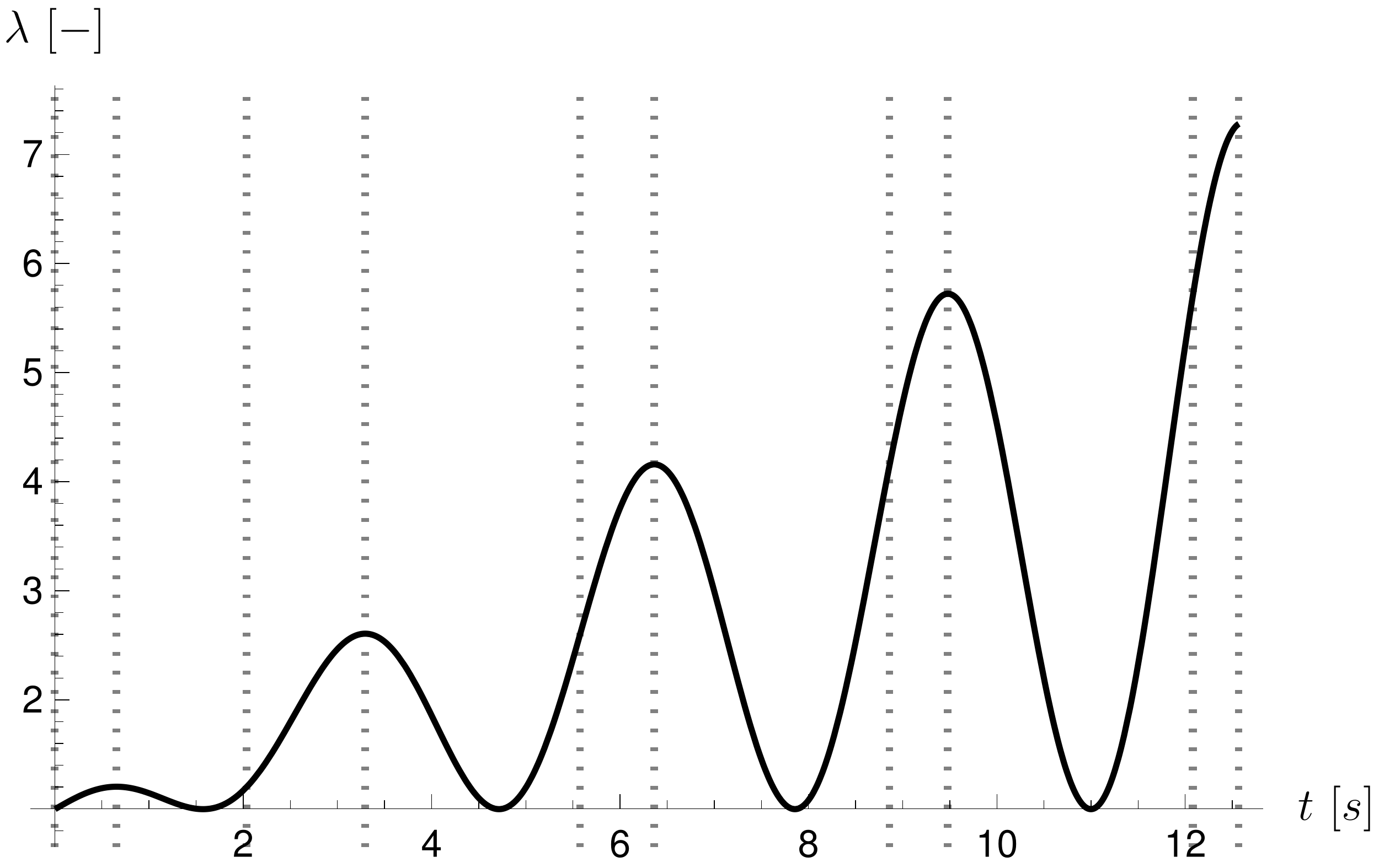
Refer to caption
Figure 2. Loading. Dotted vertical lines indicate time instants at which the material switches between the primary loading path and a secondary loading path.

4.1. Idealised Mullins effect

We assume that the Helmholtz free energy ψmech,A\psi^{\mathrm{mech},\mathrm{A}} for material of interest is the Helmholtz free energy for the incompressble neo-Hooke solid. Thus the mechanical part of the Helmholtz free energy is given by the formula

(4.5) ψmech,A=defμA2​ρR(Tr𝔹−3).\psi^{\mathrm{mech},\mathrm{A}}=_{\mathrm{def}}\frac{\mu^{\mathrm{A}}}{2\rho_{\mathrm{R}}}\left(\Tr\mathbb{B}-3\right).

which yields ∂ψmech,A∂𝔹=μA2​ρR​𝕀\frac{\partial{\psi^{\mathrm{mech},\mathrm{A}}}}{\partial{\mathbb{B}}}=\frac{\mu^{\mathrm{A}}}{2\rho_{\mathrm{R}}}\mathbb{I}. (Recall that for incompressible solid we have ρ=ρR\rho=\rho_{\mathrm{R}}.) Concerning the formula for φ\varphi, we stick to (3.24a). Formula (3.24c) for the Cauchy stress tensor in the incompressible case gives only the traceless (deviatoric) part of the Cauchy stress tensor,

(4.6) 𝕋δ=def2ρ(φ+ψmech,Aψmaxmech,Ad​φd​zA)(𝔹∂ψmech,A∂𝔹)δ.{\mathbb{T}}_{\delta}=_{\mathrm{def}}2\rho\left(\varphi+\frac{\psi^{\mathrm{mech},\mathrm{A}}}{\psi^{\mathrm{mech},\mathrm{A}}_{\mathrm{max}}}\frac{\mathrm{d}{\varphi}}{\mathrm{d}{z_{\mathrm{A}}}}\right){\left(\mathbb{B}\frac{\partial{\psi^{\mathrm{mech},\mathrm{A}}}}{\partial{\mathbb{B}}}\right)}_{\delta}.

For our choice of ψmech,A\psi^{\mathrm{mech},\mathrm{A}} this reduces to

(4.7) 𝕋δ=defμA(φ+ψmech,Aψmaxmech,Ad​φd​zA)𝔹δ,{\mathbb{T}}_{\delta}=_{\mathrm{def}}\mu^{\mathrm{A}}\left(\varphi+\frac{\psi^{\mathrm{mech},\mathrm{A}}}{\psi^{\mathrm{mech},\mathrm{A}}_{\mathrm{max}}}\frac{\mathrm{d}{\varphi}}{\mathrm{d}{z_{\mathrm{A}}}}\right){\mathbb{B}}_{\delta},

and for the uniaxial deformation we get

(4.8) [(Tδ)x^​x^000(Tδ)y^​y^000(Tδ)z^​z^]=μA​(φ+ψmech,Aψmaxmech,A​d​φd​zA)​[23​(λ2−1λ)000−13​(λ2−1λ)000−13​(λ2−1λ)],\begin{bmatrix}\mathchoice{{\left(\mathrm{T}_{\delta}\right)}^{{\mathchoice{\makebox[5.55557pt][c]{$\displaystyle$}}{\makebox[5.55557pt][c]{$\textstyle$}}{\makebox[5.55557pt][c]{$\scriptstyle$}}{\makebox[5.55557pt][c]{$\scriptscriptstyle$}}\mathchoice{\makebox[5.55557pt][c]{$\displaystyle$}}{\makebox[5.55557pt][c]{$\textstyle$}}{\makebox[5.55557pt][c]{$\scriptstyle$}}{\makebox[5.55557pt][c]{$\scriptscriptstyle$}}}}_{{{\hat{x}}{\hat{x}}}}}{{\left(\mathrm{T}_{\delta}\right)}^{{\mathchoice{\makebox[5.55557pt][c]{$\displaystyle$}}{\makebox[5.55557pt][c]{$\textstyle$}}{\makebox[5.55557pt][c]{$\scriptstyle$}}{\makebox[5.55557pt][c]{$\scriptscriptstyle$}}\mathchoice{\makebox[5.55557pt][c]{$\displaystyle$}}{\makebox[5.55557pt][c]{$\textstyle$}}{\makebox[5.55557pt][c]{$\scriptstyle$}}{\makebox[5.55557pt][c]{$\scriptscriptstyle$}}}}_{{{\hat{x}}{\hat{x}}}}}{{\left(\mathrm{T}_{\delta}\right)}^{{\mathchoice{\makebox[5.55557pt][c]{$\displaystyle$}}{\makebox[5.55557pt][c]{$\textstyle$}}{\makebox[5.55557pt][c]{$\scriptstyle$}}{\makebox[5.55557pt][c]{$\scriptscriptstyle$}}\mathchoice{\makebox[5.55557pt][c]{$\displaystyle$}}{\makebox[5.55557pt][c]{$\textstyle$}}{\makebox[5.55557pt][c]{$\scriptstyle$}}{\makebox[5.55557pt][c]{$\scriptscriptstyle$}}}}_{{{\hat{x}}{\hat{x}}}}}{{\left(\mathrm{T}_{\delta}\right)}^{{\mathchoice{\makebox[5.55557pt][c]{$\displaystyle$}}{\makebox[5.55557pt][c]{$\textstyle$}}{\makebox[5.55557pt][c]{$\scriptstyle$}}{\makebox[5.55557pt][c]{$\scriptscriptstyle$}}\mathchoice{\makebox[5.55557pt][c]{$\displaystyle$}}{\makebox[5.55557pt][c]{$\textstyle$}}{\makebox[5.55557pt][c]{$\scriptstyle$}}{\makebox[5.55557pt][c]{$\scriptscriptstyle$}}}}_{{{\hat{x}}{\hat{x}}}}}&0&0\\ 0&\mathchoice{{\left(\mathrm{T}_{\delta}\right)}^{{\mathchoice{\makebox[5.55557pt][c]{$\displaystyle$}}{\makebox[5.55557pt][c]{$\textstyle$}}{\makebox[5.55557pt][c]{$\scriptstyle$}}{\makebox[5.55557pt][c]{$\scriptscriptstyle$}}\mathchoice{\makebox[5.55557pt][c]{$\displaystyle$}}{\makebox[5.55557pt][c]{$\textstyle$}}{\makebox[5.55557pt][c]{$\scriptstyle$}}{\makebox[5.55557pt][c]{$\scriptscriptstyle$}}}}_{{{\hat{y}}{\hat{y}}}}}{{\left(\mathrm{T}_{\delta}\right)}^{{\mathchoice{\makebox[5.55557pt][c]{$\displaystyle$}}{\makebox[5.55557pt][c]{$\textstyle$}}{\makebox[5.55557pt][c]{$\scriptstyle$}}{\makebox[5.55557pt][c]{$\scriptscriptstyle$}}\mathchoice{\makebox[5.55557pt][c]{$\displaystyle$}}{\makebox[5.55557pt][c]{$\textstyle$}}{\makebox[5.55557pt][c]{$\scriptstyle$}}{\makebox[5.55557pt][c]{$\scriptscriptstyle$}}}}_{{{\hat{y}}{\hat{y}}}}}{{\left(\mathrm{T}_{\delta}\right)}^{{\mathchoice{\makebox[5.55557pt][c]{$\displaystyle$}}{\makebox[5.55557pt][c]{$\textstyle$}}{\makebox[5.55557pt][c]{$\scriptstyle$}}{\makebox[5.55557pt][c]{$\scriptscriptstyle$}}\mathchoice{\makebox[5.55557pt][c]{$\displaystyle$}}{\makebox[5.55557pt][c]{$\textstyle$}}{\makebox[5.55557pt][c]{$\scriptstyle$}}{\makebox[5.55557pt][c]{$\scriptscriptstyle$}}}}_{{{\hat{y}}{\hat{y}}}}}{{\left(\mathrm{T}_{\delta}\right)}^{{\mathchoice{\makebox[5.55557pt][c]{$\displaystyle$}}{\makebox[5.55557pt][c]{$\textstyle$}}{\makebox[5.55557pt][c]{$\scriptstyle$}}{\makebox[5.55557pt][c]{$\scriptscriptstyle$}}\mathchoice{\makebox[5.55557pt][c]{$\displaystyle$}}{\makebox[5.55557pt][c]{$\textstyle$}}{\makebox[5.55557pt][c]{$\scriptstyle$}}{\makebox[5.55557pt][c]{$\scriptscriptstyle$}}}}_{{{\hat{y}}{\hat{y}}}}}&0\\ 0&0&\mathchoice{{\left(\mathrm{T}_{\delta}\right)}^{{\mathchoice{\makebox[5.55557pt][c]{$\displaystyle$}}{\makebox[5.55557pt][c]{$\textstyle$}}{\makebox[5.55557pt][c]{$\scriptstyle$}}{\makebox[5.55557pt][c]{$\scriptscriptstyle$}}\mathchoice{\makebox[5.55557pt][c]{$\displaystyle$}}{\makebox[5.55557pt][c]{$\textstyle$}}{\makebox[5.55557pt][c]{$\scriptstyle$}}{\makebox[5.55557pt][c]{$\scriptscriptstyle$}}}}_{{{\hat{z}}{\hat{z}}}}}{{\left(\mathrm{T}_{\delta}\right)}^{{\mathchoice{\makebox[5.55557pt][c]{$\displaystyle$}}{\makebox[5.55557pt][c]{$\textstyle$}}{\makebox[5.55557pt][c]{$\scriptstyle$}}{\makebox[5.55557pt][c]{$\scriptscriptstyle$}}\mathchoice{\makebox[5.55557pt][c]{$\displaystyle$}}{\makebox[5.55557pt][c]{$\textstyle$}}{\makebox[5.55557pt][c]{$\scriptstyle$}}{\makebox[5.55557pt][c]{$\scriptscriptstyle$}}}}_{{{\hat{z}}{\hat{z}}}}}{{\left(\mathrm{T}_{\delta}\right)}^{{\mathchoice{\makebox[5.55557pt][c]{$\displaystyle$}}{\makebox[5.55557pt][c]{$\textstyle$}}{\makebox[5.55557pt][c]{$\scriptstyle$}}{\makebox[5.55557pt][c]{$\scriptscriptstyle$}}\mathchoice{\makebox[5.55557pt][c]{$\displaystyle$}}{\makebox[5.55557pt][c]{$\textstyle$}}{\makebox[5.55557pt][c]{$\scriptstyle$}}{\makebox[5.55557pt][c]{$\scriptscriptstyle$}}}}_{{{\hat{z}}{\hat{z}}}}}{{\left(\mathrm{T}_{\delta}\right)}^{{\mathchoice{\makebox[5.55557pt][c]{$\displaystyle$}}{\makebox[5.55557pt][c]{$\textstyle$}}{\makebox[5.55557pt][c]{$\scriptstyle$}}{\makebox[5.55557pt][c]{$\scriptscriptstyle$}}\mathchoice{\makebox[5.55557pt][c]{$\displaystyle$}}{\makebox[5.55557pt][c]{$\textstyle$}}{\makebox[5.55557pt][c]{$\scriptstyle$}}{\makebox[5.55557pt][c]{$\scriptscriptstyle$}}}}_{{{\hat{z}}{\hat{z}}}}}\end{bmatrix}=\mu^{\mathrm{A}}\left(\varphi+\frac{\psi^{\mathrm{mech},\mathrm{A}}}{\psi^{\mathrm{mech},\mathrm{A}}_{\mathrm{max}}}\frac{\mathrm{d}{\varphi}}{\mathrm{d}{z_{\mathrm{A}}}}\right)\begin{bmatrix}\frac{2}{3}\left(\lambda^{2}-\frac{1}{\lambda}\right)&0&0\\ 0&-\frac{1}{3}\left(\lambda^{2}-\frac{1}{\lambda}\right)&0\\ 0&0&-\frac{1}{3}\left(\lambda^{2}-\frac{1}{\lambda}\right)\end{bmatrix},

where (Tδ)y^​y^=(Tδ)z^​z^\mathchoice{{\left(\mathrm{T}_{\delta}\right)}^{{\mathchoice{\makebox[5.55557pt][c]{$\displaystyle$}}{\makebox[5.55557pt][c]{$\textstyle$}}{\makebox[5.55557pt][c]{$\scriptstyle$}}{\makebox[5.55557pt][c]{$\scriptscriptstyle$}}\mathchoice{\makebox[5.55557pt][c]{$\displaystyle$}}{\makebox[5.55557pt][c]{$\textstyle$}}{\makebox[5.55557pt][c]{$\scriptstyle$}}{\makebox[5.55557pt][c]{$\scriptscriptstyle$}}}}_{{{\hat{y}}{\hat{y}}}}}{{\left(\mathrm{T}_{\delta}\right)}^{{\mathchoice{\makebox[5.55557pt][c]{$\displaystyle$}}{\makebox[5.55557pt][c]{$\textstyle$}}{\makebox[5.55557pt][c]{$\scriptstyle$}}{\makebox[5.55557pt][c]{$\scriptscriptstyle$}}\mathchoice{\makebox[5.55557pt][c]{$\displaystyle$}}{\makebox[5.55557pt][c]{$\textstyle$}}{\makebox[5.55557pt][c]{$\scriptstyle$}}{\makebox[5.55557pt][c]{$\scriptscriptstyle$}}}}_{{{\hat{y}}{\hat{y}}}}}{{\left(\mathrm{T}_{\delta}\right)}^{{\mathchoice{\makebox[5.55557pt][c]{$\displaystyle$}}{\makebox[5.55557pt][c]{$\textstyle$}}{\makebox[5.55557pt][c]{$\scriptstyle$}}{\makebox[5.55557pt][c]{$\scriptscriptstyle$}}\mathchoice{\makebox[5.55557pt][c]{$\displaystyle$}}{\makebox[5.55557pt][c]{$\textstyle$}}{\makebox[5.55557pt][c]{$\scriptstyle$}}{\makebox[5.55557pt][c]{$\scriptscriptstyle$}}}}_{{{\hat{y}}{\hat{y}}}}}{{\left(\mathrm{T}_{\delta}\right)}^{{\mathchoice{\makebox[5.55557pt][c]{$\displaystyle$}}{\makebox[5.55557pt][c]{$\textstyle$}}{\makebox[5.55557pt][c]{$\scriptstyle$}}{\makebox[5.55557pt][c]{$\scriptscriptstyle$}}\mathchoice{\makebox[5.55557pt][c]{$\displaystyle$}}{\makebox[5.55557pt][c]{$\textstyle$}}{\makebox[5.55557pt][c]{$\scriptstyle$}}{\makebox[5.55557pt][c]{$\scriptscriptstyle$}}}}_{{{\hat{y}}{\hat{y}}}}}=\mathchoice{{\left(\mathrm{T}_{\delta}\right)}^{{\mathchoice{\makebox[5.55557pt][c]{$\displaystyle$}}{\makebox[5.55557pt][c]{$\textstyle$}}{\makebox[5.55557pt][c]{$\scriptstyle$}}{\makebox[5.55557pt][c]{$\scriptscriptstyle$}}\mathchoice{\makebox[5.55557pt][c]{$\displaystyle$}}{\makebox[5.55557pt][c]{$\textstyle$}}{\makebox[5.55557pt][c]{$\scriptstyle$}}{\makebox[5.55557pt][c]{$\scriptscriptstyle$}}}}_{{{\hat{z}}{\hat{z}}}}}{{\left(\mathrm{T}_{\delta}\right)}^{{\mathchoice{\makebox[5.55557pt][c]{$\displaystyle$}}{\makebox[5.55557pt][c]{$\textstyle$}}{\makebox[5.55557pt][c]{$\scriptstyle$}}{\makebox[5.55557pt][c]{$\scriptscriptstyle$}}\mathchoice{\makebox[5.55557pt][c]{$\displaystyle$}}{\makebox[5.55557pt][c]{$\textstyle$}}{\makebox[5.55557pt][c]{$\scriptstyle$}}{\makebox[5.55557pt][c]{$\scriptscriptstyle$}}}}_{{{\hat{z}}{\hat{z}}}}}{{\left(\mathrm{T}_{\delta}\right)}^{{\mathchoice{\makebox[5.55557pt][c]{$\displaystyle$}}{\makebox[5.55557pt][c]{$\textstyle$}}{\makebox[5.55557pt][c]{$\scriptstyle$}}{\makebox[5.55557pt][c]{$\scriptscriptstyle$}}\mathchoice{\makebox[5.55557pt][c]{$\displaystyle$}}{\makebox[5.55557pt][c]{$\textstyle$}}{\makebox[5.55557pt][c]{$\scriptstyle$}}{\makebox[5.55557pt][c]{$\scriptscriptstyle$}}}}_{{{\hat{z}}{\hat{z}}}}}{{\left(\mathrm{T}_{\delta}\right)}^{{\mathchoice{\makebox[5.55557pt][c]{$\displaystyle$}}{\makebox[5.55557pt][c]{$\textstyle$}}{\makebox[5.55557pt][c]{$\scriptstyle$}}{\makebox[5.55557pt][c]{$\scriptscriptstyle$}}\mathchoice{\makebox[5.55557pt][c]{$\displaystyle$}}{\makebox[5.55557pt][c]{$\textstyle$}}{\makebox[5.55557pt][c]{$\scriptstyle$}}{\makebox[5.55557pt][c]{$\scriptscriptstyle$}}}}_{{{\hat{z}}{\hat{z}}}}} and (Tδ)y^​y^=−12​(Tδ)x^​x^\mathchoice{{\left(\mathrm{T}_{\delta}\right)}^{{\mathchoice{\makebox[5.55557pt][c]{$\displaystyle$}}{\makebox[5.55557pt][c]{$\textstyle$}}{\makebox[5.55557pt][c]{$\scriptstyle$}}{\makebox[5.55557pt][c]{$\scriptscriptstyle$}}\mathchoice{\makebox[5.55557pt][c]{$\displaystyle$}}{\makebox[5.55557pt][c]{$\textstyle$}}{\makebox[5.55557pt][c]{$\scriptstyle$}}{\makebox[5.55557pt][c]{$\scriptscriptstyle$}}}}_{{{\hat{y}}{\hat{y}}}}}{{\left(\mathrm{T}_{\delta}\right)}^{{\mathchoice{\makebox[5.55557pt][c]{$\displaystyle$}}{\makebox[5.55557pt][c]{$\textstyle$}}{\makebox[5.55557pt][c]{$\scriptstyle$}}{\makebox[5.55557pt][c]{$\scriptscriptstyle$}}\mathchoice{\makebox[5.55557pt][c]{$\displaystyle$}}{\makebox[5.55557pt][c]{$\textstyle$}}{\makebox[5.55557pt][c]{$\scriptstyle$}}{\makebox[5.55557pt][c]{$\scriptscriptstyle$}}}}_{{{\hat{y}}{\hat{y}}}}}{{\left(\mathrm{T}_{\delta}\right)}^{{\mathchoice{\makebox[5.55557pt][c]{$\displaystyle$}}{\makebox[5.55557pt][c]{$\textstyle$}}{\makebox[5.55557pt][c]{$\scriptstyle$}}{\makebox[5.55557pt][c]{$\scriptscriptstyle$}}\mathchoice{\makebox[5.55557pt][c]{$\displaystyle$}}{\makebox[5.55557pt][c]{$\textstyle$}}{\makebox[5.55557pt][c]{$\scriptstyle$}}{\makebox[5.55557pt][c]{$\scriptscriptstyle$}}}}_{{{\hat{y}}{\hat{y}}}}}{{\left(\mathrm{T}_{\delta}\right)}^{{\mathchoice{\makebox[5.55557pt][c]{$\displaystyle$}}{\makebox[5.55557pt][c]{$\textstyle$}}{\makebox[5.55557pt][c]{$\scriptstyle$}}{\makebox[5.55557pt][c]{$\scriptscriptstyle$}}\mathchoice{\makebox[5.55557pt][c]{$\displaystyle$}}{\makebox[5.55557pt][c]{$\textstyle$}}{\makebox[5.55557pt][c]{$\scriptstyle$}}{\makebox[5.55557pt][c]{$\scriptscriptstyle$}}}}_{{{\hat{y}}{\hat{y}}}}}=-\frac{1}{2}\mathchoice{{\left(\mathrm{T}_{\delta}\right)}^{{\mathchoice{\makebox[5.55557pt][c]{$\displaystyle$}}{\makebox[5.55557pt][c]{$\textstyle$}}{\makebox[5.55557pt][c]{$\scriptstyle$}}{\makebox[5.55557pt][c]{$\scriptscriptstyle$}}\mathchoice{\makebox[5.55557pt][c]{$\displaystyle$}}{\makebox[5.55557pt][c]{$\textstyle$}}{\makebox[5.55557pt][c]{$\scriptstyle$}}{\makebox[5.55557pt][c]{$\scriptscriptstyle$}}}}_{{{\hat{x}}{\hat{x}}}}}{{\left(\mathrm{T}_{\delta}\right)}^{{\mathchoice{\makebox[5.55557pt][c]{$\displaystyle$}}{\makebox[5.55557pt][c]{$\textstyle$}}{\makebox[5.55557pt][c]{$\scriptstyle$}}{\makebox[5.55557pt][c]{$\scriptscriptstyle$}}\mathchoice{\makebox[5.55557pt][c]{$\displaystyle$}}{\makebox[5.55557pt][c]{$\textstyle$}}{\makebox[5.55557pt][c]{$\scriptstyle$}}{\makebox[5.55557pt][c]{$\scriptscriptstyle$}}}}_{{{\hat{x}}{\hat{x}}}}}{{\left(\mathrm{T}_{\delta}\right)}^{{\mathchoice{\makebox[5.55557pt][c]{$\displaystyle$}}{\makebox[5.55557pt][c]{$\textstyle$}}{\makebox[5.55557pt][c]{$\scriptstyle$}}{\makebox[5.55557pt][c]{$\scriptscriptstyle$}}\mathchoice{\makebox[5.55557pt][c]{$\displaystyle$}}{\makebox[5.55557pt][c]{$\textstyle$}}{\makebox[5.55557pt][c]{$\scriptstyle$}}{\makebox[5.55557pt][c]{$\scriptscriptstyle$}}}}_{{{\hat{x}}{\hat{x}}}}}{{\left(\mathrm{T}_{\delta}\right)}^{{\mathchoice{\makebox[5.55557pt][c]{$\displaystyle$}}{\makebox[5.55557pt][c]{$\textstyle$}}{\makebox[5.55557pt][c]{$\scriptstyle$}}{\makebox[5.55557pt][c]{$\scriptscriptstyle$}}\mathchoice{\makebox[5.55557pt][c]{$\displaystyle$}}{\makebox[5.55557pt][c]{$\textstyle$}}{\makebox[5.55557pt][c]{$\scriptstyle$}}{\makebox[5.55557pt][c]{$\scriptscriptstyle$}}}}_{{{\hat{x}}{\hat{x}}}}}. We also see that in our particular case we have

(4.9) ψmech,A=μA2​ρR​[(λ2+2λ)−3].\psi^{\mathrm{mech},\mathrm{A}}=\frac{\mu^{\mathrm{A}}}{2\rho_{\mathrm{R}}}\left[\left(\lambda^{2}+\frac{2}{\lambda}\right)-3\right].

Consequently, the problem we need to solve is the following. For given λ\lambda, see (4.2), find (Tδ)x^​x^\mathchoice{{\left(\mathrm{T}_{\delta}\right)}^{{\mathchoice{\makebox[5.55557pt][c]{$\displaystyle$}}{\makebox[5.55557pt][c]{$\textstyle$}}{\makebox[5.55557pt][c]{$\scriptstyle$}}{\makebox[5.55557pt][c]{$\scriptscriptstyle$}}\mathchoice{\makebox[5.55557pt][c]{$\displaystyle$}}{\makebox[5.55557pt][c]{$\textstyle$}}{\makebox[5.55557pt][c]{$\scriptstyle$}}{\makebox[5.55557pt][c]{$\scriptscriptstyle$}}}}_{{{\hat{x}}{\hat{x}}}}}{{\left(\mathrm{T}_{\delta}\right)}^{{\mathchoice{\makebox[5.55557pt][c]{$\displaystyle$}}{\makebox[5.55557pt][c]{$\textstyle$}}{\makebox[5.55557pt][c]{$\scriptstyle$}}{\makebox[5.55557pt][c]{$\scriptscriptstyle$}}\mathchoice{\makebox[5.55557pt][c]{$\displaystyle$}}{\makebox[5.55557pt][c]{$\textstyle$}}{\makebox[5.55557pt][c]{$\scriptstyle$}}{\makebox[5.55557pt][c]{$\scriptscriptstyle$}}}}_{{{\hat{x}}{\hat{x}}}}}{{\left(\mathrm{T}_{\delta}\right)}^{{\mathchoice{\makebox[5.55557pt][c]{$\displaystyle$}}{\makebox[5.55557pt][c]{$\textstyle$}}{\makebox[5.55557pt][c]{$\scriptstyle$}}{\makebox[5.55557pt][c]{$\scriptscriptstyle$}}\mathchoice{\makebox[5.55557pt][c]{$\displaystyle$}}{\makebox[5.55557pt][c]{$\textstyle$}}{\makebox[5.55557pt][c]{$\scriptstyle$}}{\makebox[5.55557pt][c]{$\scriptscriptstyle$}}}}_{{{\hat{x}}{\hat{x}}}}}{{\left(\mathrm{T}_{\delta}\right)}^{{\mathchoice{\makebox[5.55557pt][c]{$\displaystyle$}}{\makebox[5.55557pt][c]{$\textstyle$}}{\makebox[5.55557pt][c]{$\scriptstyle$}}{\makebox[5.55557pt][c]{$\scriptscriptstyle$}}\mathchoice{\makebox[5.55557pt][c]{$\displaystyle$}}{\makebox[5.55557pt][c]{$\textstyle$}}{\makebox[5.55557pt][c]{$\scriptstyle$}}{\makebox[5.55557pt][c]{$\scriptscriptstyle$}}}}_{{{\hat{x}}{\hat{x}}}}} such that

(4.10a) (Tδ)x^​x^\displaystyle\mathchoice{{\left(\mathrm{T}_{\delta}\right)}^{{\mathchoice{\makebox[5.55557pt][c]{$\displaystyle$}}{\makebox[5.55557pt][c]{$\textstyle$}}{\makebox[5.55557pt][c]{$\scriptstyle$}}{\makebox[5.55557pt][c]{$\scriptscriptstyle$}}\mathchoice{\makebox[5.55557pt][c]{$\displaystyle$}}{\makebox[5.55557pt][c]{$\textstyle$}}{\makebox[5.55557pt][c]{$\scriptstyle$}}{\makebox[5.55557pt][c]{$\scriptscriptstyle$}}}}_{{{\hat{x}}{\hat{x}}}}}{{\left(\mathrm{T}_{\delta}\right)}^{{\mathchoice{\makebox[5.55557pt][c]{$\displaystyle$}}{\makebox[5.55557pt][c]{$\textstyle$}}{\makebox[5.55557pt][c]{$\scriptstyle$}}{\makebox[5.55557pt][c]{$\scriptscriptstyle$}}\mathchoice{\makebox[5.55557pt][c]{$\displaystyle$}}{\makebox[5.55557pt][c]{$\textstyle$}}{\makebox[5.55557pt][c]{$\scriptstyle$}}{\makebox[5.55557pt][c]{$\scriptscriptstyle$}}}}_{{{\hat{x}}{\hat{x}}}}}{{\left(\mathrm{T}_{\delta}\right)}^{{\mathchoice{\makebox[5.55557pt][c]{$\displaystyle$}}{\makebox[5.55557pt][c]{$\textstyle$}}{\makebox[5.55557pt][c]{$\scriptstyle$}}{\makebox[5.55557pt][c]{$\scriptscriptstyle$}}\mathchoice{\makebox[5.55557pt][c]{$\displaystyle$}}{\makebox[5.55557pt][c]{$\textstyle$}}{\makebox[5.55557pt][c]{$\scriptstyle$}}{\makebox[5.55557pt][c]{$\scriptscriptstyle$}}}}_{{{\hat{x}}{\hat{x}}}}}{{\left(\mathrm{T}_{\delta}\right)}^{{\mathchoice{\makebox[5.55557pt][c]{$\displaystyle$}}{\makebox[5.55557pt][c]{$\textstyle$}}{\makebox[5.55557pt][c]{$\scriptstyle$}}{\makebox[5.55557pt][c]{$\scriptscriptstyle$}}\mathchoice{\makebox[5.55557pt][c]{$\displaystyle$}}{\makebox[5.55557pt][c]{$\textstyle$}}{\makebox[5.55557pt][c]{$\scriptstyle$}}{\makebox[5.55557pt][c]{$\scriptscriptstyle$}}}}_{{{\hat{x}}{\hat{x}}}}} =μA​(φ+ψmech,Aψmaxmech,A​d​φd​zA)​23​(λ2−1λ),\displaystyle=\mu^{\mathrm{A}}\left(\varphi+\frac{\psi^{\mathrm{mech},\mathrm{A}}}{\psi^{\mathrm{mech},\mathrm{A}}_{\mathrm{max}}}\frac{\mathrm{d}{\varphi}}{\mathrm{d}{z_{\mathrm{A}}}}\right)\frac{2}{3}\left(\lambda^{2}-\frac{1}{\lambda}\right),
(4.10b) φ\displaystyle\varphi =∫ζ=0zAc⁡(ζ)​𝑑ζ+12zA+1,\displaystyle=\frac{\int_{\zeta=0}^{z_{\mathrm{A}}}c(\zeta)\,\mathrm{d}\zeta+\frac{1}{2}}{z_{\mathrm{A}}+1},
(4.10c) c\displaystyle c =(1−cmin)​(zA+1)​ea​zA+cmin,\displaystyle=\left(1-c_{\mathrm{min}}\right)\left(z_{\mathrm{A}}+1\right){\mathrm{e}}^{az_{\mathrm{A}}}+c_{\mathrm{min}},
(4.10d) zA\displaystyle z_{\mathrm{A}} ={ψmech,A−ψmaxmech,Aψmaxmech,A,ψmaxmech,A>0,0,ψmaxmech,A=0,\displaystyle=\begin{cases}\frac{\psi^{\mathrm{mech},\mathrm{A}}-\psi^{\mathrm{mech},\mathrm{A}}_{\mathrm{max}}}{\psi^{\mathrm{mech},\mathrm{A}}_{\mathrm{max}}},&\psi^{\mathrm{mech},\mathrm{A}}_{\mathrm{max}}>0,\\ 0,&\psi^{\mathrm{mech},\mathrm{A}}_{\mathrm{max}}=0,\\ \end{cases}
(4.10e) ψmech,A\displaystyle\psi^{\mathrm{mech},\mathrm{A}} =μA2​ρR​[(λ2+2λ)−3],\displaystyle=\frac{\mu^{\mathrm{A}}}{2\rho_{\mathrm{R}}}\left[\left(\lambda^{2}+\frac{2}{\lambda}\right)-3\right],
(4.10f) d​ψmaxmech,Ad​t\displaystyle\frac{\mathrm{d}{\psi^{\mathrm{mech},\mathrm{A}}_{\mathrm{max}}}}{\mathrm{d}{t}} =H⁡(zA)​H​(𝕋​\vdotdot​𝔻)​|d​ψmech,Ad​t|,\displaystyle=H\left(z_{\mathrm{A}}\right)H\left(\mathbb{T}\vdotdot\mathbb{D}\right)\left|\frac{\mathrm{d}{\psi^{\mathrm{mech},\mathrm{A}}}}{\mathrm{d}{t}}\right|,

while the initial condition for ψmaxmech,A\psi^{\mathrm{mech},\mathrm{A}}_{\mathrm{max}} is ψmaxmech,A|t=0=0\left.\psi^{\mathrm{mech},\mathrm{A}}_{\mathrm{max}}\right|_{t=0}=0. This system of equations is straightforward to solve numerically—it consists of one ordinary differential equation (4.10f) and one algebraic equation (4.10a). Equations (4.10b), (4.10d) and (4.10e) are just definitions for the corresponding symbols.

We note that in order to ease the numerical solution of (4.10), the argument of the Heaviside function in (4.10f) can be further simplified. In virtue of (4.10a) we see that

(4.11) 𝕋​\vdotdot​𝔻=23​μA​(φ+ψmech,Aψmaxmech,A​d​φd​zA)​(λ2−1λ)​1λ​d​λd​t,\mathbb{T}\vdotdot\mathbb{D}=\frac{2}{3}\mu^{\mathrm{A}}\left(\varphi+\frac{\psi^{\mathrm{mech},\mathrm{A}}}{\psi^{\mathrm{mech},\mathrm{A}}_{\mathrm{max}}}\frac{\mathrm{d}{\varphi}}{\mathrm{d}{z_{\mathrm{A}}}}\right)\left(\lambda^{2}-\frac{1}{\lambda}\right)\frac{1}{\lambda}\frac{\mathrm{d}{\lambda}}{\mathrm{d}{t}},

hence we can simplify H⁡(𝕋​\vdotdot​𝔻)H\left(\mathbb{T}\vdotdot\mathbb{D}\right) as

(4.12) H⁡(𝕋​\vdotdot​𝔻)=H⁡((λ−1)​d​λd​t).H\left(\mathbb{T}\vdotdot\mathbb{D}\right)=H\left(\left(\lambda-1\right)\frac{\mathrm{d}{\lambda}}{\mathrm{d}{t}}\right).

We have solved (4.10) numerically for artificial material parameter values μA\mu^{\mathrm{A}} and ρ\rho, and the corresponding stretch–stress diagram is shown in Figure 3. Clearly, the material responds as expected—we see the idealised version of the Mullins effect. The analysis in Section 3.2, see the discussion following equation (3.11), reveals that the stress must be bounded from below and above. The top envelope is given by

(4.13) (Ttop,δ)x^​x^=μA​23​(λ2−1λ),\mathchoice{{\left(\mathrm{T}_{\mathrm{top},\delta}\right)}^{{\mathchoice{\makebox[5.55557pt][c]{$\displaystyle$}}{\makebox[5.55557pt][c]{$\textstyle$}}{\makebox[5.55557pt][c]{$\scriptstyle$}}{\makebox[5.55557pt][c]{$\scriptscriptstyle$}}\mathchoice{\makebox[5.55557pt][c]{$\displaystyle$}}{\makebox[5.55557pt][c]{$\textstyle$}}{\makebox[5.55557pt][c]{$\scriptstyle$}}{\makebox[5.55557pt][c]{$\scriptscriptstyle$}}}}_{{{\hat{x}}{\hat{x}}}}}{{\left(\mathrm{T}_{\mathrm{top},\delta}\right)}^{{\mathchoice{\makebox[5.55557pt][c]{$\displaystyle$}}{\makebox[5.55557pt][c]{$\textstyle$}}{\makebox[5.55557pt][c]{$\scriptstyle$}}{\makebox[5.55557pt][c]{$\scriptscriptstyle$}}\mathchoice{\makebox[5.55557pt][c]{$\displaystyle$}}{\makebox[5.55557pt][c]{$\textstyle$}}{\makebox[5.55557pt][c]{$\scriptstyle$}}{\makebox[5.55557pt][c]{$\scriptscriptstyle$}}}}_{{{\hat{x}}{\hat{x}}}}}{{\left(\mathrm{T}_{\mathrm{top},\delta}\right)}^{{\mathchoice{\makebox[5.55557pt][c]{$\displaystyle$}}{\makebox[5.55557pt][c]{$\textstyle$}}{\makebox[5.55557pt][c]{$\scriptstyle$}}{\makebox[5.55557pt][c]{$\scriptscriptstyle$}}\mathchoice{\makebox[5.55557pt][c]{$\displaystyle$}}{\makebox[5.55557pt][c]{$\textstyle$}}{\makebox[5.55557pt][c]{$\scriptstyle$}}{\makebox[5.55557pt][c]{$\scriptscriptstyle$}}}}_{{{\hat{x}}{\hat{x}}}}}{{\left(\mathrm{T}_{\mathrm{top},\delta}\right)}^{{\mathchoice{\makebox[5.55557pt][c]{$\displaystyle$}}{\makebox[5.55557pt][c]{$\textstyle$}}{\makebox[5.55557pt][c]{$\scriptstyle$}}{\makebox[5.55557pt][c]{$\scriptscriptstyle$}}\mathchoice{\makebox[5.55557pt][c]{$\displaystyle$}}{\makebox[5.55557pt][c]{$\textstyle$}}{\makebox[5.55557pt][c]{$\scriptstyle$}}{\makebox[5.55557pt][c]{$\scriptscriptstyle$}}}}_{{{\hat{x}}{\hat{x}}}}}=\mu^{\mathrm{A}}\frac{2}{3}\left(\lambda^{2}-\frac{1}{\lambda}\right),

while the bottom envelope is given by

(4.14) (Tbot,δ)x^​x^=μA2​23​(λ2−1λ).\mathchoice{{\left(\mathrm{T}_{\mathrm{bot},\delta}\right)}^{{\mathchoice{\makebox[5.55557pt][c]{$\displaystyle$}}{\makebox[5.55557pt][c]{$\textstyle$}}{\makebox[5.55557pt][c]{$\scriptstyle$}}{\makebox[5.55557pt][c]{$\scriptscriptstyle$}}\mathchoice{\makebox[5.55557pt][c]{$\displaystyle$}}{\makebox[5.55557pt][c]{$\textstyle$}}{\makebox[5.55557pt][c]{$\scriptstyle$}}{\makebox[5.55557pt][c]{$\scriptscriptstyle$}}}}_{{{\hat{x}}{\hat{x}}}}}{{\left(\mathrm{T}_{\mathrm{bot},\delta}\right)}^{{\mathchoice{\makebox[5.55557pt][c]{$\displaystyle$}}{\makebox[5.55557pt][c]{$\textstyle$}}{\makebox[5.55557pt][c]{$\scriptstyle$}}{\makebox[5.55557pt][c]{$\scriptscriptstyle$}}\mathchoice{\makebox[5.55557pt][c]{$\displaystyle$}}{\makebox[5.55557pt][c]{$\textstyle$}}{\makebox[5.55557pt][c]{$\scriptstyle$}}{\makebox[5.55557pt][c]{$\scriptscriptstyle$}}}}_{{{\hat{x}}{\hat{x}}}}}{{\left(\mathrm{T}_{\mathrm{bot},\delta}\right)}^{{\mathchoice{\makebox[5.55557pt][c]{$\displaystyle$}}{\makebox[5.55557pt][c]{$\textstyle$}}{\makebox[5.55557pt][c]{$\scriptstyle$}}{\makebox[5.55557pt][c]{$\scriptscriptstyle$}}\mathchoice{\makebox[5.55557pt][c]{$\displaystyle$}}{\makebox[5.55557pt][c]{$\textstyle$}}{\makebox[5.55557pt][c]{$\scriptstyle$}}{\makebox[5.55557pt][c]{$\scriptscriptstyle$}}}}_{{{\hat{x}}{\hat{x}}}}}{{\left(\mathrm{T}_{\mathrm{bot},\delta}\right)}^{{\mathchoice{\makebox[5.55557pt][c]{$\displaystyle$}}{\makebox[5.55557pt][c]{$\textstyle$}}{\makebox[5.55557pt][c]{$\scriptstyle$}}{\makebox[5.55557pt][c]{$\scriptscriptstyle$}}\mathchoice{\makebox[5.55557pt][c]{$\displaystyle$}}{\makebox[5.55557pt][c]{$\textstyle$}}{\makebox[5.55557pt][c]{$\scriptstyle$}}{\makebox[5.55557pt][c]{$\scriptscriptstyle$}}}}_{{{\hat{x}}{\hat{x}}}}}=\frac{\mu^{\mathrm{A}}}{2}\frac{2}{3}\left(\lambda^{2}-\frac{1}{\lambda}\right).

We show this envelopes in Figure 3 as well, and we see that the bounds work as predicted by the theory. Figure 3 also documents the role of parameter aa in the formula for function φ\varphi, see (4.10b). The higher the parameter value, the faster the secondary loading curve approaches the bottom envelope. This observation documents the flexibility of the model with respect to fitting potential experimental data.

Refer to caption
(a) a=0.01a=0.01
Refer to caption
(b) a=1a=1
Refer to caption
(c) a=10a=10
Figure 3. Idealised Mullins effect, Cauchy stress tensor component (Tδ)x^​x^\mathchoice{{\left(\mathrm{T}_{\delta}\right)}^{{\mathchoice{\makebox[5.55557pt][c]{$\displaystyle$}}{\makebox[5.55557pt][c]{$\textstyle$}}{\makebox[5.55557pt][c]{$\scriptstyle$}}{\makebox[5.55557pt][c]{$\scriptscriptstyle$}}\mathchoice{\makebox[5.55557pt][c]{$\displaystyle$}}{\makebox[5.55557pt][c]{$\textstyle$}}{\makebox[5.55557pt][c]{$\scriptstyle$}}{\makebox[5.55557pt][c]{$\scriptscriptstyle$}}}}_{{{\hat{x}}{\hat{x}}}}}{{\left(\mathrm{T}_{\delta}\right)}^{{\mathchoice{\makebox[5.55557pt][c]{$\displaystyle$}}{\makebox[5.55557pt][c]{$\textstyle$}}{\makebox[5.55557pt][c]{$\scriptstyle$}}{\makebox[5.55557pt][c]{$\scriptscriptstyle$}}\mathchoice{\makebox[5.55557pt][c]{$\displaystyle$}}{\makebox[5.55557pt][c]{$\textstyle$}}{\makebox[5.55557pt][c]{$\scriptstyle$}}{\makebox[5.55557pt][c]{$\scriptscriptstyle$}}}}_{{{\hat{x}}{\hat{x}}}}}{{\left(\mathrm{T}_{\delta}\right)}^{{\mathchoice{\makebox[5.55557pt][c]{$\displaystyle$}}{\makebox[5.55557pt][c]{$\textstyle$}}{\makebox[5.55557pt][c]{$\scriptstyle$}}{\makebox[5.55557pt][c]{$\scriptscriptstyle$}}\mathchoice{\makebox[5.55557pt][c]{$\displaystyle$}}{\makebox[5.55557pt][c]{$\textstyle$}}{\makebox[5.55557pt][c]{$\scriptstyle$}}{\makebox[5.55557pt][c]{$\scriptscriptstyle$}}}}_{{{\hat{x}}{\hat{x}}}}}{{\left(\mathrm{T}_{\delta}\right)}^{{\mathchoice{\makebox[5.55557pt][c]{$\displaystyle$}}{\makebox[5.55557pt][c]{$\textstyle$}}{\makebox[5.55557pt][c]{$\scriptstyle$}}{\makebox[5.55557pt][c]{$\scriptscriptstyle$}}\mathchoice{\makebox[5.55557pt][c]{$\displaystyle$}}{\makebox[5.55557pt][c]{$\textstyle$}}{\makebox[5.55557pt][c]{$\scriptstyle$}}{\makebox[5.55557pt][c]{$\scriptscriptstyle$}}}}_{{{\hat{x}}{\hat{x}}}}} versus stretch λ\lambda. Various choices of parameter aa in the formula for function φ\varphi, see (4.10b) and (4.10c); cmin=12c_{\mathrm{min}}=\frac{1}{2}, μA=1​MPa\mu^{\mathrm{A}}=1\,\mathrm{MPa}, ρ=1100​kg/m3\rho=1100\,\nicefrac{\mathrm{kg}}{\mathrm{m^{3}}}.

In Figure 4 we show the evolution of ψmaxmech,A\psi^{\mathrm{mech},\mathrm{A}}_{\mathrm{max}}, that is the solution to (4.10f). As expected, ψmaxmech,A\psi^{\mathrm{mech},\mathrm{A}}_{\mathrm{max}} is a non-decreasing function of time. Furthermore, the dotted vertical lines indicate the time instants at which the material switches between the primary loading path and secondary loading/unloading paths. The same time instants are also plotted in Figure 2. As expected, the growth/constancy of ψmaxmech,A\psi^{\mathrm{mech},\mathrm{A}}_{\mathrm{max}} corresponds in our simple setting to the growth/constancy of λmax\lambda_{\max}, where λmax\lambda_{\max} denotes the maximum stretch reached thorough the whole deformation history.

Refer to caption
(a) Initial time interval.
Refer to caption
(b) Complete time interval.
Figure 4. Helmholtz free energy ψmech,A\psi^{\mathrm{mech},\mathrm{A}} and ψmaxmech,A\psi^{\mathrm{mech},\mathrm{A}}_{\mathrm{max}}. Dotted vertical lines indicate time instants at which the material switches between the primary loading path and a secondary loading path.

4.2. Mullins effect with permanent strain

Concerning the model for permanent strain (3.53), we fix c⁡(zA)c(z_{\mathrm{A}}) and consequently φ⁡(zA)\varphi(z_{\mathrm{A}}) as in the previous section, see (4.10b) and (4.10c), with parameter values a=1a=1 and cmin=12c_{\mathrm{min}}=\frac{1}{2}. The Helmholtz free energy ψmech,A\psi^{\mathrm{mech},\mathrm{A}} is chosen as in the previous section, while the Helmholtz free energy ψmech,B\psi^{\mathrm{mech},\mathrm{B}} is chosen in the standard neo-Hooke form as well, that is

(4.15) ψmech,B=defμB2​ρR(Tr𝔹NC−3).\psi^{\mathrm{mech},\mathrm{B}}=_{\mathrm{def}}\frac{\mu^{\mathrm{B}}}{2\rho_{\mathrm{R}}}\left(\Tr\mathbb{B}_{\mathrm{NC}}-3\right).

Concerning the reference value ψrefmech,B\psi^{\mathrm{mech},\mathrm{B}}_{\mathrm{ref}} we set ψmech,Bref=defμB2​ρR\psi^{\mathrm{mech},\mathrm{B}}_{\mathrm{ref}}=_{\mathrm{def}}\frac{\mu^{\mathrm{B}}}{2\rho_{\mathrm{R}}}. For μB\mu^{\mathrm{B}} we set μB=def23μA\mu^{\mathrm{B}}=_{\mathrm{def}}\frac{2}{3}\mu^{\mathrm{A}}.

Equations for quantities φ\varphi, 𝕋A\mathbb{T}_{\mathrm{A}} and ψmaxmech\psi^{\mathrm{mech}}_{\mathrm{max}}, that is equations (3.24a), (3.24c) and (3.24d), are in the present case the same as in the previously studied case of the idealised Mullins effect. The only difference is that the formula for the stress (4.6) now gives us only 𝕋A\mathbb{T}_{\mathrm{A}} instead of the full stress tensor 𝕋\mathbb{T}. Furthermore, equations (3.24a), (3.24c) and (3.24d) are in our case decoupled from the remaining model equations (3.53b), (3.53d), (3.53e) and (3.53f) or (3.53g). (It might seem that in (3.53c) we need to calculate the full stress power 𝕋​\vdotdot​𝔻\mathbb{T}\vdotdot\mathbb{D} where 𝕋=𝕋A+𝕋B\mathbb{T}=\mathbb{T}_{\mathrm{A}}+\mathbb{T}_{\mathrm{B}}. However, equation (3.53c) in fact requires us to calculate the product H⁡(zA)​H​(𝕋​\vdotdot​𝔻)H\left(z_{\mathrm{A}}\right)H\left(\mathbb{T}\vdotdot\mathbb{D}\right). But this product is in virtue of the term H⁡(zA)H\left(z_{\mathrm{A}}\right) non-zero only along the primary loading path, and on the primary loading path we have 𝕋B=𝕆\mathbb{T}_{\mathrm{B}}={\mathbb{O}}.) This part of the model is therefore handled in the same manner as in the previous section.

The more interesting part of the model are equations describing the evolution of 𝔹NC\mathbb{B}_{\mathrm{NC}}, that is the equations (3.53e), (3.53d) with the function ϕ\phi given by (3.53f) or (3.53g). Close inspection of these equations in the simple setting of uniaxial deformation allows us to explicitly document the concept of evolving natural configuration.

Equation (3.53e), that is the equation \medcircle⁡𝔹NC¯=𝔻​𝔹NC+𝔹NC​𝔻+𝕄\accentset{\medcircle}{\overline{\mathbb{B}_{\mathrm{NC}}}}=\mathbb{D}\mathbb{B}_{\mathrm{NC}}+\mathbb{B}_{\mathrm{NC}}\mathbb{D}+\mathbb{M}, in our case reads

(4.16) dd​t​[(BNC)x^​x^000(BNC)y^​y^000(BNC)z^​z^]=2​[1λ​d​λd​t​(BNC)x^​x^000−12​1λ​d​λd​t​(BNC)y^​y^000−12​1λ​d​λd​t​(BNC)z^​z^]−2​H​(−ϕ)​[1λ​d​λd​t000−12​1λ​d​λd​t000−12​1λ​d​λd​t],\frac{\mathrm{d}{}}{\mathrm{d}{t}}\begin{bmatrix}\mathchoice{\left(\mathrm{B}_{\mathrm{NC}}\right)^{{\mathchoice{\makebox[5.55557pt][c]{$\displaystyle$}}{\makebox[5.55557pt][c]{$\textstyle$}}{\makebox[5.55557pt][c]{$\scriptstyle$}}{\makebox[5.55557pt][c]{$\scriptscriptstyle$}}\mathchoice{\makebox[5.55557pt][c]{$\displaystyle$}}{\makebox[5.55557pt][c]{$\textstyle$}}{\makebox[5.55557pt][c]{$\scriptstyle$}}{\makebox[5.55557pt][c]{$\scriptscriptstyle$}}}}_{{{\hat{x}}{\hat{x}}}}}{\left(\mathrm{B}_{\mathrm{NC}}\right)^{{\mathchoice{\makebox[5.55557pt][c]{$\displaystyle$}}{\makebox[5.55557pt][c]{$\textstyle$}}{\makebox[5.55557pt][c]{$\scriptstyle$}}{\makebox[5.55557pt][c]{$\scriptscriptstyle$}}\mathchoice{\makebox[5.55557pt][c]{$\displaystyle$}}{\makebox[5.55557pt][c]{$\textstyle$}}{\makebox[5.55557pt][c]{$\scriptstyle$}}{\makebox[5.55557pt][c]{$\scriptscriptstyle$}}}}_{{{\hat{x}}{\hat{x}}}}}{\left(\mathrm{B}_{\mathrm{NC}}\right)^{{\mathchoice{\makebox[5.55557pt][c]{$\displaystyle$}}{\makebox[5.55557pt][c]{$\textstyle$}}{\makebox[5.55557pt][c]{$\scriptstyle$}}{\makebox[5.55557pt][c]{$\scriptscriptstyle$}}\mathchoice{\makebox[5.55557pt][c]{$\displaystyle$}}{\makebox[5.55557pt][c]{$\textstyle$}}{\makebox[5.55557pt][c]{$\scriptstyle$}}{\makebox[5.55557pt][c]{$\scriptscriptstyle$}}}}_{{{\hat{x}}{\hat{x}}}}}{\left(\mathrm{B}_{\mathrm{NC}}\right)^{{\mathchoice{\makebox[5.55557pt][c]{$\displaystyle$}}{\makebox[5.55557pt][c]{$\textstyle$}}{\makebox[5.55557pt][c]{$\scriptstyle$}}{\makebox[5.55557pt][c]{$\scriptscriptstyle$}}\mathchoice{\makebox[5.55557pt][c]{$\displaystyle$}}{\makebox[5.55557pt][c]{$\textstyle$}}{\makebox[5.55557pt][c]{$\scriptstyle$}}{\makebox[5.55557pt][c]{$\scriptscriptstyle$}}}}_{{{\hat{x}}{\hat{x}}}}}&0&0\\ 0&\mathchoice{\left(\mathrm{B}_{\mathrm{NC}}\right)^{{\mathchoice{\makebox[5.55557pt][c]{$\displaystyle$}}{\makebox[5.55557pt][c]{$\textstyle$}}{\makebox[5.55557pt][c]{$\scriptstyle$}}{\makebox[5.55557pt][c]{$\scriptscriptstyle$}}\mathchoice{\makebox[5.55557pt][c]{$\displaystyle$}}{\makebox[5.55557pt][c]{$\textstyle$}}{\makebox[5.55557pt][c]{$\scriptstyle$}}{\makebox[5.55557pt][c]{$\scriptscriptstyle$}}}}_{{{\hat{y}}{\hat{y}}}}}{\left(\mathrm{B}_{\mathrm{NC}}\right)^{{\mathchoice{\makebox[5.55557pt][c]{$\displaystyle$}}{\makebox[5.55557pt][c]{$\textstyle$}}{\makebox[5.55557pt][c]{$\scriptstyle$}}{\makebox[5.55557pt][c]{$\scriptscriptstyle$}}\mathchoice{\makebox[5.55557pt][c]{$\displaystyle$}}{\makebox[5.55557pt][c]{$\textstyle$}}{\makebox[5.55557pt][c]{$\scriptstyle$}}{\makebox[5.55557pt][c]{$\scriptscriptstyle$}}}}_{{{\hat{y}}{\hat{y}}}}}{\left(\mathrm{B}_{\mathrm{NC}}\right)^{{\mathchoice{\makebox[5.55557pt][c]{$\displaystyle$}}{\makebox[5.55557pt][c]{$\textstyle$}}{\makebox[5.55557pt][c]{$\scriptstyle$}}{\makebox[5.55557pt][c]{$\scriptscriptstyle$}}\mathchoice{\makebox[5.55557pt][c]{$\displaystyle$}}{\makebox[5.55557pt][c]{$\textstyle$}}{\makebox[5.55557pt][c]{$\scriptstyle$}}{\makebox[5.55557pt][c]{$\scriptscriptstyle$}}}}_{{{\hat{y}}{\hat{y}}}}}{\left(\mathrm{B}_{\mathrm{NC}}\right)^{{\mathchoice{\makebox[5.55557pt][c]{$\displaystyle$}}{\makebox[5.55557pt][c]{$\textstyle$}}{\makebox[5.55557pt][c]{$\scriptstyle$}}{\makebox[5.55557pt][c]{$\scriptscriptstyle$}}\mathchoice{\makebox[5.55557pt][c]{$\displaystyle$}}{\makebox[5.55557pt][c]{$\textstyle$}}{\makebox[5.55557pt][c]{$\scriptstyle$}}{\makebox[5.55557pt][c]{$\scriptscriptstyle$}}}}_{{{\hat{y}}{\hat{y}}}}}&0\\ 0&0&\mathchoice{\left(\mathrm{B}_{\mathrm{NC}}\right)^{{\mathchoice{\makebox[5.55557pt][c]{$\displaystyle$}}{\makebox[5.55557pt][c]{$\textstyle$}}{\makebox[5.55557pt][c]{$\scriptstyle$}}{\makebox[5.55557pt][c]{$\scriptscriptstyle$}}\mathchoice{\makebox[5.55557pt][c]{$\displaystyle$}}{\makebox[5.55557pt][c]{$\textstyle$}}{\makebox[5.55557pt][c]{$\scriptstyle$}}{\makebox[5.55557pt][c]{$\scriptscriptstyle$}}}}_{{{\hat{z}}{\hat{z}}}}}{\left(\mathrm{B}_{\mathrm{NC}}\right)^{{\mathchoice{\makebox[5.55557pt][c]{$\displaystyle$}}{\makebox[5.55557pt][c]{$\textstyle$}}{\makebox[5.55557pt][c]{$\scriptstyle$}}{\makebox[5.55557pt][c]{$\scriptscriptstyle$}}\mathchoice{\makebox[5.55557pt][c]{$\displaystyle$}}{\makebox[5.55557pt][c]{$\textstyle$}}{\makebox[5.55557pt][c]{$\scriptstyle$}}{\makebox[5.55557pt][c]{$\scriptscriptstyle$}}}}_{{{\hat{z}}{\hat{z}}}}}{\left(\mathrm{B}_{\mathrm{NC}}\right)^{{\mathchoice{\makebox[5.55557pt][c]{$\displaystyle$}}{\makebox[5.55557pt][c]{$\textstyle$}}{\makebox[5.55557pt][c]{$\scriptstyle$}}{\makebox[5.55557pt][c]{$\scriptscriptstyle$}}\mathchoice{\makebox[5.55557pt][c]{$\displaystyle$}}{\makebox[5.55557pt][c]{$\textstyle$}}{\makebox[5.55557pt][c]{$\scriptstyle$}}{\makebox[5.55557pt][c]{$\scriptscriptstyle$}}}}_{{{\hat{z}}{\hat{z}}}}}{\left(\mathrm{B}_{\mathrm{NC}}\right)^{{\mathchoice{\makebox[5.55557pt][c]{$\displaystyle$}}{\makebox[5.55557pt][c]{$\textstyle$}}{\makebox[5.55557pt][c]{$\scriptstyle$}}{\makebox[5.55557pt][c]{$\scriptscriptstyle$}}\mathchoice{\makebox[5.55557pt][c]{$\displaystyle$}}{\makebox[5.55557pt][c]{$\textstyle$}}{\makebox[5.55557pt][c]{$\scriptstyle$}}{\makebox[5.55557pt][c]{$\scriptscriptstyle$}}}}_{{{\hat{z}}{\hat{z}}}}}\end{bmatrix}\\ =2\begin{bmatrix}\frac{1}{\lambda}\frac{\mathrm{d}{\lambda}}{\mathrm{d}{t}}\mathchoice{\left(\mathrm{B}_{\mathrm{NC}}\right)^{{\mathchoice{\makebox[5.55557pt][c]{$\displaystyle$}}{\makebox[5.55557pt][c]{$\textstyle$}}{\makebox[5.55557pt][c]{$\scriptstyle$}}{\makebox[5.55557pt][c]{$\scriptscriptstyle$}}\mathchoice{\makebox[5.55557pt][c]{$\displaystyle$}}{\makebox[5.55557pt][c]{$\textstyle$}}{\makebox[5.55557pt][c]{$\scriptstyle$}}{\makebox[5.55557pt][c]{$\scriptscriptstyle$}}}}_{{{\hat{x}}{\hat{x}}}}}{\left(\mathrm{B}_{\mathrm{NC}}\right)^{{\mathchoice{\makebox[5.55557pt][c]{$\displaystyle$}}{\makebox[5.55557pt][c]{$\textstyle$}}{\makebox[5.55557pt][c]{$\scriptstyle$}}{\makebox[5.55557pt][c]{$\scriptscriptstyle$}}\mathchoice{\makebox[5.55557pt][c]{$\displaystyle$}}{\makebox[5.55557pt][c]{$\textstyle$}}{\makebox[5.55557pt][c]{$\scriptstyle$}}{\makebox[5.55557pt][c]{$\scriptscriptstyle$}}}}_{{{\hat{x}}{\hat{x}}}}}{\left(\mathrm{B}_{\mathrm{NC}}\right)^{{\mathchoice{\makebox[5.55557pt][c]{$\displaystyle$}}{\makebox[5.55557pt][c]{$\textstyle$}}{\makebox[5.55557pt][c]{$\scriptstyle$}}{\makebox[5.55557pt][c]{$\scriptscriptstyle$}}\mathchoice{\makebox[5.55557pt][c]{$\displaystyle$}}{\makebox[5.55557pt][c]{$\textstyle$}}{\makebox[5.55557pt][c]{$\scriptstyle$}}{\makebox[5.55557pt][c]{$\scriptscriptstyle$}}}}_{{{\hat{x}}{\hat{x}}}}}{\left(\mathrm{B}_{\mathrm{NC}}\right)^{{\mathchoice{\makebox[5.55557pt][c]{$\displaystyle$}}{\makebox[5.55557pt][c]{$\textstyle$}}{\makebox[5.55557pt][c]{$\scriptstyle$}}{\makebox[5.55557pt][c]{$\scriptscriptstyle$}}\mathchoice{\makebox[5.55557pt][c]{$\displaystyle$}}{\makebox[5.55557pt][c]{$\textstyle$}}{\makebox[5.55557pt][c]{$\scriptstyle$}}{\makebox[5.55557pt][c]{$\scriptscriptstyle$}}}}_{{{\hat{x}}{\hat{x}}}}}&0&0\\ 0&-\frac{1}{2}\frac{1}{\lambda}\frac{\mathrm{d}{\lambda}}{\mathrm{d}{t}}\mathchoice{\left(\mathrm{B}_{\mathrm{NC}}\right)^{{\mathchoice{\makebox[5.55557pt][c]{$\displaystyle$}}{\makebox[5.55557pt][c]{$\textstyle$}}{\makebox[5.55557pt][c]{$\scriptstyle$}}{\makebox[5.55557pt][c]{$\scriptscriptstyle$}}\mathchoice{\makebox[5.55557pt][c]{$\displaystyle$}}{\makebox[5.55557pt][c]{$\textstyle$}}{\makebox[5.55557pt][c]{$\scriptstyle$}}{\makebox[5.55557pt][c]{$\scriptscriptstyle$}}}}_{{{\hat{y}}{\hat{y}}}}}{\left(\mathrm{B}_{\mathrm{NC}}\right)^{{\mathchoice{\makebox[5.55557pt][c]{$\displaystyle$}}{\makebox[5.55557pt][c]{$\textstyle$}}{\makebox[5.55557pt][c]{$\scriptstyle$}}{\makebox[5.55557pt][c]{$\scriptscriptstyle$}}\mathchoice{\makebox[5.55557pt][c]{$\displaystyle$}}{\makebox[5.55557pt][c]{$\textstyle$}}{\makebox[5.55557pt][c]{$\scriptstyle$}}{\makebox[5.55557pt][c]{$\scriptscriptstyle$}}}}_{{{\hat{y}}{\hat{y}}}}}{\left(\mathrm{B}_{\mathrm{NC}}\right)^{{\mathchoice{\makebox[5.55557pt][c]{$\displaystyle$}}{\makebox[5.55557pt][c]{$\textstyle$}}{\makebox[5.55557pt][c]{$\scriptstyle$}}{\makebox[5.55557pt][c]{$\scriptscriptstyle$}}\mathchoice{\makebox[5.55557pt][c]{$\displaystyle$}}{\makebox[5.55557pt][c]{$\textstyle$}}{\makebox[5.55557pt][c]{$\scriptstyle$}}{\makebox[5.55557pt][c]{$\scriptscriptstyle$}}}}_{{{\hat{y}}{\hat{y}}}}}{\left(\mathrm{B}_{\mathrm{NC}}\right)^{{\mathchoice{\makebox[5.55557pt][c]{$\displaystyle$}}{\makebox[5.55557pt][c]{$\textstyle$}}{\makebox[5.55557pt][c]{$\scriptstyle$}}{\makebox[5.55557pt][c]{$\scriptscriptstyle$}}\mathchoice{\makebox[5.55557pt][c]{$\displaystyle$}}{\makebox[5.55557pt][c]{$\textstyle$}}{\makebox[5.55557pt][c]{$\scriptstyle$}}{\makebox[5.55557pt][c]{$\scriptscriptstyle$}}}}_{{{\hat{y}}{\hat{y}}}}}&0\\ 0&0&-\frac{1}{2}\frac{1}{\lambda}\frac{\mathrm{d}{\lambda}}{\mathrm{d}{t}}\mathchoice{\left(\mathrm{B}_{\mathrm{NC}}\right)^{{\mathchoice{\makebox[5.55557pt][c]{$\displaystyle$}}{\makebox[5.55557pt][c]{$\textstyle$}}{\makebox[5.55557pt][c]{$\scriptstyle$}}{\makebox[5.55557pt][c]{$\scriptscriptstyle$}}\mathchoice{\makebox[5.55557pt][c]{$\displaystyle$}}{\makebox[5.55557pt][c]{$\textstyle$}}{\makebox[5.55557pt][c]{$\scriptstyle$}}{\makebox[5.55557pt][c]{$\scriptscriptstyle$}}}}_{{{\hat{z}}{\hat{z}}}}}{\left(\mathrm{B}_{\mathrm{NC}}\right)^{{\mathchoice{\makebox[5.55557pt][c]{$\displaystyle$}}{\makebox[5.55557pt][c]{$\textstyle$}}{\makebox[5.55557pt][c]{$\scriptstyle$}}{\makebox[5.55557pt][c]{$\scriptscriptstyle$}}\mathchoice{\makebox[5.55557pt][c]{$\displaystyle$}}{\makebox[5.55557pt][c]{$\textstyle$}}{\makebox[5.55557pt][c]{$\scriptstyle$}}{\makebox[5.55557pt][c]{$\scriptscriptstyle$}}}}_{{{\hat{z}}{\hat{z}}}}}{\left(\mathrm{B}_{\mathrm{NC}}\right)^{{\mathchoice{\makebox[5.55557pt][c]{$\displaystyle$}}{\makebox[5.55557pt][c]{$\textstyle$}}{\makebox[5.55557pt][c]{$\scriptstyle$}}{\makebox[5.55557pt][c]{$\scriptscriptstyle$}}\mathchoice{\makebox[5.55557pt][c]{$\displaystyle$}}{\makebox[5.55557pt][c]{$\textstyle$}}{\makebox[5.55557pt][c]{$\scriptstyle$}}{\makebox[5.55557pt][c]{$\scriptscriptstyle$}}}}_{{{\hat{z}}{\hat{z}}}}}{\left(\mathrm{B}_{\mathrm{NC}}\right)^{{\mathchoice{\makebox[5.55557pt][c]{$\displaystyle$}}{\makebox[5.55557pt][c]{$\textstyle$}}{\makebox[5.55557pt][c]{$\scriptstyle$}}{\makebox[5.55557pt][c]{$\scriptscriptstyle$}}\mathchoice{\makebox[5.55557pt][c]{$\displaystyle$}}{\makebox[5.55557pt][c]{$\textstyle$}}{\makebox[5.55557pt][c]{$\scriptstyle$}}{\makebox[5.55557pt][c]{$\scriptscriptstyle$}}}}_{{{\hat{z}}{\hat{z}}}}}\end{bmatrix}-2H\left(-\phi\right)\begin{bmatrix}\frac{1}{\lambda}\frac{\mathrm{d}{\lambda}}{\mathrm{d}{t}}&0&0\\ 0&-\frac{1}{2}\frac{1}{\lambda}\frac{\mathrm{d}{\lambda}}{\mathrm{d}{t}}&0\\ 0&0&-\frac{1}{2}\frac{1}{\lambda}\frac{\mathrm{d}{\lambda}}{\mathrm{d}{t}}\end{bmatrix},

which reduces to

(4.17a) d​(BNC)x^​x^d​t\displaystyle\frac{\mathrm{d}{\mathchoice{\left(\mathrm{B}_{\mathrm{NC}}\right)^{{\mathchoice{\makebox[5.55557pt][c]{$\displaystyle$}}{\makebox[5.55557pt][c]{$\textstyle$}}{\makebox[5.55557pt][c]{$\scriptstyle$}}{\makebox[5.55557pt][c]{$\scriptscriptstyle$}}\mathchoice{\makebox[5.55557pt][c]{$\displaystyle$}}{\makebox[5.55557pt][c]{$\textstyle$}}{\makebox[5.55557pt][c]{$\scriptstyle$}}{\makebox[5.55557pt][c]{$\scriptscriptstyle$}}}}_{{{\hat{x}}{\hat{x}}}}}{\left(\mathrm{B}_{\mathrm{NC}}\right)^{{\mathchoice{\makebox[5.55557pt][c]{$\displaystyle$}}{\makebox[5.55557pt][c]{$\textstyle$}}{\makebox[5.55557pt][c]{$\scriptstyle$}}{\makebox[5.55557pt][c]{$\scriptscriptstyle$}}\mathchoice{\makebox[5.55557pt][c]{$\displaystyle$}}{\makebox[5.55557pt][c]{$\textstyle$}}{\makebox[5.55557pt][c]{$\scriptstyle$}}{\makebox[5.55557pt][c]{$\scriptscriptstyle$}}}}_{{{\hat{x}}{\hat{x}}}}}{\left(\mathrm{B}_{\mathrm{NC}}\right)^{{\mathchoice{\makebox[5.55557pt][c]{$\displaystyle$}}{\makebox[5.55557pt][c]{$\textstyle$}}{\makebox[5.55557pt][c]{$\scriptstyle$}}{\makebox[5.55557pt][c]{$\scriptscriptstyle$}}\mathchoice{\makebox[5.55557pt][c]{$\displaystyle$}}{\makebox[5.55557pt][c]{$\textstyle$}}{\makebox[5.55557pt][c]{$\scriptstyle$}}{\makebox[5.55557pt][c]{$\scriptscriptstyle$}}}}_{{{\hat{x}}{\hat{x}}}}}{\left(\mathrm{B}_{\mathrm{NC}}\right)^{{\mathchoice{\makebox[5.55557pt][c]{$\displaystyle$}}{\makebox[5.55557pt][c]{$\textstyle$}}{\makebox[5.55557pt][c]{$\scriptstyle$}}{\makebox[5.55557pt][c]{$\scriptscriptstyle$}}\mathchoice{\makebox[5.55557pt][c]{$\displaystyle$}}{\makebox[5.55557pt][c]{$\textstyle$}}{\makebox[5.55557pt][c]{$\scriptstyle$}}{\makebox[5.55557pt][c]{$\scriptscriptstyle$}}}}_{{{\hat{x}}{\hat{x}}}}}}}{\mathrm{d}{t}} =2​[(BNC)x^​x^−H⁡(−ϕ)]​1λ​d​λd​t,\displaystyle=2\left[\mathchoice{\left(\mathrm{B}_{\mathrm{NC}}\right)^{{\mathchoice{\makebox[5.55557pt][c]{$\displaystyle$}}{\makebox[5.55557pt][c]{$\textstyle$}}{\makebox[5.55557pt][c]{$\scriptstyle$}}{\makebox[5.55557pt][c]{$\scriptscriptstyle$}}\mathchoice{\makebox[5.55557pt][c]{$\displaystyle$}}{\makebox[5.55557pt][c]{$\textstyle$}}{\makebox[5.55557pt][c]{$\scriptstyle$}}{\makebox[5.55557pt][c]{$\scriptscriptstyle$}}}}_{{{\hat{x}}{\hat{x}}}}}{\left(\mathrm{B}_{\mathrm{NC}}\right)^{{\mathchoice{\makebox[5.55557pt][c]{$\displaystyle$}}{\makebox[5.55557pt][c]{$\textstyle$}}{\makebox[5.55557pt][c]{$\scriptstyle$}}{\makebox[5.55557pt][c]{$\scriptscriptstyle$}}\mathchoice{\makebox[5.55557pt][c]{$\displaystyle$}}{\makebox[5.55557pt][c]{$\textstyle$}}{\makebox[5.55557pt][c]{$\scriptstyle$}}{\makebox[5.55557pt][c]{$\scriptscriptstyle$}}}}_{{{\hat{x}}{\hat{x}}}}}{\left(\mathrm{B}_{\mathrm{NC}}\right)^{{\mathchoice{\makebox[5.55557pt][c]{$\displaystyle$}}{\makebox[5.55557pt][c]{$\textstyle$}}{\makebox[5.55557pt][c]{$\scriptstyle$}}{\makebox[5.55557pt][c]{$\scriptscriptstyle$}}\mathchoice{\makebox[5.55557pt][c]{$\displaystyle$}}{\makebox[5.55557pt][c]{$\textstyle$}}{\makebox[5.55557pt][c]{$\scriptstyle$}}{\makebox[5.55557pt][c]{$\scriptscriptstyle$}}}}_{{{\hat{x}}{\hat{x}}}}}{\left(\mathrm{B}_{\mathrm{NC}}\right)^{{\mathchoice{\makebox[5.55557pt][c]{$\displaystyle$}}{\makebox[5.55557pt][c]{$\textstyle$}}{\makebox[5.55557pt][c]{$\scriptstyle$}}{\makebox[5.55557pt][c]{$\scriptscriptstyle$}}\mathchoice{\makebox[5.55557pt][c]{$\displaystyle$}}{\makebox[5.55557pt][c]{$\textstyle$}}{\makebox[5.55557pt][c]{$\scriptstyle$}}{\makebox[5.55557pt][c]{$\scriptscriptstyle$}}}}_{{{\hat{x}}{\hat{x}}}}}-H\left(-\phi\right)\right]\frac{1}{\lambda}\frac{\mathrm{d}{\lambda}}{\mathrm{d}{t}},
(4.17b) d​(BNC)y^​y^d​t\displaystyle\frac{\mathrm{d}{\mathchoice{\left(\mathrm{B}_{\mathrm{NC}}\right)^{{\mathchoice{\makebox[5.55557pt][c]{$\displaystyle$}}{\makebox[5.55557pt][c]{$\textstyle$}}{\makebox[5.55557pt][c]{$\scriptstyle$}}{\makebox[5.55557pt][c]{$\scriptscriptstyle$}}\mathchoice{\makebox[5.55557pt][c]{$\displaystyle$}}{\makebox[5.55557pt][c]{$\textstyle$}}{\makebox[5.55557pt][c]{$\scriptstyle$}}{\makebox[5.55557pt][c]{$\scriptscriptstyle$}}}}_{{{\hat{y}}{\hat{y}}}}}{\left(\mathrm{B}_{\mathrm{NC}}\right)^{{\mathchoice{\makebox[5.55557pt][c]{$\displaystyle$}}{\makebox[5.55557pt][c]{$\textstyle$}}{\makebox[5.55557pt][c]{$\scriptstyle$}}{\makebox[5.55557pt][c]{$\scriptscriptstyle$}}\mathchoice{\makebox[5.55557pt][c]{$\displaystyle$}}{\makebox[5.55557pt][c]{$\textstyle$}}{\makebox[5.55557pt][c]{$\scriptstyle$}}{\makebox[5.55557pt][c]{$\scriptscriptstyle$}}}}_{{{\hat{y}}{\hat{y}}}}}{\left(\mathrm{B}_{\mathrm{NC}}\right)^{{\mathchoice{\makebox[5.55557pt][c]{$\displaystyle$}}{\makebox[5.55557pt][c]{$\textstyle$}}{\makebox[5.55557pt][c]{$\scriptstyle$}}{\makebox[5.55557pt][c]{$\scriptscriptstyle$}}\mathchoice{\makebox[5.55557pt][c]{$\displaystyle$}}{\makebox[5.55557pt][c]{$\textstyle$}}{\makebox[5.55557pt][c]{$\scriptstyle$}}{\makebox[5.55557pt][c]{$\scriptscriptstyle$}}}}_{{{\hat{y}}{\hat{y}}}}}{\left(\mathrm{B}_{\mathrm{NC}}\right)^{{\mathchoice{\makebox[5.55557pt][c]{$\displaystyle$}}{\makebox[5.55557pt][c]{$\textstyle$}}{\makebox[5.55557pt][c]{$\scriptstyle$}}{\makebox[5.55557pt][c]{$\scriptscriptstyle$}}\mathchoice{\makebox[5.55557pt][c]{$\displaystyle$}}{\makebox[5.55557pt][c]{$\textstyle$}}{\makebox[5.55557pt][c]{$\scriptstyle$}}{\makebox[5.55557pt][c]{$\scriptscriptstyle$}}}}_{{{\hat{y}}{\hat{y}}}}}}}{\mathrm{d}{t}} =−[(BNC)y^​y^−H⁡(−ϕ)]​1λ​d​λd​t.\displaystyle=-\left[\mathchoice{\left(\mathrm{B}_{\mathrm{NC}}\right)^{{\mathchoice{\makebox[5.55557pt][c]{$\displaystyle$}}{\makebox[5.55557pt][c]{$\textstyle$}}{\makebox[5.55557pt][c]{$\scriptstyle$}}{\makebox[5.55557pt][c]{$\scriptscriptstyle$}}\mathchoice{\makebox[5.55557pt][c]{$\displaystyle$}}{\makebox[5.55557pt][c]{$\textstyle$}}{\makebox[5.55557pt][c]{$\scriptstyle$}}{\makebox[5.55557pt][c]{$\scriptscriptstyle$}}}}_{{{\hat{y}}{\hat{y}}}}}{\left(\mathrm{B}_{\mathrm{NC}}\right)^{{\mathchoice{\makebox[5.55557pt][c]{$\displaystyle$}}{\makebox[5.55557pt][c]{$\textstyle$}}{\makebox[5.55557pt][c]{$\scriptstyle$}}{\makebox[5.55557pt][c]{$\scriptscriptstyle$}}\mathchoice{\makebox[5.55557pt][c]{$\displaystyle$}}{\makebox[5.55557pt][c]{$\textstyle$}}{\makebox[5.55557pt][c]{$\scriptstyle$}}{\makebox[5.55557pt][c]{$\scriptscriptstyle$}}}}_{{{\hat{y}}{\hat{y}}}}}{\left(\mathrm{B}_{\mathrm{NC}}\right)^{{\mathchoice{\makebox[5.55557pt][c]{$\displaystyle$}}{\makebox[5.55557pt][c]{$\textstyle$}}{\makebox[5.55557pt][c]{$\scriptstyle$}}{\makebox[5.55557pt][c]{$\scriptscriptstyle$}}\mathchoice{\makebox[5.55557pt][c]{$\displaystyle$}}{\makebox[5.55557pt][c]{$\textstyle$}}{\makebox[5.55557pt][c]{$\scriptstyle$}}{\makebox[5.55557pt][c]{$\scriptscriptstyle$}}}}_{{{\hat{y}}{\hat{y}}}}}{\left(\mathrm{B}_{\mathrm{NC}}\right)^{{\mathchoice{\makebox[5.55557pt][c]{$\displaystyle$}}{\makebox[5.55557pt][c]{$\textstyle$}}{\makebox[5.55557pt][c]{$\scriptstyle$}}{\makebox[5.55557pt][c]{$\scriptscriptstyle$}}\mathchoice{\makebox[5.55557pt][c]{$\displaystyle$}}{\makebox[5.55557pt][c]{$\textstyle$}}{\makebox[5.55557pt][c]{$\scriptstyle$}}{\makebox[5.55557pt][c]{$\scriptscriptstyle$}}}}_{{{\hat{y}}{\hat{y}}}}}-H\left(-\phi\right)\right]\frac{1}{\lambda}\frac{\mathrm{d}{\lambda}}{\mathrm{d}{t}}.

(Note that we must have (BNC)y^​y^=(BNC)z^​z^\mathchoice{\left(\mathrm{B}_{\mathrm{NC}}\right)^{{\mathchoice{\makebox[5.55557pt][c]{$\displaystyle$}}{\makebox[5.55557pt][c]{$\textstyle$}}{\makebox[5.55557pt][c]{$\scriptstyle$}}{\makebox[5.55557pt][c]{$\scriptscriptstyle$}}\mathchoice{\makebox[5.55557pt][c]{$\displaystyle$}}{\makebox[5.55557pt][c]{$\textstyle$}}{\makebox[5.55557pt][c]{$\scriptstyle$}}{\makebox[5.55557pt][c]{$\scriptscriptstyle$}}}}_{{{\hat{y}}{\hat{y}}}}}{\left(\mathrm{B}_{\mathrm{NC}}\right)^{{\mathchoice{\makebox[5.55557pt][c]{$\displaystyle$}}{\makebox[5.55557pt][c]{$\textstyle$}}{\makebox[5.55557pt][c]{$\scriptstyle$}}{\makebox[5.55557pt][c]{$\scriptscriptstyle$}}\mathchoice{\makebox[5.55557pt][c]{$\displaystyle$}}{\makebox[5.55557pt][c]{$\textstyle$}}{\makebox[5.55557pt][c]{$\scriptstyle$}}{\makebox[5.55557pt][c]{$\scriptscriptstyle$}}}}_{{{\hat{y}}{\hat{y}}}}}{\left(\mathrm{B}_{\mathrm{NC}}\right)^{{\mathchoice{\makebox[5.55557pt][c]{$\displaystyle$}}{\makebox[5.55557pt][c]{$\textstyle$}}{\makebox[5.55557pt][c]{$\scriptstyle$}}{\makebox[5.55557pt][c]{$\scriptscriptstyle$}}\mathchoice{\makebox[5.55557pt][c]{$\displaystyle$}}{\makebox[5.55557pt][c]{$\textstyle$}}{\makebox[5.55557pt][c]{$\scriptstyle$}}{\makebox[5.55557pt][c]{$\scriptscriptstyle$}}}}_{{{\hat{y}}{\hat{y}}}}}{\left(\mathrm{B}_{\mathrm{NC}}\right)^{{\mathchoice{\makebox[5.55557pt][c]{$\displaystyle$}}{\makebox[5.55557pt][c]{$\textstyle$}}{\makebox[5.55557pt][c]{$\scriptstyle$}}{\makebox[5.55557pt][c]{$\scriptscriptstyle$}}\mathchoice{\makebox[5.55557pt][c]{$\displaystyle$}}{\makebox[5.55557pt][c]{$\textstyle$}}{\makebox[5.55557pt][c]{$\scriptstyle$}}{\makebox[5.55557pt][c]{$\scriptscriptstyle$}}}}_{{{\hat{y}}{\hat{y}}}}}=\mathchoice{\left(\mathrm{B}_{\mathrm{NC}}\right)^{{\mathchoice{\makebox[5.55557pt][c]{$\displaystyle$}}{\makebox[5.55557pt][c]{$\textstyle$}}{\makebox[5.55557pt][c]{$\scriptstyle$}}{\makebox[5.55557pt][c]{$\scriptscriptstyle$}}\mathchoice{\makebox[5.55557pt][c]{$\displaystyle$}}{\makebox[5.55557pt][c]{$\textstyle$}}{\makebox[5.55557pt][c]{$\scriptstyle$}}{\makebox[5.55557pt][c]{$\scriptscriptstyle$}}}}_{{{\hat{z}}{\hat{z}}}}}{\left(\mathrm{B}_{\mathrm{NC}}\right)^{{\mathchoice{\makebox[5.55557pt][c]{$\displaystyle$}}{\makebox[5.55557pt][c]{$\textstyle$}}{\makebox[5.55557pt][c]{$\scriptstyle$}}{\makebox[5.55557pt][c]{$\scriptscriptstyle$}}\mathchoice{\makebox[5.55557pt][c]{$\displaystyle$}}{\makebox[5.55557pt][c]{$\textstyle$}}{\makebox[5.55557pt][c]{$\scriptstyle$}}{\makebox[5.55557pt][c]{$\scriptscriptstyle$}}}}_{{{\hat{z}}{\hat{z}}}}}{\left(\mathrm{B}_{\mathrm{NC}}\right)^{{\mathchoice{\makebox[5.55557pt][c]{$\displaystyle$}}{\makebox[5.55557pt][c]{$\textstyle$}}{\makebox[5.55557pt][c]{$\scriptstyle$}}{\makebox[5.55557pt][c]{$\scriptscriptstyle$}}\mathchoice{\makebox[5.55557pt][c]{$\displaystyle$}}{\makebox[5.55557pt][c]{$\textstyle$}}{\makebox[5.55557pt][c]{$\scriptstyle$}}{\makebox[5.55557pt][c]{$\scriptscriptstyle$}}}}_{{{\hat{z}}{\hat{z}}}}}{\left(\mathrm{B}_{\mathrm{NC}}\right)^{{\mathchoice{\makebox[5.55557pt][c]{$\displaystyle$}}{\makebox[5.55557pt][c]{$\textstyle$}}{\makebox[5.55557pt][c]{$\scriptstyle$}}{\makebox[5.55557pt][c]{$\scriptscriptstyle$}}\mathchoice{\makebox[5.55557pt][c]{$\displaystyle$}}{\makebox[5.55557pt][c]{$\textstyle$}}{\makebox[5.55557pt][c]{$\scriptstyle$}}{\makebox[5.55557pt][c]{$\scriptscriptstyle$}}}}_{{{\hat{z}}{\hat{z}}}}}.) The initial condition is 𝔹NC|t=0=𝕀\left.\mathbb{B}_{\mathrm{NC}}\right|_{t=0}=\mathbb{I}. We note that in our case we could effectively use the fact that evolution equation (3.53e) with 𝕄\mathbb{M} defined as in (3.53d) preserves the value of the determinant det𝔹NC\det\mathbb{B}_{\mathrm{NC}}. This means that we in fact need just one of equations (4.17). Indeed, since det𝔹NC=(BNC)x^​x^​((BNC)y^​y^)2\det\mathbb{B}_{\mathrm{NC}}=\mathchoice{\left(\mathrm{B}_{\mathrm{NC}}\right)^{{\mathchoice{\makebox[5.55557pt][c]{$\displaystyle$}}{\makebox[5.55557pt][c]{$\textstyle$}}{\makebox[5.55557pt][c]{$\scriptstyle$}}{\makebox[5.55557pt][c]{$\scriptscriptstyle$}}\mathchoice{\makebox[5.55557pt][c]{$\displaystyle$}}{\makebox[5.55557pt][c]{$\textstyle$}}{\makebox[5.55557pt][c]{$\scriptstyle$}}{\makebox[5.55557pt][c]{$\scriptscriptstyle$}}}}_{{{\hat{x}}{\hat{x}}}}}{\left(\mathrm{B}_{\mathrm{NC}}\right)^{{\mathchoice{\makebox[5.55557pt][c]{$\displaystyle$}}{\makebox[5.55557pt][c]{$\textstyle$}}{\makebox[5.55557pt][c]{$\scriptstyle$}}{\makebox[5.55557pt][c]{$\scriptscriptstyle$}}\mathchoice{\makebox[5.55557pt][c]{$\displaystyle$}}{\makebox[5.55557pt][c]{$\textstyle$}}{\makebox[5.55557pt][c]{$\scriptstyle$}}{\makebox[5.55557pt][c]{$\scriptscriptstyle$}}}}_{{{\hat{x}}{\hat{x}}}}}{\left(\mathrm{B}_{\mathrm{NC}}\right)^{{\mathchoice{\makebox[5.55557pt][c]{$\displaystyle$}}{\makebox[5.55557pt][c]{$\textstyle$}}{\makebox[5.55557pt][c]{$\scriptstyle$}}{\makebox[5.55557pt][c]{$\scriptscriptstyle$}}\mathchoice{\makebox[5.55557pt][c]{$\displaystyle$}}{\makebox[5.55557pt][c]{$\textstyle$}}{\makebox[5.55557pt][c]{$\scriptstyle$}}{\makebox[5.55557pt][c]{$\scriptscriptstyle$}}}}_{{{\hat{x}}{\hat{x}}}}}{\left(\mathrm{B}_{\mathrm{NC}}\right)^{{\mathchoice{\makebox[5.55557pt][c]{$\displaystyle$}}{\makebox[5.55557pt][c]{$\textstyle$}}{\makebox[5.55557pt][c]{$\scriptstyle$}}{\makebox[5.55557pt][c]{$\scriptscriptstyle$}}\mathchoice{\makebox[5.55557pt][c]{$\displaystyle$}}{\makebox[5.55557pt][c]{$\textstyle$}}{\makebox[5.55557pt][c]{$\scriptstyle$}}{\makebox[5.55557pt][c]{$\scriptscriptstyle$}}}}_{{{\hat{x}}{\hat{x}}}}}\left(\mathchoice{\left(\mathrm{B}_{\mathrm{NC}}\right)^{{\mathchoice{\makebox[5.55557pt][c]{$\displaystyle$}}{\makebox[5.55557pt][c]{$\textstyle$}}{\makebox[5.55557pt][c]{$\scriptstyle$}}{\makebox[5.55557pt][c]{$\scriptscriptstyle$}}\mathchoice{\makebox[5.55557pt][c]{$\displaystyle$}}{\makebox[5.55557pt][c]{$\textstyle$}}{\makebox[5.55557pt][c]{$\scriptstyle$}}{\makebox[5.55557pt][c]{$\scriptscriptstyle$}}}}_{{{\hat{y}}{\hat{y}}}}}{\left(\mathrm{B}_{\mathrm{NC}}\right)^{{\mathchoice{\makebox[5.55557pt][c]{$\displaystyle$}}{\makebox[5.55557pt][c]{$\textstyle$}}{\makebox[5.55557pt][c]{$\scriptstyle$}}{\makebox[5.55557pt][c]{$\scriptscriptstyle$}}\mathchoice{\makebox[5.55557pt][c]{$\displaystyle$}}{\makebox[5.55557pt][c]{$\textstyle$}}{\makebox[5.55557pt][c]{$\scriptstyle$}}{\makebox[5.55557pt][c]{$\scriptscriptstyle$}}}}_{{{\hat{y}}{\hat{y}}}}}{\left(\mathrm{B}_{\mathrm{NC}}\right)^{{\mathchoice{\makebox[5.55557pt][c]{$\displaystyle$}}{\makebox[5.55557pt][c]{$\textstyle$}}{\makebox[5.55557pt][c]{$\scriptstyle$}}{\makebox[5.55557pt][c]{$\scriptscriptstyle$}}\mathchoice{\makebox[5.55557pt][c]{$\displaystyle$}}{\makebox[5.55557pt][c]{$\textstyle$}}{\makebox[5.55557pt][c]{$\scriptstyle$}}{\makebox[5.55557pt][c]{$\scriptscriptstyle$}}}}_{{{\hat{y}}{\hat{y}}}}}{\left(\mathrm{B}_{\mathrm{NC}}\right)^{{\mathchoice{\makebox[5.55557pt][c]{$\displaystyle$}}{\makebox[5.55557pt][c]{$\textstyle$}}{\makebox[5.55557pt][c]{$\scriptstyle$}}{\makebox[5.55557pt][c]{$\scriptscriptstyle$}}\mathchoice{\makebox[5.55557pt][c]{$\displaystyle$}}{\makebox[5.55557pt][c]{$\textstyle$}}{\makebox[5.55557pt][c]{$\scriptstyle$}}{\makebox[5.55557pt][c]{$\scriptscriptstyle$}}}}_{{{\hat{y}}{\hat{y}}}}}\right)^{2} and det𝔹NC=1\det\mathbb{B}_{\mathrm{NC}}=1, we can easily obtain (BNC)x^​x^\mathchoice{\left(\mathrm{B}_{\mathrm{NC}}\right)^{{\mathchoice{\makebox[5.55557pt][c]{$\displaystyle$}}{\makebox[5.55557pt][c]{$\textstyle$}}{\makebox[5.55557pt][c]{$\scriptstyle$}}{\makebox[5.55557pt][c]{$\scriptscriptstyle$}}\mathchoice{\makebox[5.55557pt][c]{$\displaystyle$}}{\makebox[5.55557pt][c]{$\textstyle$}}{\makebox[5.55557pt][c]{$\scriptstyle$}}{\makebox[5.55557pt][c]{$\scriptscriptstyle$}}}}_{{{\hat{x}}{\hat{x}}}}}{\left(\mathrm{B}_{\mathrm{NC}}\right)^{{\mathchoice{\makebox[5.55557pt][c]{$\displaystyle$}}{\makebox[5.55557pt][c]{$\textstyle$}}{\makebox[5.55557pt][c]{$\scriptstyle$}}{\makebox[5.55557pt][c]{$\scriptscriptstyle$}}\mathchoice{\makebox[5.55557pt][c]{$\displaystyle$}}{\makebox[5.55557pt][c]{$\textstyle$}}{\makebox[5.55557pt][c]{$\scriptstyle$}}{\makebox[5.55557pt][c]{$\scriptscriptstyle$}}}}_{{{\hat{x}}{\hat{x}}}}}{\left(\mathrm{B}_{\mathrm{NC}}\right)^{{\mathchoice{\makebox[5.55557pt][c]{$\displaystyle$}}{\makebox[5.55557pt][c]{$\textstyle$}}{\makebox[5.55557pt][c]{$\scriptstyle$}}{\makebox[5.55557pt][c]{$\scriptscriptstyle$}}\mathchoice{\makebox[5.55557pt][c]{$\displaystyle$}}{\makebox[5.55557pt][c]{$\textstyle$}}{\makebox[5.55557pt][c]{$\scriptstyle$}}{\makebox[5.55557pt][c]{$\scriptscriptstyle$}}}}_{{{\hat{x}}{\hat{x}}}}}{\left(\mathrm{B}_{\mathrm{NC}}\right)^{{\mathchoice{\makebox[5.55557pt][c]{$\displaystyle$}}{\makebox[5.55557pt][c]{$\textstyle$}}{\makebox[5.55557pt][c]{$\scriptstyle$}}{\makebox[5.55557pt][c]{$\scriptscriptstyle$}}\mathchoice{\makebox[5.55557pt][c]{$\displaystyle$}}{\makebox[5.55557pt][c]{$\textstyle$}}{\makebox[5.55557pt][c]{$\scriptstyle$}}{\makebox[5.55557pt][c]{$\scriptscriptstyle$}}}}_{{{\hat{x}}{\hat{x}}}}} from the known value of (BNC)y^​y^\mathchoice{\left(\mathrm{B}_{\mathrm{NC}}\right)^{{\mathchoice{\makebox[5.55557pt][c]{$\displaystyle$}}{\makebox[5.55557pt][c]{$\textstyle$}}{\makebox[5.55557pt][c]{$\scriptstyle$}}{\makebox[5.55557pt][c]{$\scriptscriptstyle$}}\mathchoice{\makebox[5.55557pt][c]{$\displaystyle$}}{\makebox[5.55557pt][c]{$\textstyle$}}{\makebox[5.55557pt][c]{$\scriptstyle$}}{\makebox[5.55557pt][c]{$\scriptscriptstyle$}}}}_{{{\hat{y}}{\hat{y}}}}}{\left(\mathrm{B}_{\mathrm{NC}}\right)^{{\mathchoice{\makebox[5.55557pt][c]{$\displaystyle$}}{\makebox[5.55557pt][c]{$\textstyle$}}{\makebox[5.55557pt][c]{$\scriptstyle$}}{\makebox[5.55557pt][c]{$\scriptscriptstyle$}}\mathchoice{\makebox[5.55557pt][c]{$\displaystyle$}}{\makebox[5.55557pt][c]{$\textstyle$}}{\makebox[5.55557pt][c]{$\scriptstyle$}}{\makebox[5.55557pt][c]{$\scriptscriptstyle$}}}}_{{{\hat{y}}{\hat{y}}}}}{\left(\mathrm{B}_{\mathrm{NC}}\right)^{{\mathchoice{\makebox[5.55557pt][c]{$\displaystyle$}}{\makebox[5.55557pt][c]{$\textstyle$}}{\makebox[5.55557pt][c]{$\scriptstyle$}}{\makebox[5.55557pt][c]{$\scriptscriptstyle$}}\mathchoice{\makebox[5.55557pt][c]{$\displaystyle$}}{\makebox[5.55557pt][c]{$\textstyle$}}{\makebox[5.55557pt][c]{$\scriptstyle$}}{\makebox[5.55557pt][c]{$\scriptscriptstyle$}}}}_{{{\hat{y}}{\hat{y}}}}}{\left(\mathrm{B}_{\mathrm{NC}}\right)^{{\mathchoice{\makebox[5.55557pt][c]{$\displaystyle$}}{\makebox[5.55557pt][c]{$\textstyle$}}{\makebox[5.55557pt][c]{$\scriptstyle$}}{\makebox[5.55557pt][c]{$\scriptscriptstyle$}}\mathchoice{\makebox[5.55557pt][c]{$\displaystyle$}}{\makebox[5.55557pt][c]{$\textstyle$}}{\makebox[5.55557pt][c]{$\scriptstyle$}}{\makebox[5.55557pt][c]{$\scriptscriptstyle$}}}}_{{{\hat{y}}{\hat{y}}}}} and vice versa. We, however, do not use this observation in the following discussion.

Let us make few observations regarding system (4.17). If we are on the primary loading path, that is if ϕ=0\phi=0, we see that the system (4.17) reduces to

(4.18a) d​(BNC)x^​x^d​t\displaystyle\frac{\mathrm{d}{\mathchoice{\left(\mathrm{B}_{\mathrm{NC}}\right)^{{\mathchoice{\makebox[5.55557pt][c]{$\displaystyle$}}{\makebox[5.55557pt][c]{$\textstyle$}}{\makebox[5.55557pt][c]{$\scriptstyle$}}{\makebox[5.55557pt][c]{$\scriptscriptstyle$}}\mathchoice{\makebox[5.55557pt][c]{$\displaystyle$}}{\makebox[5.55557pt][c]{$\textstyle$}}{\makebox[5.55557pt][c]{$\scriptstyle$}}{\makebox[5.55557pt][c]{$\scriptscriptstyle$}}}}_{{{\hat{x}}{\hat{x}}}}}{\left(\mathrm{B}_{\mathrm{NC}}\right)^{{\mathchoice{\makebox[5.55557pt][c]{$\displaystyle$}}{\makebox[5.55557pt][c]{$\textstyle$}}{\makebox[5.55557pt][c]{$\scriptstyle$}}{\makebox[5.55557pt][c]{$\scriptscriptstyle$}}\mathchoice{\makebox[5.55557pt][c]{$\displaystyle$}}{\makebox[5.55557pt][c]{$\textstyle$}}{\makebox[5.55557pt][c]{$\scriptstyle$}}{\makebox[5.55557pt][c]{$\scriptscriptstyle$}}}}_{{{\hat{x}}{\hat{x}}}}}{\left(\mathrm{B}_{\mathrm{NC}}\right)^{{\mathchoice{\makebox[5.55557pt][c]{$\displaystyle$}}{\makebox[5.55557pt][c]{$\textstyle$}}{\makebox[5.55557pt][c]{$\scriptstyle$}}{\makebox[5.55557pt][c]{$\scriptscriptstyle$}}\mathchoice{\makebox[5.55557pt][c]{$\displaystyle$}}{\makebox[5.55557pt][c]{$\textstyle$}}{\makebox[5.55557pt][c]{$\scriptstyle$}}{\makebox[5.55557pt][c]{$\scriptscriptstyle$}}}}_{{{\hat{x}}{\hat{x}}}}}{\left(\mathrm{B}_{\mathrm{NC}}\right)^{{\mathchoice{\makebox[5.55557pt][c]{$\displaystyle$}}{\makebox[5.55557pt][c]{$\textstyle$}}{\makebox[5.55557pt][c]{$\scriptstyle$}}{\makebox[5.55557pt][c]{$\scriptscriptstyle$}}\mathchoice{\makebox[5.55557pt][c]{$\displaystyle$}}{\makebox[5.55557pt][c]{$\textstyle$}}{\makebox[5.55557pt][c]{$\scriptstyle$}}{\makebox[5.55557pt][c]{$\scriptscriptstyle$}}}}_{{{\hat{x}}{\hat{x}}}}}}}{\mathrm{d}{t}} =2​[(BNC)x^​x^−1]​1λ​d​λd​t,\displaystyle=2\left[\mathchoice{\left(\mathrm{B}_{\mathrm{NC}}\right)^{{\mathchoice{\makebox[5.55557pt][c]{$\displaystyle$}}{\makebox[5.55557pt][c]{$\textstyle$}}{\makebox[5.55557pt][c]{$\scriptstyle$}}{\makebox[5.55557pt][c]{$\scriptscriptstyle$}}\mathchoice{\makebox[5.55557pt][c]{$\displaystyle$}}{\makebox[5.55557pt][c]{$\textstyle$}}{\makebox[5.55557pt][c]{$\scriptstyle$}}{\makebox[5.55557pt][c]{$\scriptscriptstyle$}}}}_{{{\hat{x}}{\hat{x}}}}}{\left(\mathrm{B}_{\mathrm{NC}}\right)^{{\mathchoice{\makebox[5.55557pt][c]{$\displaystyle$}}{\makebox[5.55557pt][c]{$\textstyle$}}{\makebox[5.55557pt][c]{$\scriptstyle$}}{\makebox[5.55557pt][c]{$\scriptscriptstyle$}}\mathchoice{\makebox[5.55557pt][c]{$\displaystyle$}}{\makebox[5.55557pt][c]{$\textstyle$}}{\makebox[5.55557pt][c]{$\scriptstyle$}}{\makebox[5.55557pt][c]{$\scriptscriptstyle$}}}}_{{{\hat{x}}{\hat{x}}}}}{\left(\mathrm{B}_{\mathrm{NC}}\right)^{{\mathchoice{\makebox[5.55557pt][c]{$\displaystyle$}}{\makebox[5.55557pt][c]{$\textstyle$}}{\makebox[5.55557pt][c]{$\scriptstyle$}}{\makebox[5.55557pt][c]{$\scriptscriptstyle$}}\mathchoice{\makebox[5.55557pt][c]{$\displaystyle$}}{\makebox[5.55557pt][c]{$\textstyle$}}{\makebox[5.55557pt][c]{$\scriptstyle$}}{\makebox[5.55557pt][c]{$\scriptscriptstyle$}}}}_{{{\hat{x}}{\hat{x}}}}}{\left(\mathrm{B}_{\mathrm{NC}}\right)^{{\mathchoice{\makebox[5.55557pt][c]{$\displaystyle$}}{\makebox[5.55557pt][c]{$\textstyle$}}{\makebox[5.55557pt][c]{$\scriptstyle$}}{\makebox[5.55557pt][c]{$\scriptscriptstyle$}}\mathchoice{\makebox[5.55557pt][c]{$\displaystyle$}}{\makebox[5.55557pt][c]{$\textstyle$}}{\makebox[5.55557pt][c]{$\scriptstyle$}}{\makebox[5.55557pt][c]{$\scriptscriptstyle$}}}}_{{{\hat{x}}{\hat{x}}}}}-1\right]\frac{1}{\lambda}\frac{\mathrm{d}{\lambda}}{\mathrm{d}{t}},
(4.18b) d​(BNC)y^​y^d​t\displaystyle\frac{\mathrm{d}{\mathchoice{\left(\mathrm{B}_{\mathrm{NC}}\right)^{{\mathchoice{\makebox[5.55557pt][c]{$\displaystyle$}}{\makebox[5.55557pt][c]{$\textstyle$}}{\makebox[5.55557pt][c]{$\scriptstyle$}}{\makebox[5.55557pt][c]{$\scriptscriptstyle$}}\mathchoice{\makebox[5.55557pt][c]{$\displaystyle$}}{\makebox[5.55557pt][c]{$\textstyle$}}{\makebox[5.55557pt][c]{$\scriptstyle$}}{\makebox[5.55557pt][c]{$\scriptscriptstyle$}}}}_{{{\hat{y}}{\hat{y}}}}}{\left(\mathrm{B}_{\mathrm{NC}}\right)^{{\mathchoice{\makebox[5.55557pt][c]{$\displaystyle$}}{\makebox[5.55557pt][c]{$\textstyle$}}{\makebox[5.55557pt][c]{$\scriptstyle$}}{\makebox[5.55557pt][c]{$\scriptscriptstyle$}}\mathchoice{\makebox[5.55557pt][c]{$\displaystyle$}}{\makebox[5.55557pt][c]{$\textstyle$}}{\makebox[5.55557pt][c]{$\scriptstyle$}}{\makebox[5.55557pt][c]{$\scriptscriptstyle$}}}}_{{{\hat{y}}{\hat{y}}}}}{\left(\mathrm{B}_{\mathrm{NC}}\right)^{{\mathchoice{\makebox[5.55557pt][c]{$\displaystyle$}}{\makebox[5.55557pt][c]{$\textstyle$}}{\makebox[5.55557pt][c]{$\scriptstyle$}}{\makebox[5.55557pt][c]{$\scriptscriptstyle$}}\mathchoice{\makebox[5.55557pt][c]{$\displaystyle$}}{\makebox[5.55557pt][c]{$\textstyle$}}{\makebox[5.55557pt][c]{$\scriptstyle$}}{\makebox[5.55557pt][c]{$\scriptscriptstyle$}}}}_{{{\hat{y}}{\hat{y}}}}}{\left(\mathrm{B}_{\mathrm{NC}}\right)^{{\mathchoice{\makebox[5.55557pt][c]{$\displaystyle$}}{\makebox[5.55557pt][c]{$\textstyle$}}{\makebox[5.55557pt][c]{$\scriptstyle$}}{\makebox[5.55557pt][c]{$\scriptscriptstyle$}}\mathchoice{\makebox[5.55557pt][c]{$\displaystyle$}}{\makebox[5.55557pt][c]{$\textstyle$}}{\makebox[5.55557pt][c]{$\scriptstyle$}}{\makebox[5.55557pt][c]{$\scriptscriptstyle$}}}}_{{{\hat{y}}{\hat{y}}}}}}}{\mathrm{d}{t}} =−[(BNC)y^​y^−1]​1λ​d​λd​t.\displaystyle=-\left[\mathchoice{\left(\mathrm{B}_{\mathrm{NC}}\right)^{{\mathchoice{\makebox[5.55557pt][c]{$\displaystyle$}}{\makebox[5.55557pt][c]{$\textstyle$}}{\makebox[5.55557pt][c]{$\scriptstyle$}}{\makebox[5.55557pt][c]{$\scriptscriptstyle$}}\mathchoice{\makebox[5.55557pt][c]{$\displaystyle$}}{\makebox[5.55557pt][c]{$\textstyle$}}{\makebox[5.55557pt][c]{$\scriptstyle$}}{\makebox[5.55557pt][c]{$\scriptscriptstyle$}}}}_{{{\hat{y}}{\hat{y}}}}}{\left(\mathrm{B}_{\mathrm{NC}}\right)^{{\mathchoice{\makebox[5.55557pt][c]{$\displaystyle$}}{\makebox[5.55557pt][c]{$\textstyle$}}{\makebox[5.55557pt][c]{$\scriptstyle$}}{\makebox[5.55557pt][c]{$\scriptscriptstyle$}}\mathchoice{\makebox[5.55557pt][c]{$\displaystyle$}}{\makebox[5.55557pt][c]{$\textstyle$}}{\makebox[5.55557pt][c]{$\scriptstyle$}}{\makebox[5.55557pt][c]{$\scriptscriptstyle$}}}}_{{{\hat{y}}{\hat{y}}}}}{\left(\mathrm{B}_{\mathrm{NC}}\right)^{{\mathchoice{\makebox[5.55557pt][c]{$\displaystyle$}}{\makebox[5.55557pt][c]{$\textstyle$}}{\makebox[5.55557pt][c]{$\scriptstyle$}}{\makebox[5.55557pt][c]{$\scriptscriptstyle$}}\mathchoice{\makebox[5.55557pt][c]{$\displaystyle$}}{\makebox[5.55557pt][c]{$\textstyle$}}{\makebox[5.55557pt][c]{$\scriptstyle$}}{\makebox[5.55557pt][c]{$\scriptscriptstyle$}}}}_{{{\hat{y}}{\hat{y}}}}}{\left(\mathrm{B}_{\mathrm{NC}}\right)^{{\mathchoice{\makebox[5.55557pt][c]{$\displaystyle$}}{\makebox[5.55557pt][c]{$\textstyle$}}{\makebox[5.55557pt][c]{$\scriptstyle$}}{\makebox[5.55557pt][c]{$\scriptscriptstyle$}}\mathchoice{\makebox[5.55557pt][c]{$\displaystyle$}}{\makebox[5.55557pt][c]{$\textstyle$}}{\makebox[5.55557pt][c]{$\scriptstyle$}}{\makebox[5.55557pt][c]{$\scriptscriptstyle$}}}}_{{{\hat{y}}{\hat{y}}}}}-1\right]\frac{1}{\lambda}\frac{\mathrm{d}{\lambda}}{\mathrm{d}{t}}.

If we take into account the initial condition 𝔹NC|t=0=𝕀\left.\mathbb{B}_{\mathrm{NC}}\right|_{t=0}=\mathbb{I}, then the solution to (4.18) reads

(4.19a) (BNC)x^​x^\displaystyle\mathchoice{\left(\mathrm{B}_{\mathrm{NC}}\right)^{{\mathchoice{\makebox[5.55557pt][c]{$\displaystyle$}}{\makebox[5.55557pt][c]{$\textstyle$}}{\makebox[5.55557pt][c]{$\scriptstyle$}}{\makebox[5.55557pt][c]{$\scriptscriptstyle$}}\mathchoice{\makebox[5.55557pt][c]{$\displaystyle$}}{\makebox[5.55557pt][c]{$\textstyle$}}{\makebox[5.55557pt][c]{$\scriptstyle$}}{\makebox[5.55557pt][c]{$\scriptscriptstyle$}}}}_{{{\hat{x}}{\hat{x}}}}}{\left(\mathrm{B}_{\mathrm{NC}}\right)^{{\mathchoice{\makebox[5.55557pt][c]{$\displaystyle$}}{\makebox[5.55557pt][c]{$\textstyle$}}{\makebox[5.55557pt][c]{$\scriptstyle$}}{\makebox[5.55557pt][c]{$\scriptscriptstyle$}}\mathchoice{\makebox[5.55557pt][c]{$\displaystyle$}}{\makebox[5.55557pt][c]{$\textstyle$}}{\makebox[5.55557pt][c]{$\scriptstyle$}}{\makebox[5.55557pt][c]{$\scriptscriptstyle$}}}}_{{{\hat{x}}{\hat{x}}}}}{\left(\mathrm{B}_{\mathrm{NC}}\right)^{{\mathchoice{\makebox[5.55557pt][c]{$\displaystyle$}}{\makebox[5.55557pt][c]{$\textstyle$}}{\makebox[5.55557pt][c]{$\scriptstyle$}}{\makebox[5.55557pt][c]{$\scriptscriptstyle$}}\mathchoice{\makebox[5.55557pt][c]{$\displaystyle$}}{\makebox[5.55557pt][c]{$\textstyle$}}{\makebox[5.55557pt][c]{$\scriptstyle$}}{\makebox[5.55557pt][c]{$\scriptscriptstyle$}}}}_{{{\hat{x}}{\hat{x}}}}}{\left(\mathrm{B}_{\mathrm{NC}}\right)^{{\mathchoice{\makebox[5.55557pt][c]{$\displaystyle$}}{\makebox[5.55557pt][c]{$\textstyle$}}{\makebox[5.55557pt][c]{$\scriptstyle$}}{\makebox[5.55557pt][c]{$\scriptscriptstyle$}}\mathchoice{\makebox[5.55557pt][c]{$\displaystyle$}}{\makebox[5.55557pt][c]{$\textstyle$}}{\makebox[5.55557pt][c]{$\scriptstyle$}}{\makebox[5.55557pt][c]{$\scriptscriptstyle$}}}}_{{{\hat{x}}{\hat{x}}}}} =1,\displaystyle=1,
(4.19b) (BNC)y^​y^\displaystyle\mathchoice{\left(\mathrm{B}_{\mathrm{NC}}\right)^{{\mathchoice{\makebox[5.55557pt][c]{$\displaystyle$}}{\makebox[5.55557pt][c]{$\textstyle$}}{\makebox[5.55557pt][c]{$\scriptstyle$}}{\makebox[5.55557pt][c]{$\scriptscriptstyle$}}\mathchoice{\makebox[5.55557pt][c]{$\displaystyle$}}{\makebox[5.55557pt][c]{$\textstyle$}}{\makebox[5.55557pt][c]{$\scriptstyle$}}{\makebox[5.55557pt][c]{$\scriptscriptstyle$}}}}_{{{\hat{y}}{\hat{y}}}}}{\left(\mathrm{B}_{\mathrm{NC}}\right)^{{\mathchoice{\makebox[5.55557pt][c]{$\displaystyle$}}{\makebox[5.55557pt][c]{$\textstyle$}}{\makebox[5.55557pt][c]{$\scriptstyle$}}{\makebox[5.55557pt][c]{$\scriptscriptstyle$}}\mathchoice{\makebox[5.55557pt][c]{$\displaystyle$}}{\makebox[5.55557pt][c]{$\textstyle$}}{\makebox[5.55557pt][c]{$\scriptstyle$}}{\makebox[5.55557pt][c]{$\scriptscriptstyle$}}}}_{{{\hat{y}}{\hat{y}}}}}{\left(\mathrm{B}_{\mathrm{NC}}\right)^{{\mathchoice{\makebox[5.55557pt][c]{$\displaystyle$}}{\makebox[5.55557pt][c]{$\textstyle$}}{\makebox[5.55557pt][c]{$\scriptstyle$}}{\makebox[5.55557pt][c]{$\scriptscriptstyle$}}\mathchoice{\makebox[5.55557pt][c]{$\displaystyle$}}{\makebox[5.55557pt][c]{$\textstyle$}}{\makebox[5.55557pt][c]{$\scriptstyle$}}{\makebox[5.55557pt][c]{$\scriptscriptstyle$}}}}_{{{\hat{y}}{\hat{y}}}}}{\left(\mathrm{B}_{\mathrm{NC}}\right)^{{\mathchoice{\makebox[5.55557pt][c]{$\displaystyle$}}{\makebox[5.55557pt][c]{$\textstyle$}}{\makebox[5.55557pt][c]{$\scriptstyle$}}{\makebox[5.55557pt][c]{$\scriptscriptstyle$}}\mathchoice{\makebox[5.55557pt][c]{$\displaystyle$}}{\makebox[5.55557pt][c]{$\textstyle$}}{\makebox[5.55557pt][c]{$\scriptstyle$}}{\makebox[5.55557pt][c]{$\scriptscriptstyle$}}}}_{{{\hat{y}}{\hat{y}}}}} =1.\displaystyle=1.

This is not surprising since we know that 𝕀¯▽=−2​𝔻\accentset{\triangledown}{\overline{\mathbb{I}}}=-2\mathbb{D}. Furthermore, solution (4.19) is consistent with the claim that ψmech,B=0\psi^{\mathrm{mech},\mathrm{B}}=0 on the primary loading path.

On the other hand, if we at time tswitcht_{\mathrm{switch}} reach the stretch λswitch\lambda_{\mathrm{switch}} and we are to leave the primary loading path, then system (4.17) reduces to

(4.20a) d​(BNC)x^​x^d​t\displaystyle\frac{\mathrm{d}{\mathchoice{\left(\mathrm{B}_{\mathrm{NC}}\right)^{{\mathchoice{\makebox[5.55557pt][c]{$\displaystyle$}}{\makebox[5.55557pt][c]{$\textstyle$}}{\makebox[5.55557pt][c]{$\scriptstyle$}}{\makebox[5.55557pt][c]{$\scriptscriptstyle$}}\mathchoice{\makebox[5.55557pt][c]{$\displaystyle$}}{\makebox[5.55557pt][c]{$\textstyle$}}{\makebox[5.55557pt][c]{$\scriptstyle$}}{\makebox[5.55557pt][c]{$\scriptscriptstyle$}}}}_{{{\hat{x}}{\hat{x}}}}}{\left(\mathrm{B}_{\mathrm{NC}}\right)^{{\mathchoice{\makebox[5.55557pt][c]{$\displaystyle$}}{\makebox[5.55557pt][c]{$\textstyle$}}{\makebox[5.55557pt][c]{$\scriptstyle$}}{\makebox[5.55557pt][c]{$\scriptscriptstyle$}}\mathchoice{\makebox[5.55557pt][c]{$\displaystyle$}}{\makebox[5.55557pt][c]{$\textstyle$}}{\makebox[5.55557pt][c]{$\scriptstyle$}}{\makebox[5.55557pt][c]{$\scriptscriptstyle$}}}}_{{{\hat{x}}{\hat{x}}}}}{\left(\mathrm{B}_{\mathrm{NC}}\right)^{{\mathchoice{\makebox[5.55557pt][c]{$\displaystyle$}}{\makebox[5.55557pt][c]{$\textstyle$}}{\makebox[5.55557pt][c]{$\scriptstyle$}}{\makebox[5.55557pt][c]{$\scriptscriptstyle$}}\mathchoice{\makebox[5.55557pt][c]{$\displaystyle$}}{\makebox[5.55557pt][c]{$\textstyle$}}{\makebox[5.55557pt][c]{$\scriptstyle$}}{\makebox[5.55557pt][c]{$\scriptscriptstyle$}}}}_{{{\hat{x}}{\hat{x}}}}}{\left(\mathrm{B}_{\mathrm{NC}}\right)^{{\mathchoice{\makebox[5.55557pt][c]{$\displaystyle$}}{\makebox[5.55557pt][c]{$\textstyle$}}{\makebox[5.55557pt][c]{$\scriptstyle$}}{\makebox[5.55557pt][c]{$\scriptscriptstyle$}}\mathchoice{\makebox[5.55557pt][c]{$\displaystyle$}}{\makebox[5.55557pt][c]{$\textstyle$}}{\makebox[5.55557pt][c]{$\scriptstyle$}}{\makebox[5.55557pt][c]{$\scriptscriptstyle$}}}}_{{{\hat{x}}{\hat{x}}}}}}}{\mathrm{d}{t}} =2​(BNC)x^​x^​1λ​d​λd​t,\displaystyle=2\mathchoice{\left(\mathrm{B}_{\mathrm{NC}}\right)^{{\mathchoice{\makebox[5.55557pt][c]{$\displaystyle$}}{\makebox[5.55557pt][c]{$\textstyle$}}{\makebox[5.55557pt][c]{$\scriptstyle$}}{\makebox[5.55557pt][c]{$\scriptscriptstyle$}}\mathchoice{\makebox[5.55557pt][c]{$\displaystyle$}}{\makebox[5.55557pt][c]{$\textstyle$}}{\makebox[5.55557pt][c]{$\scriptstyle$}}{\makebox[5.55557pt][c]{$\scriptscriptstyle$}}}}_{{{\hat{x}}{\hat{x}}}}}{\left(\mathrm{B}_{\mathrm{NC}}\right)^{{\mathchoice{\makebox[5.55557pt][c]{$\displaystyle$}}{\makebox[5.55557pt][c]{$\textstyle$}}{\makebox[5.55557pt][c]{$\scriptstyle$}}{\makebox[5.55557pt][c]{$\scriptscriptstyle$}}\mathchoice{\makebox[5.55557pt][c]{$\displaystyle$}}{\makebox[5.55557pt][c]{$\textstyle$}}{\makebox[5.55557pt][c]{$\scriptstyle$}}{\makebox[5.55557pt][c]{$\scriptscriptstyle$}}}}_{{{\hat{x}}{\hat{x}}}}}{\left(\mathrm{B}_{\mathrm{NC}}\right)^{{\mathchoice{\makebox[5.55557pt][c]{$\displaystyle$}}{\makebox[5.55557pt][c]{$\textstyle$}}{\makebox[5.55557pt][c]{$\scriptstyle$}}{\makebox[5.55557pt][c]{$\scriptscriptstyle$}}\mathchoice{\makebox[5.55557pt][c]{$\displaystyle$}}{\makebox[5.55557pt][c]{$\textstyle$}}{\makebox[5.55557pt][c]{$\scriptstyle$}}{\makebox[5.55557pt][c]{$\scriptscriptstyle$}}}}_{{{\hat{x}}{\hat{x}}}}}{\left(\mathrm{B}_{\mathrm{NC}}\right)^{{\mathchoice{\makebox[5.55557pt][c]{$\displaystyle$}}{\makebox[5.55557pt][c]{$\textstyle$}}{\makebox[5.55557pt][c]{$\scriptstyle$}}{\makebox[5.55557pt][c]{$\scriptscriptstyle$}}\mathchoice{\makebox[5.55557pt][c]{$\displaystyle$}}{\makebox[5.55557pt][c]{$\textstyle$}}{\makebox[5.55557pt][c]{$\scriptstyle$}}{\makebox[5.55557pt][c]{$\scriptscriptstyle$}}}}_{{{\hat{x}}{\hat{x}}}}}\frac{1}{\lambda}\frac{\mathrm{d}{\lambda}}{\mathrm{d}{t}},
(4.20b) d​(BNC)y^​y^d​t\displaystyle\frac{\mathrm{d}{\mathchoice{\left(\mathrm{B}_{\mathrm{NC}}\right)^{{\mathchoice{\makebox[5.55557pt][c]{$\displaystyle$}}{\makebox[5.55557pt][c]{$\textstyle$}}{\makebox[5.55557pt][c]{$\scriptstyle$}}{\makebox[5.55557pt][c]{$\scriptscriptstyle$}}\mathchoice{\makebox[5.55557pt][c]{$\displaystyle$}}{\makebox[5.55557pt][c]{$\textstyle$}}{\makebox[5.55557pt][c]{$\scriptstyle$}}{\makebox[5.55557pt][c]{$\scriptscriptstyle$}}}}_{{{\hat{y}}{\hat{y}}}}}{\left(\mathrm{B}_{\mathrm{NC}}\right)^{{\mathchoice{\makebox[5.55557pt][c]{$\displaystyle$}}{\makebox[5.55557pt][c]{$\textstyle$}}{\makebox[5.55557pt][c]{$\scriptstyle$}}{\makebox[5.55557pt][c]{$\scriptscriptstyle$}}\mathchoice{\makebox[5.55557pt][c]{$\displaystyle$}}{\makebox[5.55557pt][c]{$\textstyle$}}{\makebox[5.55557pt][c]{$\scriptstyle$}}{\makebox[5.55557pt][c]{$\scriptscriptstyle$}}}}_{{{\hat{y}}{\hat{y}}}}}{\left(\mathrm{B}_{\mathrm{NC}}\right)^{{\mathchoice{\makebox[5.55557pt][c]{$\displaystyle$}}{\makebox[5.55557pt][c]{$\textstyle$}}{\makebox[5.55557pt][c]{$\scriptstyle$}}{\makebox[5.55557pt][c]{$\scriptscriptstyle$}}\mathchoice{\makebox[5.55557pt][c]{$\displaystyle$}}{\makebox[5.55557pt][c]{$\textstyle$}}{\makebox[5.55557pt][c]{$\scriptstyle$}}{\makebox[5.55557pt][c]{$\scriptscriptstyle$}}}}_{{{\hat{y}}{\hat{y}}}}}{\left(\mathrm{B}_{\mathrm{NC}}\right)^{{\mathchoice{\makebox[5.55557pt][c]{$\displaystyle$}}{\makebox[5.55557pt][c]{$\textstyle$}}{\makebox[5.55557pt][c]{$\scriptstyle$}}{\makebox[5.55557pt][c]{$\scriptscriptstyle$}}\mathchoice{\makebox[5.55557pt][c]{$\displaystyle$}}{\makebox[5.55557pt][c]{$\textstyle$}}{\makebox[5.55557pt][c]{$\scriptstyle$}}{\makebox[5.55557pt][c]{$\scriptscriptstyle$}}}}_{{{\hat{y}}{\hat{y}}}}}}}{\mathrm{d}{t}} =−(BNC)y^​y^​1λ​d​λd​t,\displaystyle=-\mathchoice{\left(\mathrm{B}_{\mathrm{NC}}\right)^{{\mathchoice{\makebox[5.55557pt][c]{$\displaystyle$}}{\makebox[5.55557pt][c]{$\textstyle$}}{\makebox[5.55557pt][c]{$\scriptstyle$}}{\makebox[5.55557pt][c]{$\scriptscriptstyle$}}\mathchoice{\makebox[5.55557pt][c]{$\displaystyle$}}{\makebox[5.55557pt][c]{$\textstyle$}}{\makebox[5.55557pt][c]{$\scriptstyle$}}{\makebox[5.55557pt][c]{$\scriptscriptstyle$}}}}_{{{\hat{y}}{\hat{y}}}}}{\left(\mathrm{B}_{\mathrm{NC}}\right)^{{\mathchoice{\makebox[5.55557pt][c]{$\displaystyle$}}{\makebox[5.55557pt][c]{$\textstyle$}}{\makebox[5.55557pt][c]{$\scriptstyle$}}{\makebox[5.55557pt][c]{$\scriptscriptstyle$}}\mathchoice{\makebox[5.55557pt][c]{$\displaystyle$}}{\makebox[5.55557pt][c]{$\textstyle$}}{\makebox[5.55557pt][c]{$\scriptstyle$}}{\makebox[5.55557pt][c]{$\scriptscriptstyle$}}}}_{{{\hat{y}}{\hat{y}}}}}{\left(\mathrm{B}_{\mathrm{NC}}\right)^{{\mathchoice{\makebox[5.55557pt][c]{$\displaystyle$}}{\makebox[5.55557pt][c]{$\textstyle$}}{\makebox[5.55557pt][c]{$\scriptstyle$}}{\makebox[5.55557pt][c]{$\scriptscriptstyle$}}\mathchoice{\makebox[5.55557pt][c]{$\displaystyle$}}{\makebox[5.55557pt][c]{$\textstyle$}}{\makebox[5.55557pt][c]{$\scriptstyle$}}{\makebox[5.55557pt][c]{$\scriptscriptstyle$}}}}_{{{\hat{y}}{\hat{y}}}}}{\left(\mathrm{B}_{\mathrm{NC}}\right)^{{\mathchoice{\makebox[5.55557pt][c]{$\displaystyle$}}{\makebox[5.55557pt][c]{$\textstyle$}}{\makebox[5.55557pt][c]{$\scriptstyle$}}{\makebox[5.55557pt][c]{$\scriptscriptstyle$}}\mathchoice{\makebox[5.55557pt][c]{$\displaystyle$}}{\makebox[5.55557pt][c]{$\textstyle$}}{\makebox[5.55557pt][c]{$\scriptstyle$}}{\makebox[5.55557pt][c]{$\scriptscriptstyle$}}}}_{{{\hat{y}}{\hat{y}}}}}\frac{1}{\lambda}\frac{\mathrm{d}{\lambda}}{\mathrm{d}{t}},

with initial conditions

(4.21a) (BNC)x^​x^|t=tswitch\displaystyle\left.\mathchoice{\left(\mathrm{B}_{\mathrm{NC}}\right)^{{\mathchoice{\makebox[5.55557pt][c]{$\displaystyle$}}{\makebox[5.55557pt][c]{$\textstyle$}}{\makebox[5.55557pt][c]{$\scriptstyle$}}{\makebox[5.55557pt][c]{$\scriptscriptstyle$}}\mathchoice{\makebox[5.55557pt][c]{$\displaystyle$}}{\makebox[5.55557pt][c]{$\textstyle$}}{\makebox[5.55557pt][c]{$\scriptstyle$}}{\makebox[5.55557pt][c]{$\scriptscriptstyle$}}}}_{{{\hat{x}}{\hat{x}}}}}{\left(\mathrm{B}_{\mathrm{NC}}\right)^{{\mathchoice{\makebox[5.55557pt][c]{$\displaystyle$}}{\makebox[5.55557pt][c]{$\textstyle$}}{\makebox[5.55557pt][c]{$\scriptstyle$}}{\makebox[5.55557pt][c]{$\scriptscriptstyle$}}\mathchoice{\makebox[5.55557pt][c]{$\displaystyle$}}{\makebox[5.55557pt][c]{$\textstyle$}}{\makebox[5.55557pt][c]{$\scriptstyle$}}{\makebox[5.55557pt][c]{$\scriptscriptstyle$}}}}_{{{\hat{x}}{\hat{x}}}}}{\left(\mathrm{B}_{\mathrm{NC}}\right)^{{\mathchoice{\makebox[5.55557pt][c]{$\displaystyle$}}{\makebox[5.55557pt][c]{$\textstyle$}}{\makebox[5.55557pt][c]{$\scriptstyle$}}{\makebox[5.55557pt][c]{$\scriptscriptstyle$}}\mathchoice{\makebox[5.55557pt][c]{$\displaystyle$}}{\makebox[5.55557pt][c]{$\textstyle$}}{\makebox[5.55557pt][c]{$\scriptstyle$}}{\makebox[5.55557pt][c]{$\scriptscriptstyle$}}}}_{{{\hat{x}}{\hat{x}}}}}{\left(\mathrm{B}_{\mathrm{NC}}\right)^{{\mathchoice{\makebox[5.55557pt][c]{$\displaystyle$}}{\makebox[5.55557pt][c]{$\textstyle$}}{\makebox[5.55557pt][c]{$\scriptstyle$}}{\makebox[5.55557pt][c]{$\scriptscriptstyle$}}\mathchoice{\makebox[5.55557pt][c]{$\displaystyle$}}{\makebox[5.55557pt][c]{$\textstyle$}}{\makebox[5.55557pt][c]{$\scriptstyle$}}{\makebox[5.55557pt][c]{$\scriptscriptstyle$}}}}_{{{\hat{x}}{\hat{x}}}}}\right|_{t=t_{\mathrm{switch}}} =1,\displaystyle=1,
(4.21b) (BNC)y^​y^|t=tswitch\displaystyle\left.\mathchoice{\left(\mathrm{B}_{\mathrm{NC}}\right)^{{\mathchoice{\makebox[5.55557pt][c]{$\displaystyle$}}{\makebox[5.55557pt][c]{$\textstyle$}}{\makebox[5.55557pt][c]{$\scriptstyle$}}{\makebox[5.55557pt][c]{$\scriptscriptstyle$}}\mathchoice{\makebox[5.55557pt][c]{$\displaystyle$}}{\makebox[5.55557pt][c]{$\textstyle$}}{\makebox[5.55557pt][c]{$\scriptstyle$}}{\makebox[5.55557pt][c]{$\scriptscriptstyle$}}}}_{{{\hat{y}}{\hat{y}}}}}{\left(\mathrm{B}_{\mathrm{NC}}\right)^{{\mathchoice{\makebox[5.55557pt][c]{$\displaystyle$}}{\makebox[5.55557pt][c]{$\textstyle$}}{\makebox[5.55557pt][c]{$\scriptstyle$}}{\makebox[5.55557pt][c]{$\scriptscriptstyle$}}\mathchoice{\makebox[5.55557pt][c]{$\displaystyle$}}{\makebox[5.55557pt][c]{$\textstyle$}}{\makebox[5.55557pt][c]{$\scriptstyle$}}{\makebox[5.55557pt][c]{$\scriptscriptstyle$}}}}_{{{\hat{y}}{\hat{y}}}}}{\left(\mathrm{B}_{\mathrm{NC}}\right)^{{\mathchoice{\makebox[5.55557pt][c]{$\displaystyle$}}{\makebox[5.55557pt][c]{$\textstyle$}}{\makebox[5.55557pt][c]{$\scriptstyle$}}{\makebox[5.55557pt][c]{$\scriptscriptstyle$}}\mathchoice{\makebox[5.55557pt][c]{$\displaystyle$}}{\makebox[5.55557pt][c]{$\textstyle$}}{\makebox[5.55557pt][c]{$\scriptstyle$}}{\makebox[5.55557pt][c]{$\scriptscriptstyle$}}}}_{{{\hat{y}}{\hat{y}}}}}{\left(\mathrm{B}_{\mathrm{NC}}\right)^{{\mathchoice{\makebox[5.55557pt][c]{$\displaystyle$}}{\makebox[5.55557pt][c]{$\textstyle$}}{\makebox[5.55557pt][c]{$\scriptstyle$}}{\makebox[5.55557pt][c]{$\scriptscriptstyle$}}\mathchoice{\makebox[5.55557pt][c]{$\displaystyle$}}{\makebox[5.55557pt][c]{$\textstyle$}}{\makebox[5.55557pt][c]{$\scriptstyle$}}{\makebox[5.55557pt][c]{$\scriptscriptstyle$}}}}_{{{\hat{y}}{\hat{y}}}}}\right|_{t=t_{\mathrm{switch}}} =1.\displaystyle=1.

(So far we have been moving along the primary loading path, hence at time tswitcht_{\mathrm{switch}} we have 𝔹NC|t=tswitch=𝕀\left.\mathbb{B}_{\mathrm{NC}}\right|_{t=t_{\mathrm{switch}}}=\mathbb{I}.) The solution to (4.20) with initial conditions (4.21) is

(4.22a) (BNC)x^​x^\displaystyle\mathchoice{\left(\mathrm{B}_{\mathrm{NC}}\right)^{{\mathchoice{\makebox[5.55557pt][c]{$\displaystyle$}}{\makebox[5.55557pt][c]{$\textstyle$}}{\makebox[5.55557pt][c]{$\scriptstyle$}}{\makebox[5.55557pt][c]{$\scriptscriptstyle$}}\mathchoice{\makebox[5.55557pt][c]{$\displaystyle$}}{\makebox[5.55557pt][c]{$\textstyle$}}{\makebox[5.55557pt][c]{$\scriptstyle$}}{\makebox[5.55557pt][c]{$\scriptscriptstyle$}}}}_{{{\hat{x}}{\hat{x}}}}}{\left(\mathrm{B}_{\mathrm{NC}}\right)^{{\mathchoice{\makebox[5.55557pt][c]{$\displaystyle$}}{\makebox[5.55557pt][c]{$\textstyle$}}{\makebox[5.55557pt][c]{$\scriptstyle$}}{\makebox[5.55557pt][c]{$\scriptscriptstyle$}}\mathchoice{\makebox[5.55557pt][c]{$\displaystyle$}}{\makebox[5.55557pt][c]{$\textstyle$}}{\makebox[5.55557pt][c]{$\scriptstyle$}}{\makebox[5.55557pt][c]{$\scriptscriptstyle$}}}}_{{{\hat{x}}{\hat{x}}}}}{\left(\mathrm{B}_{\mathrm{NC}}\right)^{{\mathchoice{\makebox[5.55557pt][c]{$\displaystyle$}}{\makebox[5.55557pt][c]{$\textstyle$}}{\makebox[5.55557pt][c]{$\scriptstyle$}}{\makebox[5.55557pt][c]{$\scriptscriptstyle$}}\mathchoice{\makebox[5.55557pt][c]{$\displaystyle$}}{\makebox[5.55557pt][c]{$\textstyle$}}{\makebox[5.55557pt][c]{$\scriptstyle$}}{\makebox[5.55557pt][c]{$\scriptscriptstyle$}}}}_{{{\hat{x}}{\hat{x}}}}}{\left(\mathrm{B}_{\mathrm{NC}}\right)^{{\mathchoice{\makebox[5.55557pt][c]{$\displaystyle$}}{\makebox[5.55557pt][c]{$\textstyle$}}{\makebox[5.55557pt][c]{$\scriptstyle$}}{\makebox[5.55557pt][c]{$\scriptscriptstyle$}}\mathchoice{\makebox[5.55557pt][c]{$\displaystyle$}}{\makebox[5.55557pt][c]{$\textstyle$}}{\makebox[5.55557pt][c]{$\scriptstyle$}}{\makebox[5.55557pt][c]{$\scriptscriptstyle$}}}}_{{{\hat{x}}{\hat{x}}}}} =(λλswitch)2,\displaystyle=\left(\frac{\lambda}{\lambda_{\mathrm{switch}}}\right)^{2},
(4.22b) (BNC)y^​y^\displaystyle\mathchoice{\left(\mathrm{B}_{\mathrm{NC}}\right)^{{\mathchoice{\makebox[5.55557pt][c]{$\displaystyle$}}{\makebox[5.55557pt][c]{$\textstyle$}}{\makebox[5.55557pt][c]{$\scriptstyle$}}{\makebox[5.55557pt][c]{$\scriptscriptstyle$}}\mathchoice{\makebox[5.55557pt][c]{$\displaystyle$}}{\makebox[5.55557pt][c]{$\textstyle$}}{\makebox[5.55557pt][c]{$\scriptstyle$}}{\makebox[5.55557pt][c]{$\scriptscriptstyle$}}}}_{{{\hat{y}}{\hat{y}}}}}{\left(\mathrm{B}_{\mathrm{NC}}\right)^{{\mathchoice{\makebox[5.55557pt][c]{$\displaystyle$}}{\makebox[5.55557pt][c]{$\textstyle$}}{\makebox[5.55557pt][c]{$\scriptstyle$}}{\makebox[5.55557pt][c]{$\scriptscriptstyle$}}\mathchoice{\makebox[5.55557pt][c]{$\displaystyle$}}{\makebox[5.55557pt][c]{$\textstyle$}}{\makebox[5.55557pt][c]{$\scriptstyle$}}{\makebox[5.55557pt][c]{$\scriptscriptstyle$}}}}_{{{\hat{y}}{\hat{y}}}}}{\left(\mathrm{B}_{\mathrm{NC}}\right)^{{\mathchoice{\makebox[5.55557pt][c]{$\displaystyle$}}{\makebox[5.55557pt][c]{$\textstyle$}}{\makebox[5.55557pt][c]{$\scriptstyle$}}{\makebox[5.55557pt][c]{$\scriptscriptstyle$}}\mathchoice{\makebox[5.55557pt][c]{$\displaystyle$}}{\makebox[5.55557pt][c]{$\textstyle$}}{\makebox[5.55557pt][c]{$\scriptstyle$}}{\makebox[5.55557pt][c]{$\scriptscriptstyle$}}}}_{{{\hat{y}}{\hat{y}}}}}{\left(\mathrm{B}_{\mathrm{NC}}\right)^{{\mathchoice{\makebox[5.55557pt][c]{$\displaystyle$}}{\makebox[5.55557pt][c]{$\textstyle$}}{\makebox[5.55557pt][c]{$\scriptstyle$}}{\makebox[5.55557pt][c]{$\scriptscriptstyle$}}\mathchoice{\makebox[5.55557pt][c]{$\displaystyle$}}{\makebox[5.55557pt][c]{$\textstyle$}}{\makebox[5.55557pt][c]{$\scriptstyle$}}{\makebox[5.55557pt][c]{$\scriptscriptstyle$}}}}_{{{\hat{y}}{\hat{y}}}}} =1λλswitch.\displaystyle=\frac{1}{\frac{\lambda}{\lambda_{\mathrm{switch}}}}.

We see that when the material switches from the primary loading path a secondary loading/unloading path it “remembers” the value λswitch\lambda_{\mathrm{switch}} reached at the primary loading path. Also, as expected, we see that ψmech,B=0\psi^{\mathrm{mech},\mathrm{B}}=0 provided that the current value of λ\lambda is equal to λswitch\lambda_{\mathrm{switch}}.

System (4.17) is straightforward to solve numerically, and the solution is shown in Figure 5, where the dotted vertical lines indicate the time instants at which the material switches between the primary loading path and a secondary loading path. The segments wherein (BNC)x^​x^=(BNC)y^​y^=1\mathchoice{\left(\mathrm{B}_{\mathrm{NC}}\right)^{{\mathchoice{\makebox[5.55557pt][c]{$\displaystyle$}}{\makebox[5.55557pt][c]{$\textstyle$}}{\makebox[5.55557pt][c]{$\scriptstyle$}}{\makebox[5.55557pt][c]{$\scriptscriptstyle$}}\mathchoice{\makebox[5.55557pt][c]{$\displaystyle$}}{\makebox[5.55557pt][c]{$\textstyle$}}{\makebox[5.55557pt][c]{$\scriptstyle$}}{\makebox[5.55557pt][c]{$\scriptscriptstyle$}}}}_{{{\hat{x}}{\hat{x}}}}}{\left(\mathrm{B}_{\mathrm{NC}}\right)^{{\mathchoice{\makebox[5.55557pt][c]{$\displaystyle$}}{\makebox[5.55557pt][c]{$\textstyle$}}{\makebox[5.55557pt][c]{$\scriptstyle$}}{\makebox[5.55557pt][c]{$\scriptscriptstyle$}}\mathchoice{\makebox[5.55557pt][c]{$\displaystyle$}}{\makebox[5.55557pt][c]{$\textstyle$}}{\makebox[5.55557pt][c]{$\scriptstyle$}}{\makebox[5.55557pt][c]{$\scriptscriptstyle$}}}}_{{{\hat{x}}{\hat{x}}}}}{\left(\mathrm{B}_{\mathrm{NC}}\right)^{{\mathchoice{\makebox[5.55557pt][c]{$\displaystyle$}}{\makebox[5.55557pt][c]{$\textstyle$}}{\makebox[5.55557pt][c]{$\scriptstyle$}}{\makebox[5.55557pt][c]{$\scriptscriptstyle$}}\mathchoice{\makebox[5.55557pt][c]{$\displaystyle$}}{\makebox[5.55557pt][c]{$\textstyle$}}{\makebox[5.55557pt][c]{$\scriptstyle$}}{\makebox[5.55557pt][c]{$\scriptscriptstyle$}}}}_{{{\hat{x}}{\hat{x}}}}}{\left(\mathrm{B}_{\mathrm{NC}}\right)^{{\mathchoice{\makebox[5.55557pt][c]{$\displaystyle$}}{\makebox[5.55557pt][c]{$\textstyle$}}{\makebox[5.55557pt][c]{$\scriptstyle$}}{\makebox[5.55557pt][c]{$\scriptscriptstyle$}}\mathchoice{\makebox[5.55557pt][c]{$\displaystyle$}}{\makebox[5.55557pt][c]{$\textstyle$}}{\makebox[5.55557pt][c]{$\scriptstyle$}}{\makebox[5.55557pt][c]{$\scriptscriptstyle$}}}}_{{{\hat{x}}{\hat{x}}}}}=\mathchoice{\left(\mathrm{B}_{\mathrm{NC}}\right)^{{\mathchoice{\makebox[5.55557pt][c]{$\displaystyle$}}{\makebox[5.55557pt][c]{$\textstyle$}}{\makebox[5.55557pt][c]{$\scriptstyle$}}{\makebox[5.55557pt][c]{$\scriptscriptstyle$}}\mathchoice{\makebox[5.55557pt][c]{$\displaystyle$}}{\makebox[5.55557pt][c]{$\textstyle$}}{\makebox[5.55557pt][c]{$\scriptstyle$}}{\makebox[5.55557pt][c]{$\scriptscriptstyle$}}}}_{{{\hat{y}}{\hat{y}}}}}{\left(\mathrm{B}_{\mathrm{NC}}\right)^{{\mathchoice{\makebox[5.55557pt][c]{$\displaystyle$}}{\makebox[5.55557pt][c]{$\textstyle$}}{\makebox[5.55557pt][c]{$\scriptstyle$}}{\makebox[5.55557pt][c]{$\scriptscriptstyle$}}\mathchoice{\makebox[5.55557pt][c]{$\displaystyle$}}{\makebox[5.55557pt][c]{$\textstyle$}}{\makebox[5.55557pt][c]{$\scriptstyle$}}{\makebox[5.55557pt][c]{$\scriptscriptstyle$}}}}_{{{\hat{y}}{\hat{y}}}}}{\left(\mathrm{B}_{\mathrm{NC}}\right)^{{\mathchoice{\makebox[5.55557pt][c]{$\displaystyle$}}{\makebox[5.55557pt][c]{$\textstyle$}}{\makebox[5.55557pt][c]{$\scriptstyle$}}{\makebox[5.55557pt][c]{$\scriptscriptstyle$}}\mathchoice{\makebox[5.55557pt][c]{$\displaystyle$}}{\makebox[5.55557pt][c]{$\textstyle$}}{\makebox[5.55557pt][c]{$\scriptstyle$}}{\makebox[5.55557pt][c]{$\scriptscriptstyle$}}}}_{{{\hat{y}}{\hat{y}}}}}{\left(\mathrm{B}_{\mathrm{NC}}\right)^{{\mathchoice{\makebox[5.55557pt][c]{$\displaystyle$}}{\makebox[5.55557pt][c]{$\textstyle$}}{\makebox[5.55557pt][c]{$\scriptstyle$}}{\makebox[5.55557pt][c]{$\scriptscriptstyle$}}\mathchoice{\makebox[5.55557pt][c]{$\displaystyle$}}{\makebox[5.55557pt][c]{$\textstyle$}}{\makebox[5.55557pt][c]{$\scriptstyle$}}{\makebox[5.55557pt][c]{$\scriptscriptstyle$}}}}_{{{\hat{y}}{\hat{y}}}}}=1 correspond, as expected, to the time intervals wherein the material is following the primary loading path.

Refer to caption
Figure 5. Evolution of 𝔹NC\mathbb{B}_{\mathrm{NC}}. Dotted vertical lines indicate time instants at which the material switches between the primary loading path and a secondary loading path.

The stress tensor 𝕋B,δ\mathbb{T}_{\mathrm{B},\delta} is given by the formula

(4.23) 𝕋B,δ=def2ρ(ϕ+ψmech,Bψrefmech,Bd​ϕd​zB)(𝔹NC∂ψmech,B∂𝔹NC)δ,\mathbb{T}_{\mathrm{B},\delta}=_{\mathrm{def}}2\rho\left(\phi+\frac{\psi^{\mathrm{mech},\mathrm{B}}}{\psi^{\mathrm{mech},\mathrm{B}}_{\mathrm{ref}}}\frac{\mathrm{d}{\phi}}{\mathrm{d}{z_{\mathrm{B}}}}\right){\left(\mathbb{B}_{\mathrm{NC}}\frac{\partial{\psi^{\mathrm{mech},\mathrm{B}}}}{\partial{\mathbb{B}_{\mathrm{NC}}}}\right)}_{\delta},

which reduces to

(4.24) 𝕋B,δ=μB​(ϕ+zB​d​ϕd​zB)​[23​((λλswitch)2−1(λλswitch))000−13​((λλswitch)2−1(λλswitch))000−13​((λλswitch)2−1(λλswitch))].\mathbb{T}_{\mathrm{B},\delta}=\mu^{\mathrm{B}}\left(\phi+z_{\mathrm{B}}\frac{\mathrm{d}{\phi}}{\mathrm{d}{z_{\mathrm{B}}}}\right)\begin{bmatrix}\frac{2}{3}\left(\left(\frac{\lambda}{\lambda_{\mathrm{switch}}}\right)^{2}-\frac{1}{\left(\frac{\lambda}{\lambda_{\mathrm{switch}}}\right)}\right)&0&0\\ 0&-\frac{1}{3}\left(\left(\frac{\lambda}{\lambda_{\mathrm{switch}}}\right)^{2}-\frac{1}{\left(\frac{\lambda}{\lambda_{\mathrm{switch}}}\right)}\right)&0\\ 0&0&-\frac{1}{3}\left(\left(\frac{\lambda}{\lambda_{\mathrm{switch}}}\right)^{2}-\frac{1}{\left(\frac{\lambda}{\lambda_{\mathrm{switch}}}\right)}\right)\end{bmatrix}.

(This formula holds if the corresponding stress is active, that is on secondary paths only.) The stress value is therefore obtained by a simple substitution, and the total stress 𝕋δ{\mathbb{T}}_{\delta} is then obtained as the sum of 𝕋B,δ\mathbb{T}_{\mathrm{B},\delta} and 𝕋A,δ\mathbb{T}_{\mathrm{A},\delta}.

In particular, if we set ϕ\phi as in (3.53f), that is

(4.25) ϕ=def12zB,\phi=_{\mathrm{def}}\frac{1}{2}z_{\mathrm{B}},

then we get the stretch–stress diagram shown in Figure 6. (Unlike in the schematic sketches, see Figure 1a, we also show what happens if the material is compressed below the permanent strain value. Therefore we also see the stresses in the negative half-space.) The permanent strain is clearly visible, and we see that the permanent strain value is changing with the increasing load reached along the primary loading path.

However, the permanent strain value in many materials is almost the same irrespective of the maximum load reached along the primary loading path. If we want to model this type of response, we need to carefully choose function ϕ\phi. If we want all paths to share (almost) the same permanent strain, we need to have a look at formula for the stress (4.24). In particular, we need to adjust the factor

(4.26) ϕ+zB​d​ϕd​zB\phi+z_{\mathrm{B}}\frac{\mathrm{d}{\phi}}{\mathrm{d}{z_{\mathrm{B}}}}

in such a way that it enforces the desired behaviour. This is indeed possible, since this factor allows one to control the “strength” of the response from the natural configuration, and consequently the result of the competition between 𝕋A\mathbb{T}_{\mathrm{A}} and 𝕋B\mathbb{T}_{\mathrm{B}}. Our objective is to make (4.24) insensitive to large values of λswitch\lambda_{\mathrm{switch}}.

In our case we have

(4.27) zB=defψmech,Bψrefmech,Bz_{\mathrm{B}}=_{\mathrm{def}}\frac{\psi^{\mathrm{mech},\mathrm{B}}}{\psi^{\mathrm{mech},\mathrm{B}}_{\mathrm{ref}}}

which for our choice of the Helmholtz free energy reduces to

(4.28) zB=((λλswitch)2+2(λλswitch))−3.z_{\mathrm{B}}=\left(\left(\frac{\lambda}{\lambda_{\mathrm{switch}}}\right)^{2}+\frac{2}{\left(\frac{\lambda}{\lambda_{\mathrm{switch}}}\right)}\right)-3.

If we want almost the same stress values irrespective or (high) values of λswitch\lambda_{\mathrm{switch}}, we see that the factor (4.26) in (4.24) must behave as 1zB\frac{1}{z_{\mathrm{B}}}. This can be achieved if we, for example, choose ϕ\phi such that it satisfies the equation

(4.29) ϕ+zB​d​ϕd​zB=c1​zB1+c2​zB2,\phi+z_{\mathrm{B}}\frac{\mathrm{d}{\phi}}{\mathrm{d}{z_{\mathrm{B}}}}=\frac{c_{1}z_{\mathrm{B}}}{1+c_{2}z_{\mathrm{B}}^{2}},

where c1,c2∈ℝ+c_{1},c_{2}\in{\mathbb{R}}^{+} are some constants. (Note that ϕ\phi must be non-negative. Furthermore, it must be equal to zero if and only if its argument is zero. For this reason we cannot use the equation ϕ+zB​d​ϕd​zB=1zB\phi+z_{\mathrm{B}}\frac{\mathrm{d}{\phi}}{\mathrm{d}{z_{\mathrm{B}}}}=\frac{1}{z_{\mathrm{B}}}.) The solution to (4.29) reads

(4.30) ϕ=c12​c2​ln⁡(1+c2​zB2)zB,\phi=\frac{c_{1}}{2c_{2}}\frac{\ln\left(1+c_{2}z_{\mathrm{B}}^{2}\right)}{z_{\mathrm{B}}},

where the value of ϕ\phi at zB=0z_{\mathrm{B}}=0 is interpreted in the sense of the limit, that is we set ϕ|zB=0=0\left.\phi\right|_{z_{\mathrm{B}}=0}=0. If we fix ϕ\phi as in (4.30), then the factor (ϕ+zB​d​ϕd​zB)\left(\phi+z_{\mathrm{B}}\frac{\mathrm{d}{\phi}}{\mathrm{d}{z_{\mathrm{B}}}}\right) almost cancels the term (λλswitch)2−1(λλswitch)\left(\frac{\lambda}{\lambda_{\mathrm{switch}}}\right)^{2}-\frac{1}{\left(\frac{\lambda}{\lambda_{\mathrm{switch}}}\right)} in the sense that for large λswitch\lambda_{\mathrm{switch}} we have almost constant (𝕋B)δ{\left(\mathbb{T}_{\mathrm{B}}\right)}_{\delta}, see (4.24).

If we fix ϕ\phi according to the analysis outlined above, that is if we, for example, set

(4.31) ϕ=def12ln⁡(1+zB2)zB,\phi=_{\mathrm{def}}\frac{1}{2}\frac{\ln\left(1+z_{\mathrm{B}}^{2}\right)}{z_{\mathrm{B}}},

we can redo all computations and plot the corresponding stretch–stress diagram, see Figure 6b. Clearly, the permanent strain is now almost the same irrespective of the maximum load reached at the primary loading path. This observation documents the flexibility of the permanent strain model with respect to fitting potential experimental data.

Refer to caption
(a) ϕ=def12zB\phi=_{\mathrm{def}}\frac{1}{2}z_{\mathrm{B}}
Refer to caption
(b) ϕ=def12ln⁡(1+zB2)zB\phi=_{\mathrm{def}}\frac{1}{2}\frac{\ln\left(1+z_{\mathrm{B}}^{2}\right)}{z_{\mathrm{B}}}
Figure 6. Mullins effect with permanent strain, Cauchy stress tensor component (Tδ)x^​x^\mathchoice{{\left(\mathrm{T}_{\delta}\right)}^{{\mathchoice{\makebox[5.55557pt][c]{$\displaystyle$}}{\makebox[5.55557pt][c]{$\textstyle$}}{\makebox[5.55557pt][c]{$\scriptstyle$}}{\makebox[5.55557pt][c]{$\scriptscriptstyle$}}\mathchoice{\makebox[5.55557pt][c]{$\displaystyle$}}{\makebox[5.55557pt][c]{$\textstyle$}}{\makebox[5.55557pt][c]{$\scriptstyle$}}{\makebox[5.55557pt][c]{$\scriptscriptstyle$}}}}_{{{\hat{x}}{\hat{x}}}}}{{\left(\mathrm{T}_{\delta}\right)}^{{\mathchoice{\makebox[5.55557pt][c]{$\displaystyle$}}{\makebox[5.55557pt][c]{$\textstyle$}}{\makebox[5.55557pt][c]{$\scriptstyle$}}{\makebox[5.55557pt][c]{$\scriptscriptstyle$}}\mathchoice{\makebox[5.55557pt][c]{$\displaystyle$}}{\makebox[5.55557pt][c]{$\textstyle$}}{\makebox[5.55557pt][c]{$\scriptstyle$}}{\makebox[5.55557pt][c]{$\scriptscriptstyle$}}}}_{{{\hat{x}}{\hat{x}}}}}{{\left(\mathrm{T}_{\delta}\right)}^{{\mathchoice{\makebox[5.55557pt][c]{$\displaystyle$}}{\makebox[5.55557pt][c]{$\textstyle$}}{\makebox[5.55557pt][c]{$\scriptstyle$}}{\makebox[5.55557pt][c]{$\scriptscriptstyle$}}\mathchoice{\makebox[5.55557pt][c]{$\displaystyle$}}{\makebox[5.55557pt][c]{$\textstyle$}}{\makebox[5.55557pt][c]{$\scriptstyle$}}{\makebox[5.55557pt][c]{$\scriptscriptstyle$}}}}_{{{\hat{x}}{\hat{x}}}}}{{\left(\mathrm{T}_{\delta}\right)}^{{\mathchoice{\makebox[5.55557pt][c]{$\displaystyle$}}{\makebox[5.55557pt][c]{$\textstyle$}}{\makebox[5.55557pt][c]{$\scriptstyle$}}{\makebox[5.55557pt][c]{$\scriptscriptstyle$}}\mathchoice{\makebox[5.55557pt][c]{$\displaystyle$}}{\makebox[5.55557pt][c]{$\textstyle$}}{\makebox[5.55557pt][c]{$\scriptstyle$}}{\makebox[5.55557pt][c]{$\scriptscriptstyle$}}}}_{{{\hat{x}}{\hat{x}}}}} versus stretch λ\lambda. Various choices of function ϕ\phi; μA=1​MPa\mu^{\mathrm{A}}=1\,\mathrm{MPa}, ρ=1100​kg/m3\rho=1100\,\nicefrac{\mathrm{kg}}{\mathrm{m^{3}}}, a=1a=1.

4.3. Remarks

If we inspect governing equations (4.10) for the idealised Mullins effect, we see that (4.10a) is an equation that can be for given λ\lambda and (Tδ)x^​x^\mathchoice{{\left(\mathrm{T}_{\delta}\right)}^{{\mathchoice{\makebox[5.55557pt][c]{$\displaystyle$}}{\makebox[5.55557pt][c]{$\textstyle$}}{\makebox[5.55557pt][c]{$\scriptstyle$}}{\makebox[5.55557pt][c]{$\scriptscriptstyle$}}\mathchoice{\makebox[5.55557pt][c]{$\displaystyle$}}{\makebox[5.55557pt][c]{$\textstyle$}}{\makebox[5.55557pt][c]{$\scriptstyle$}}{\makebox[5.55557pt][c]{$\scriptscriptstyle$}}}}_{{{\hat{x}}{\hat{x}}}}}{{\left(\mathrm{T}_{\delta}\right)}^{{\mathchoice{\makebox[5.55557pt][c]{$\displaystyle$}}{\makebox[5.55557pt][c]{$\textstyle$}}{\makebox[5.55557pt][c]{$\scriptstyle$}}{\makebox[5.55557pt][c]{$\scriptscriptstyle$}}\mathchoice{\makebox[5.55557pt][c]{$\displaystyle$}}{\makebox[5.55557pt][c]{$\textstyle$}}{\makebox[5.55557pt][c]{$\scriptstyle$}}{\makebox[5.55557pt][c]{$\scriptscriptstyle$}}}}_{{{\hat{x}}{\hat{x}}}}}{{\left(\mathrm{T}_{\delta}\right)}^{{\mathchoice{\makebox[5.55557pt][c]{$\displaystyle$}}{\makebox[5.55557pt][c]{$\textstyle$}}{\makebox[5.55557pt][c]{$\scriptstyle$}}{\makebox[5.55557pt][c]{$\scriptscriptstyle$}}\mathchoice{\makebox[5.55557pt][c]{$\displaystyle$}}{\makebox[5.55557pt][c]{$\textstyle$}}{\makebox[5.55557pt][c]{$\scriptstyle$}}{\makebox[5.55557pt][c]{$\scriptscriptstyle$}}}}_{{{\hat{x}}{\hat{x}}}}}{{\left(\mathrm{T}_{\delta}\right)}^{{\mathchoice{\makebox[5.55557pt][c]{$\displaystyle$}}{\makebox[5.55557pt][c]{$\textstyle$}}{\makebox[5.55557pt][c]{$\scriptstyle$}}{\makebox[5.55557pt][c]{$\scriptscriptstyle$}}\mathchoice{\makebox[5.55557pt][c]{$\displaystyle$}}{\makebox[5.55557pt][c]{$\textstyle$}}{\makebox[5.55557pt][c]{$\scriptstyle$}}{\makebox[5.55557pt][c]{$\scriptscriptstyle$}}}}_{{{\hat{x}}{\hat{x}}}}} solved for zAz_{\mathrm{A}}. This gives one a formula of the type

(4.32) zA=zA​((Tδ)x^​x^,λ).z_{\mathrm{A}}=z_{\mathrm{A}}(\mathchoice{{\left(\mathrm{T}_{\delta}\right)}^{{\mathchoice{\makebox[5.55557pt][c]{$\displaystyle$}}{\makebox[5.55557pt][c]{$\textstyle$}}{\makebox[5.55557pt][c]{$\scriptstyle$}}{\makebox[5.55557pt][c]{$\scriptscriptstyle$}}\mathchoice{\makebox[5.55557pt][c]{$\displaystyle$}}{\makebox[5.55557pt][c]{$\textstyle$}}{\makebox[5.55557pt][c]{$\scriptstyle$}}{\makebox[5.55557pt][c]{$\scriptscriptstyle$}}}}_{{{\hat{x}}{\hat{x}}}}}{{\left(\mathrm{T}_{\delta}\right)}^{{\mathchoice{\makebox[5.55557pt][c]{$\displaystyle$}}{\makebox[5.55557pt][c]{$\textstyle$}}{\makebox[5.55557pt][c]{$\scriptstyle$}}{\makebox[5.55557pt][c]{$\scriptscriptstyle$}}\mathchoice{\makebox[5.55557pt][c]{$\displaystyle$}}{\makebox[5.55557pt][c]{$\textstyle$}}{\makebox[5.55557pt][c]{$\scriptstyle$}}{\makebox[5.55557pt][c]{$\scriptscriptstyle$}}}}_{{{\hat{x}}{\hat{x}}}}}{{\left(\mathrm{T}_{\delta}\right)}^{{\mathchoice{\makebox[5.55557pt][c]{$\displaystyle$}}{\makebox[5.55557pt][c]{$\textstyle$}}{\makebox[5.55557pt][c]{$\scriptstyle$}}{\makebox[5.55557pt][c]{$\scriptscriptstyle$}}\mathchoice{\makebox[5.55557pt][c]{$\displaystyle$}}{\makebox[5.55557pt][c]{$\textstyle$}}{\makebox[5.55557pt][c]{$\scriptstyle$}}{\makebox[5.55557pt][c]{$\scriptscriptstyle$}}}}_{{{\hat{x}}{\hat{x}}}}}{{\left(\mathrm{T}_{\delta}\right)}^{{\mathchoice{\makebox[5.55557pt][c]{$\displaystyle$}}{\makebox[5.55557pt][c]{$\textstyle$}}{\makebox[5.55557pt][c]{$\scriptstyle$}}{\makebox[5.55557pt][c]{$\scriptscriptstyle$}}\mathchoice{\makebox[5.55557pt][c]{$\displaystyle$}}{\makebox[5.55557pt][c]{$\textstyle$}}{\makebox[5.55557pt][c]{$\scriptstyle$}}{\makebox[5.55557pt][c]{$\scriptscriptstyle$}}}}_{{{\hat{x}}{\hat{x}}}}},\lambda).

Having obtained this formula, we can take the time derivative of (4.10a), and use (4.10e) and (4.10f) whenever we need time derivative of zAz_{\mathrm{A}}. (See also (3.6).) Furthermore, in the differentiated equation (4.10a) we can replace all values of zAz_{\mathrm{A}} by (4.32). In this way, we can rewrite the whole system (4.10) as a single rate-type equation

(4.33) f⁡(λ,d​λd​t,(Tδ)x^​x^,d​(Tδ)x^​x^d​t)=0,f\left(\lambda,\frac{\mathrm{d}{\lambda}}{\mathrm{d}{t}},\mathchoice{{\left(\mathrm{T}_{\delta}\right)}^{{\mathchoice{\makebox[5.55557pt][c]{$\displaystyle$}}{\makebox[5.55557pt][c]{$\textstyle$}}{\makebox[5.55557pt][c]{$\scriptstyle$}}{\makebox[5.55557pt][c]{$\scriptscriptstyle$}}\mathchoice{\makebox[5.55557pt][c]{$\displaystyle$}}{\makebox[5.55557pt][c]{$\textstyle$}}{\makebox[5.55557pt][c]{$\scriptstyle$}}{\makebox[5.55557pt][c]{$\scriptscriptstyle$}}}}_{{{\hat{x}}{\hat{x}}}}}{{\left(\mathrm{T}_{\delta}\right)}^{{\mathchoice{\makebox[5.55557pt][c]{$\displaystyle$}}{\makebox[5.55557pt][c]{$\textstyle$}}{\makebox[5.55557pt][c]{$\scriptstyle$}}{\makebox[5.55557pt][c]{$\scriptscriptstyle$}}\mathchoice{\makebox[5.55557pt][c]{$\displaystyle$}}{\makebox[5.55557pt][c]{$\textstyle$}}{\makebox[5.55557pt][c]{$\scriptstyle$}}{\makebox[5.55557pt][c]{$\scriptscriptstyle$}}}}_{{{\hat{x}}{\hat{x}}}}}{{\left(\mathrm{T}_{\delta}\right)}^{{\mathchoice{\makebox[5.55557pt][c]{$\displaystyle$}}{\makebox[5.55557pt][c]{$\textstyle$}}{\makebox[5.55557pt][c]{$\scriptstyle$}}{\makebox[5.55557pt][c]{$\scriptscriptstyle$}}\mathchoice{\makebox[5.55557pt][c]{$\displaystyle$}}{\makebox[5.55557pt][c]{$\textstyle$}}{\makebox[5.55557pt][c]{$\scriptstyle$}}{\makebox[5.55557pt][c]{$\scriptscriptstyle$}}}}_{{{\hat{x}}{\hat{x}}}}}{{\left(\mathrm{T}_{\delta}\right)}^{{\mathchoice{\makebox[5.55557pt][c]{$\displaystyle$}}{\makebox[5.55557pt][c]{$\textstyle$}}{\makebox[5.55557pt][c]{$\scriptstyle$}}{\makebox[5.55557pt][c]{$\scriptscriptstyle$}}\mathchoice{\makebox[5.55557pt][c]{$\displaystyle$}}{\makebox[5.55557pt][c]{$\textstyle$}}{\makebox[5.55557pt][c]{$\scriptstyle$}}{\makebox[5.55557pt][c]{$\scriptscriptstyle$}}}}_{{{\hat{x}}{\hat{x}}}}},\frac{\mathrm{d}{\mathchoice{{\left(\mathrm{T}_{\delta}\right)}^{{\mathchoice{\makebox[5.55557pt][c]{$\displaystyle$}}{\makebox[5.55557pt][c]{$\textstyle$}}{\makebox[5.55557pt][c]{$\scriptstyle$}}{\makebox[5.55557pt][c]{$\scriptscriptstyle$}}\mathchoice{\makebox[5.55557pt][c]{$\displaystyle$}}{\makebox[5.55557pt][c]{$\textstyle$}}{\makebox[5.55557pt][c]{$\scriptstyle$}}{\makebox[5.55557pt][c]{$\scriptscriptstyle$}}}}_{{{\hat{x}}{\hat{x}}}}}{{\left(\mathrm{T}_{\delta}\right)}^{{\mathchoice{\makebox[5.55557pt][c]{$\displaystyle$}}{\makebox[5.55557pt][c]{$\textstyle$}}{\makebox[5.55557pt][c]{$\scriptstyle$}}{\makebox[5.55557pt][c]{$\scriptscriptstyle$}}\mathchoice{\makebox[5.55557pt][c]{$\displaystyle$}}{\makebox[5.55557pt][c]{$\textstyle$}}{\makebox[5.55557pt][c]{$\scriptstyle$}}{\makebox[5.55557pt][c]{$\scriptscriptstyle$}}}}_{{{\hat{x}}{\hat{x}}}}}{{\left(\mathrm{T}_{\delta}\right)}^{{\mathchoice{\makebox[5.55557pt][c]{$\displaystyle$}}{\makebox[5.55557pt][c]{$\textstyle$}}{\makebox[5.55557pt][c]{$\scriptstyle$}}{\makebox[5.55557pt][c]{$\scriptscriptstyle$}}\mathchoice{\makebox[5.55557pt][c]{$\displaystyle$}}{\makebox[5.55557pt][c]{$\textstyle$}}{\makebox[5.55557pt][c]{$\scriptstyle$}}{\makebox[5.55557pt][c]{$\scriptscriptstyle$}}}}_{{{\hat{x}}{\hat{x}}}}}{{\left(\mathrm{T}_{\delta}\right)}^{{\mathchoice{\makebox[5.55557pt][c]{$\displaystyle$}}{\makebox[5.55557pt][c]{$\textstyle$}}{\makebox[5.55557pt][c]{$\scriptstyle$}}{\makebox[5.55557pt][c]{$\scriptscriptstyle$}}\mathchoice{\makebox[5.55557pt][c]{$\displaystyle$}}{\makebox[5.55557pt][c]{$\textstyle$}}{\makebox[5.55557pt][c]{$\scriptstyle$}}{\makebox[5.55557pt][c]{$\scriptscriptstyle$}}}}_{{{\hat{x}}{\hat{x}}}}}}}{\mathrm{d}{t}}\right)=0,

where ff is a scalar function. Such a manipulation can be in principle done even in the three-dimensional setting. This documents the approach by Rajagopal and Srinivasa 2016, who claim that there is no need to introduce internal parameters in constitutive relations. All that needs to be known in order specify the current stress/strain value is to track stress/strain histories by the means of a rate-type equation relating is the stress and the strain and their rates. (See Rajagopal and Srinivasa 2016 and Rajagopal and Srinivasa 2015 for a description of the Mullins effect and classical plasticity based on this approach.) Compared to Rajagopal and Srinivasa 2016 we, however, provide a full thermodynamic background for the proposed model.

5. Conclusion

We have developed a flexible and simple thermodynamic framework that allows one to develop models for the idealised Mullins effect and the Mullins effect with permanent strain. These two particular variants of the Mullins effect do not cover the whole spectrum of subtle variants of the Mullins effect (cyclic stress softening, anisotropic softening) that can further complicate the issue, but yet an important progress in modelling of the Mullins effect has been made. Unlike the purely phenomenological mechanical models available so far in the literature, the phenomenological models based on the just presented framework allow one to study coupled thermo-mechanical phenomena. Besides the good-to-know full thermodynamic consistency of such models, this opens the possibility to investigate the interplay between the Mullins effect and well-known thermal effects such as the Gough–Joule effect, see, for example, Gough 1805, Joule 1859 and Anand 1996. Such demanding investigations constitute a research programme for further studies.

References

  • Anand (1996) Anand, L. (1996). A constitutive model for compressible elastomeric solids. Comput. Mech. 18(5), 339–355.
  • Beatty and Krishnaswamy (2000) Beatty, M. F. and S. Krishnaswamy (2000). A theory of stress-softening in incompressible isotropic materials. J. Mech. Phys. Solids 48(9), 1931–1965.
  • Besdo and Ihlemann (2003) Besdo, D. and J. Ihlemann (2003). A phenomenological constitutive model for rubberlike materials and its numerical applications. Int. J. Plast. 19(7), 1019–1036.
  • Boulanger et al. (2004) Boulanger, T., A. Chrysochoos, C. Mabru, and A. Galtier (2004). Calorimetric analysis of dissipative and thermoelastic effects associated with the fatigue behavior of steels. Int. J. Fatigue 26(3), 221–229.
  • Bruhns et al. (2004) Bruhns, O. T., A. Meyers, and H. Xiao (2004). On non–corotational rates of Oldroyd’s type and relevant issues in rate constitutive formulations. Proc. R. Soc. A: Math. Phys. Eng. Sci. 460(2043), 909–928.
  • Bustamante and Rajagopal (2021) Bustamante, R. and K. R. Rajagopal (2021). A new type of constitutive equation for nonlinear elastic bodies. Fitting with experimental data for rubber-like materials. Proc. R. Soc. A: Math. Phys. Eng. Sci. 477(2252), 20210330.
  • Cantournet et al. (2009) Cantournet, S., R. Desmorat, and J. Besson (2009). Mullins effect and cyclic stress softening of filled elastomers by internal sliding and friction thermodynamics model. Int. J. Solids Struct. 46(11), 2255–2264.
  • Chagnon et al. (2004) Chagnon, G., E. Verron, L. Gornet, G. Marckmann, and P. Charrier (2004). On the relevance of Continuum Damage Mechanics as applied to the Mullins effect in elastomers. J. Mech. Phys. Solids 52(7), 1627–1650.
  • Charlés and Le Cam (2020) Charlés, S. and J.-B. Le Cam (2020). Inverse identification of constitutive parameters from heat source fields: A local approach applied to hyperelasticity. Strain 56(2), e12334.
  • Chrysochoos (2012) Chrysochoos, A. (2012). Infrared thermography applied to the analysis of material behavior: a brief overview. Quant. InfraRed Thermogr. 9(2), 193–208.
  • Chrysochoos and Louche (2000) Chrysochoos, A. and H. Louche (2000). An infrared image processing to analyse the calorific effects accompanying strain localisation. Int. J. Eng. Sci. 38(16), 1759–1788.
  • Cichra and Průša (2020) Cichra, D. and V. Průša (2020). A thermodynamic basis for implicit rate-type constitutive relations describing the inelastic response of solids undergoing finite deformation. Math. Mech. Solids 25(12), 2222–2230.
  • Dargazany and Itskov (2009) Dargazany, R. and M. Itskov (2009). A network evolution model for the anisotropic Mullins effect in carbon black filled rubbers. Int. J. Solids Struct. 46(16), 2967–2977.
  • Dargazany and Itskov (2013) Dargazany, R. and M. Itskov (2013). Constitutive modeling of the Mullins effect and cyclic stress softening in filled elastomers. Phys. Rev. E 88(1), 012602.
  • De Souza Neto et al. (1994) De Souza Neto, E., D. Perić, and D. Owen (1994). A phenomenological three-dimensional rate-idependent continuum damage model for highly filled polymers: Formulation and computational aspects. J. Mech. Phys. Solids 42(10), 1533–1550.
  • De Tommasi et al. (2006) De Tommasi, D., G. Puglisi, and G. Saccomandi (2006). A micromechanics-based model for the Mullins effect. J. Rheol. 50(4), 495–512.
  • Destrade et al. (2017) Destrade, M., G. Saccomandi, and I. Sgura (2017). Methodical fitting for mathematical models of rubber-like materials. Proc. R. Soc. A: Math. Phys. Eng. Sci. 473(2198), 20160811.
  • Di Cesare et al. (2019) Di Cesare, N., G. Corvec, J.-B. Le Cam, X. Balandraud, and J. Gauffreteau (2019). Tearing behaviour of two types of leather: A comparative study carried out at the local scale using the full kinematic and thermal field measurement techniques. Strain 55(1), e12301.
  • Diani et al. (2009) Diani, J., B. Fayolle, and P. Gilormini (2009). A review on the Mullins effect. Eur. Polym. J. 45(3), 601–612.
  • Dorfmann and Ogden (2004) Dorfmann, A. and R. Ogden (2004). A constitutive model for the Mullins effect with permanent set in particle-reinforced rubber. Int. J. Solids Struct. 41(7), 1855–1878.
  • Dorfmann and Pancheri (2012) Dorfmann, A. and F. Pancheri (2012). A constitutive model for the Mullins effect with changes in material symmetry. Int. J. Non-Linear Mech. 47(8), 874–887.
  • Drozdov (2009) Drozdov, A. D. (2009). Mullins effect in semicrystalline polymers. Int. J. Solids. Struct. 46(18), 3336–3345.
  • Drozdov and Christiansen (2011) Drozdov, A. D. and J. d. Christiansen (2011). Mullins’ effect in semicrystalline polymers: experiments and modeling. Meccanica 46(2), 359–370.
  • Ericksen (1998) Ericksen, J. L. (1998). Introduction to the thermodynamics of solids (Revised ed.), Volume 131 of Applied Mathematical Sciences. Springer-Verlag, New York.
  • Fazekas and Goda (2021) Fazekas, B. and T. J. Goda (2021). Constitutive modelling of rubbers: Mullins effect, residual strain, time-temperature dependence. Int. J. Mech. Sci. 210, 106735.
  • Freed (2014) Freed, A. D. (2014). Soft solids. Modeling and Simulation in Science, Engineering and Technology. Basel: Birkhäuser. A Primer to the Theoretical Mechanics of Materials.
  • Gokulnath et al. (2017) Gokulnath, C., U. Saravanan, and K. R. Rajagopal (2017). Representations for implicit constitutive relations describing non-dissipative response of isotropic materials. Z. angew. Math. Phys. 68(6), 129.
  • Gough (1805) Gough, J. (1805). A description of a property of caoutchouc or Indian rubber. Memories of the Literacy and Philosophical Society of Manchester 1, 288–295.
  • Horgan et al. (2004) Horgan, C. O., R. W. Ogden, and G. Saccomandi (2004). A theory of stress softening of elastomers based on finite chain extensibility. Proc. R. Soc. A: Math. Phys. Eng. Sci. 460(2046), 1737–1754.
  • Hron et al. (2017) Hron, J., V. Miloš, V. Průša, O. Souček, and K. Tůma (2017). On thermodynamics of viscoelastic rate type fluids with temperature dependent material coefficients. Int. J. Non-Linear Mech. 95, 193–208.
  • Itskov et al. (2010) Itskov, M., A. Ehret, R. Kazakevic̆iutė-Makovska, and G. Weinhold (2010). A thermodynamically consistent phenomenological model of the anisotropic Mullins effect. Z. Angew. Math. Mech. 90(5), 370–386.
  • Joule (1859) Joule, J. P. (1859). On some thermo-dynamic properties of solids. Phil. Trans. R. Soc. Lond. 149, 91–131.
  • Khiêm et al. (2022) Khiêm, V., J.-B. Le Cam, S. Charlès, and M. Itskov (2022). Thermodynamics of strain-induced crystallization in filled natural rubber under uni- and biaxial loadings, Part II: Physically-based constitutive theory. J. Mech. Phys. Solids 159, 104712.
  • Khiêm and Itskov (2017) Khiêm, V. N. and M. Itskov (2017). An averaging based tube model for deformation induced anisotropic stress softening of filled elastomers. Int. J. Plast. 90, 96–115.
  • Kučera (1974) Kučera, V. (1974). The matrix equation A​X+X​B=CAX+XB=C. SIAM J. Appl. Math. 26(1), 15–25.
  • Lion (1996) Lion, A. (1996). A constitutive model for carbon black filled rubber: experimental investigations and mathematical representation. Continuum Mech. Thermodyn. 8(3), 153–169.
  • Lion (1997a) Lion, A. (1997a). On the large deformation behaviour of reinforced rubber at different temperatures. J. Mech. Phys. Solids 45(11), 1805–1834.
  • Lion (1997b) Lion, A. (1997b). A physically based method to represent the thermo-mechanical behaviour of elastomers. Acta Mech. 123(1), 1–25.
  • Málek and Průša (2018) Málek, J. and V. Průša (2018). Derivation of equations for continuum mechanics and thermodynamics of fluids. In Y. Giga and A. Novotný (Eds.), Handbook of Mathematical Analysis in Mechanics of Viscous Fluids, pp. 3–72. Springer.
  • Marckmann et al. (2016) Marckmann, G., G. Chagnon, M. Le Saux, and P. Charrier (2016). Experimental investigation and theoretical modelling of induced anisotropy during stress-softening of rubber. Int. J. Solids Struct. 97–98, 554–565.
  • Marckmann and Verron (2006) Marckmann, G. and E. Verron (2006). Comparison of hyperelastic models for rubber-like materials. Rubber Chem. Technol. 79(5), 835–858.
  • Martinez et al. (2013) Martinez, J. R. S., J.-B. L. Cam, X. Balandraud, E. Toussaint, and J. Caillard (2013). Filler effects on the thermomechanical response of stretched rubbers. Polym. Test. 32(5), 835–841.
  • Martinez et al. (2015) Martinez, J. R. S., E. Toussaint, X. Balandraud, J.-B. Le Cam, and D. Berghezan (2015). Heat and strain measurements at the crack tip of filled rubber under cyclic loadings using full-field techniques. Mech. Mater. 81, 62–71.
  • Mihai and Goriely (2020) Mihai, A. L. and A. Goriely (2020). A pseudo-anelastic model for stress softening in liquid crystal elastomers. Proc. R. Soc. A: Math. Phys. Eng. Sci. 476(2243), 20200558.
  • Mihai and Goriely (2017) Mihai, L. A. and A. Goriely (2017). How to characterize a nonlinear elastic material? A review on nonlinear constitutive parameters in isotropic finite elasticity. Proc. R. Soc. A: Math. Phys. Eng. Sci. 473(2207), 20170607.
  • Muliana et al. (2018) Muliana, A., K. R. Rajagopal, D. Tscharnuter, B. Schrittesser, and G. Saccomandi (2018). Determining material properties of natural rubber using fewer material moduli in virtue of a novel constitutive approach for elastic bodies. Rubber Chem. Technol. 91(2), 375–389.
  • Müller (1985) Müller, I. (1985). Thermodynamics. Interaction of Mechanics and Mathematics. London: Pitman.
  • Mullins (1948) Mullins, L. (1948). Effect of stretching on the properties of rubber. Rubber Chem. Technol. 21(2), 281–300.
  • Mullins (1969) Mullins, L. (1969). Softening of rubber by deformation. Rubber Chem. Technol. 42(1), 339–362.
  • Ogden and Roxburgh (1999) Ogden, R. W. and D. G. Roxburgh (1999). A pseudo-elastic model for the Mullins effect in filled rubber. Proc. R. Soc. A: Math. Phys. Eng. Sci. 455(1988), 2861–2877.
  • Plagge et al. (2020) Plagge, J., A. Ricker, N. Kröger, P. Wriggers, and M. Klüppel (2020). Efficient modeling of filled rubber assuming stress-induced microscopic restructurization. Int. J. Eng. Sci. 151, 103291.
  • Průša et al. (2020) Průša, V., K. R. Rajagopal, and K. Tůma (2020). Gibbs free energy based representation formula within the context of implicit constitutive relations for elastic solids. Int. J. Non-Linear Mech. 121, 103433.
  • Rajagopal and Srinivasa (2000) Rajagopal, K. R. and A. R. Srinivasa (2000). A thermodynamic frame work for rate type fluid models. J. Non-Newton. Fluid Mech. 88(3), 207–227.
  • Rajagopal and Srinivasa (2004a) Rajagopal, K. R. and A. R. Srinivasa (2004a). On the thermomechanics of materials that have multiple natural configurations – Part I: Viscoelasticity and classical plasticity. Z. angew. Math. Phys. 55(5), 861–893.
  • Rajagopal and Srinivasa (2004b) Rajagopal, K. R. and A. R. Srinivasa (2004b). On the thermomechanics of materials that have multiple natural configurations – Part II: Twinning and solid to solid phase transformation. Z. angew. Math. Phys. 55(6), 1074–1093.
  • Rajagopal and Srinivasa (2004c) Rajagopal, K. R. and A. R. Srinivasa (2004c). On thermomechanical restrictions of continua. Proc. R. Soc. Lond., Ser. A, Math. Phys. Eng. Sci. 460(2042), 631–651.
  • Rajagopal and Srinivasa (2011) Rajagopal, K. R. and A. R. Srinivasa (2011). A Gibbs-potential-based formulation for obtaining the response functions for a class of viscoelastic materials. Proc. R. Soc. A: Math. Phys. Eng. Sci. 467(2125), 39–58.
  • Rajagopal and Srinivasa (2015) Rajagopal, K. R. and A. R. Srinivasa (2015). Inelastic response of solids described by implicit constitutive relations with nonlinear small strain elastic response. Int. J. Plast. 71, 1–9.
  • Rajagopal and Srinivasa (2016) Rajagopal, K. R. and A. R. Srinivasa (2016). An implicit three-dimensional model for describing the inelastic response of solids undergoing finite deformation. Z. angew. Math. Phys. 67(4), 86.
  • Rickaby and Scott (2013) Rickaby, S. and N. Scott (2013). Cyclic stress-softening model for the Mullins effect in compression. Int. J. Non-Linear Mech. 49, 152–158.
  • Ricker et al. (2021) Ricker, A., N. H. Kröger, and P. Wriggers (2021). Comparison of discontinuous damage models of Mullins-type. Arch. Appl. Mech. 91(10), 4097–4119.
  • Schmoller and Bausch (2013) Schmoller, K. M. and A. R. Bausch (2013). Similar nonlinear mechanical responses in hard and soft materials. Nat. Mater. 12(4), 278–281.
  • Shariff (2006) Shariff, M. H. B. M. (2006). An anisotropic model of the Mullins effect. J. Eng. Math. 56(4), 415–435.
  • Šilhavý (1997) Šilhavý, M. (1997). The mechanics and thermodynamics of continuous media. Texts and Monographs in Physics. Berlin: Springer.
  • Sodhi and Rao (2010) Sodhi, J. S. and I. J. Rao (2010). Modeling the mechanics of light activated shape memory polymers. Int. J. Eng. Sci. 48(11), 1576–1589.
  • Sreejith et al. (2021) Sreejith, P., K. Kannan, and K. R. Rajagopal (2021). A thermodynamic framework for additive manufacturing, using amorphous polymers, capable of predicting residual stress, warpage and shrinkage. Int. J. Eng. Sci. 159, 103412.
  • Toussaint et al. (2012) Toussaint, E., X. Balandraud, J.-B. Le Cam, and M. Grédiac (2012). Combining displacement, strain, temperature and heat source fields to investigate the thermomechanical response of an elastomeric specimen subjected to large deformations. Polym. Test. 31(7), 916–925.
  • Trentadue et al. (2021) Trentadue, F., D. De Tommasi, and G. Puglisi (2021). A predictive micromechanically-based model for damage and permanent deformations in copolymer sutures. J. Mech. Behav. Biomed. Mater. 115, 104277.
  • Truesdell and Noll (1965) Truesdell, C. and W. Noll (1965). The non-linear field theories of mechanics. In S. Flüge (Ed.), Handbuch der Physik, Volume III/3. Berlin: Springer.
  • Wang et al. (2017) Wang, X., C. Liu, and C. Jiang (2017). Simultaneous assessment of lagrangian strain and temperature fields by improved IR-DIC strategy. Opt. Laser. Eng. 94, 17–26.
  • Zéhil and Gavin (2013) Zéhil, G.-P. and H. P. Gavin (2013). Unified constitutive modeling of rubber-like materials under diverse loading conditions. Int. J. Eng. Sci. 62, 90–105.