Derivative Descendants of Cyclic Codes and Derivative Decoding

A linear code $\mathcal{C}$ of length $n$ is cyclic if a cyclic shift of any codeword is also a codeword, i.e. whenever $\bm{a}=[a_{i},i\in[n]]$ is in $\mathcal{C}$ then so is $[a_{i+1},i\in[n]]$. Here, $[n]\triangleq\{0,1,2,...,n-1\}$ and subscripts are reduced modulo $n$.

Let $m$ be a positive integer. A binary cyclic code $\mathcal{C}$ of length $n=2^{m}-1$ and dimension $0<k\leq n$ is an ideal in the ring $\mathbb{F}_{2}[x]/(x^{n}-1)$, which is generated by a generator polynomial $g(x)$ with degree $n-k$ such that $g(x)$ divides $x^{n}-1$.

Let $\alpha$ denote a primitive element of $\mathbb{F}_{2^{m}}$. For a codeword $\bm{a}=[a_{0},a_{1},...,a_{n-1}]$ corresponding to a code polynomial $a(x)=\sum_{i=0}^{n-1}a_{i}x^{i}$, the associated Mattson-Solomon polynomial is defined over $\mathbb{F}_{2^{m}}$ as follows

where

The codeword $\bm{a}$ can be recovered from $A(z)$ by

The coefficient $A_{j}$ is fixed to 0 if and only if $\alpha^{-j}$ is a zero of $g(x)$. Moreover, the MS polynomial of the cyclic shift of $\bm{a}$ is $A(\alpha z)$.

We define the exponent set of all the MS polynomials associated with $\mathcal{C}$ as follows

For brevity, we call it the exponent set of $\mathcal{C}$. Please note that its size is the same as the dimension $k$. We can express $\mathcal{C}$ as

where $A_{j}\in\mathbb{F}_{2^{m}}$. The conjugacy constraint [4, Ch. 6], i.e. $A_{2j}=A_{j}^{2}$ is required to keep $[A(\alpha^{i}),i\in[n]]$ binary.

The cyclic code $\mathcal{C}$ can be extended by adding an overall parity-check bit to each codeword. The overall parity-check bit of a codeword $\bm{a}$ is the evaluation of the corresponding MS polynomial at $0$, i.e., $A(0)$ [2, Ch. 8]. Therefore, the extended cyclic code of $\mathcal{C}$ can be also identified by $S_{\mathcal{C}}$. We denote $0$ in $\mathbb{F}_{2^{m}}$ by $\alpha^{\infty}$ and define $I\triangleq\{\infty\}\cup[n]$. The extended cyclic code $\mathcal{C}$ with exponent set $S_{\mathcal{C}}$ can be expressed as

Please note that $\alpha^{\infty}\alpha=\alpha^{\infty}$. Thus we make the agreement $\infty+1=\infty\text{ mod }n$. Then $\mathcal{C}$ is an extended cyclic code if whenever $\bm{a}=[a_{i},i\in I]$ is in $\mathcal{C}$ then its cyclic shift $[a_{i+1},i\in I]$ is also in $\mathcal{C}$. In the following, we mainly focus on extended cyclic codes, and may use $\bm{a}$ and $A(z)$ to denote the codeword interchangeably.

For an integer $s\in[n]$, the cyclotomic coset modulo $n$ containing $s$ is $C_{s}\triangleq\{s,2s,2^{2}s,...,2^{m_{s}-1}s\}$, where $m_{s}$ is the smallest positive integer such that $2^{m_{s}}s=s$ mod $n$. The smallest entry of $C_{s}$ is called the coset representative. For a subset $S$ of $[n]$, we denote the smallest and the largest element of $S$ by $\texttt{min}(S)$ and $\texttt{max}(S)$, respectively. We denote the union of all the cyclotomic cosets which have nonempty intersections with $S$ as $\texttt{cc}(S)\triangleq\bigcup_{s\in S}C_{s}$. And we denote the set consisting of all the coset representatives in $\texttt{cc}(S)$ as $\texttt{cr}(S)\triangleq\bigcup_{s\in S}\{\texttt{min}(C_{s})\}$.

The extended minimal cyclic code associated with the cyclotomic coset $C_{s}$ is

where $T_{m_{s}}(z)$ is the trace function

and $\mathbb{F}_{2^{m_{s}}}$ is a subfield of $\mathbb{F}_{2^{m}}$. It is clear that the exponent set of $\mathcal{M}_{s}$ is $C_{s}$.

An extended cyclic code with exponent set $S_{\mathcal{C}}$ can be expressed as a direct sum of the extended minimal cyclic codes, i.e.,

where $\bigoplus$ is the direct sum operator. We call the set $\texttt{cr}(S_{\mathcal{C}})$ as the representative set of $S_{\mathcal{C}}$. We end this section with the following example.

Let $\beta$ be a power of $\alpha$. Consider a codeword $\bm{a}$ and its MS polynomial $A(z)$. The derivative of $A(z)$ in the direction $\beta$ is defined as

With the above definition, we define the cyclic DDs of extended cyclic codes.

In the following, we may use $\Delta_{\beta}A(z)$ to denote the vector $[\Delta_{\beta}A(\alpha^{i}),i\in I]$ if the context is clear. For simplicity, we may call the vector the derivative of $\bm{a}$.

In fact, the cyclic DDs in all the directions are the same. To prove this, we start with the extended minimal cyclic codes. For an integer $s\in[n]$, we denote its binary expansion by $\overline{s}=[s_{0},s_{1},...,s_{m-1}]$ such that $s=\sum_{j=0}^{m-1}s_{j}2^{j}$. We define the support set of the binary expansion of $s$ as $W_{s}\triangleq\{j\in[m]:s_{j}\neq 0\}$. And we say the binary expansion of $s^{\prime}$ is properly covered by that of $s$ if $W_{s^{\prime}}\subsetneqq W_{s}$. Let $P(s)$ denote the set consisting of all the nonnegetive intergers whose binary expansion is properly covered by that of $s$, i.e.

The exponent set of the cyclic DDs of an extended minimal cyclic code is given by the following lemma.

The above lemma shows that the cyclic DDs of an extended minimal cyclic code in different directions are the same. Using the fact that the extended cyclic code $\mathcal{C}$ is a direct sum of extended minimal cyclic codes, we obtain the following theorem immediately.

For any nontrivial extended binary cyclic code $\mathcal{C}$, i.e. $S_{\mathcal{C}}\neq\{0\}$, we give the following propositions to characaterize the dimension and distance of their cyclic DDs.

For any binary vector $\bm{v}$, we denote its Hamming weight by $\texttt{wt}(\bm{v})$. For a subset $S$ of $[n]$, we define $\texttt{deg}(S)\triangleq\texttt{max}(\bigcup_{s\in S}\{\texttt{wt}(\overline{s})\})$. Let $d$ denote the minimum Hamming distance of $\mathcal{C}$. And let $k_{\mathcal{D}}$ and $d_{\mathcal{D}}$ denote the dimension and the minimum Hamming distance of $\mathcal{D}(\mathcal{C})$, respectively.

Conversely to the cyclic DDs, we define cyclic DAs of an extended cyclic code as follows.

We give a proposition to characterize the exponent set of the cyclic DA of $\mathcal{C}$.

Now we investigate the dimension and distance of $\mathcal{A}(\mathcal{C})$. Let $k_{\mathcal{A}}$ and $d_{\mathcal{A}}$ denote the dimension and minimum Hamming distance of $\mathcal{A}(\mathcal{C})$, respectively. We give the following propositions. The proofs are given in the Appendix.

Let $\bm{y}=[y_{i},i\in I]$ denote the received vector of transmitting a codeword $\bm{a}=[A(\alpha^{i}),i\in I]$ of the extended binary cyclic code $\mathcal{C}$ over a binary-input memoryless symmetric (BMS) channel. Let $W(y|x)$ denote the probability that $y$ is output by the channel when $x$ is input to the channel. The LLR vector of the channel output $\bm{y}$ is $\bm{L}=[L_{i}:i\in I]$, where $L_{i}$ is given by

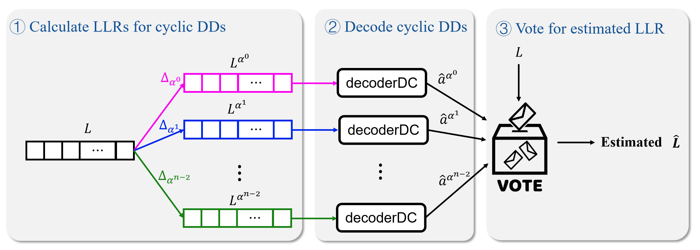
The algorithm takes $\bm{L}$ as an input and runs in an iterative manner. Let $B$ denote a collection of directions, i.e. a subset of $\mathbb{F}^{*}_{2^{m}}$, where $\mathbb{F}^{*}_{2^{m}}$ consists of all the nonzero elements in $\mathbb{F}_{2^{m}}$. As shown in Fig. 2, each iteration has three steps: 1) calculate LLR vectors of cyclic DDs for all $\beta\in B$; 2) decode all the cyclic DDs; 3) vote for the estimated codeword from the decoded descendant codewords.

1) The LLR vector associated with the cyclic DD in the direction $\beta$ is defined as

where $L_{i}^{\beta}$ is the LLR value associated with $\Delta_{\beta}A(\alpha^{i})=A(\alpha^{i}+\beta)-A(\alpha^{i})$. We calculate $L^{\beta}_{i}$ as

where $j$ satisfies $\alpha^{j}=\alpha^{i}+\beta$. We denote the procedure of calculating $\bm{L}^{\beta}$ with the input $\bm{L}$ and $\beta$ by $\bm{L}^{\beta}=\texttt{derivativeLLR}(\bm{L}\text{, }\beta)$.

2) According to Theorem 1, we can use the same decoder, denoted by decoderDD, to decode all the cyclic DDs. The decoding result of $\bm{L}^{\beta}$ is given by $\hat{\bm{a}}^{\beta}=\texttt{decoderDD}(\bm{L}^{\beta})$.

3) The final step is to use a soft-voting scheme to obtain a new LLR vector $\hat{\bm{L}}$. From (6), the “soft vote” from the estimate $\hat{a}_{i}^{\beta}$ to $L_{i}$ is $\widetilde{L}_{i}^{\beta}\triangleq(1-2\hat{a}^{\beta}_{i})L_{j}$. For the direction $\beta$, the “soft vote” from $\hat{\bm{a}}^{\beta}$ to $\bm{L}$ is given by

Here we have used the natural embedding of $\mathbb{F}_{2}$ in $\mathbb{R}$ for the interpretation of $\hat{a}^{\beta}_{i}$ in the above equation. Update $\bm{L}$ as the average of all the “soft votes” from different directions

Here, $\sum$ denotes the component-wise summation.

Once we update $\bm{L}$, we take $\hat{\bm{a}}=[\hat{a}_{i},i\in I]$ where $\hat{a}_{i}=\mathbbm{1}[L_{i}<0]$. If $\hat{\bm{a}}$ is a codeword in $\mathcal{C}$, i.e. $\mathbf{H}\hat{\bm{a}}^{\text{T}}=\bm{0}$ where $\mathbf{H}$ is the partiry-check matrix of $\mathcal{C}$ and $\hat{\bm{a}}^{\text{T}}$ denotes the transpose of $\hat{\bm{a}}$, we end the iteration and output $\hat{\bm{a}}$. Otherwise, proceed into the next iteration unless obtaining a codeword or reaching a maximal iteration number $N_{\emph{max}}$. The pseudo code of the above procedure is shown in Algorithm 1.

We analyze the computational complexity of the proposed algorithm per iteration according to Algorithm 1. Denote the code length by $n$. It takes $4n$ floating point operations to perform derivativeLLR. In each iteration, the decoder performs derivativeLLR and decoderDD $|B|$ times. At the end of each iteration, it needs $|B|n$ floating point operations for calculating the average of all the “soft votes”. Denote the number of floating point operation of decoderDD by $\Omega$. We get the following proposition.

Consider the $(64,24)$ eBCH code and the $(64,45)$ eBCH code. The corresponding generator polynomials in hexadecimal form are 0xF69AC20921 and 0x782CF, respectively. From (1), the corresponding representative sets are $S_{1}=\{0,1,3,5,9,21\}$ with $\texttt{deg}(S_{1})=3$ and $S_{2}=\{0,1,3,5,7,9,11,13,21,27\}$ with $\texttt{deg}(S_{2})=4$. According to Theorem 1, the representative sets associated with their cyclic DDs are $\{0,1,5\}$ and $\{0,1,3,5,9,11,13\}$. The corresponding codes are the $(64,13)$ extended EG code and a $(64,34)$ extended cyclic code. Please note that the $(64,34)$ extended cyclic code is a subcode of the $(64,37)$ extended EG code.

Consider additive white Gaussian noise (AWGN) channels. We decode the two eBCH codes by our proposed derivative decoding algorithm. The decoder for their cyclic DDs is the SPA decoder. The parity-check matrix used for decoding the $(64,13)$ extended EG code is a $336\times 64$ matrix with row weight $4$ and column weight $21$, and the one used for decoding the $(64,34)$ extended cyclic code is a $72\times 64$ matrix with row weight $8$ and column weight $17$. We set the maximum iteration numbers for SPA and DD as $N_{\emph{SPA,max}}=20$ and $N_{\emph{DD,max}}=3$, respectively. We perform derivative decoding in all the $63$ directions and denote the procedure by DD$(63)$-SPA. In addition, we perform derivative decoding in $16$ directions at random and denote the procedure by DD$(16)$-SPA. We compare with the performance of decoding BCH codes using the Berlekamp-Massey (BM) algorithm [5][20].

The simulation results are shown in Fig. 3 and the performance of the MLD is also provided. We see that at the block error ratio (BLER) of $10^{-4}$, DD$(63)$-SPA for the $(64,24)$ eBCH code and the $(64,45)$ eBCH code outperforms BM for the corresponding BCH codes about $2.9$ dB and $1.9$ dB, respectively. Moreover, the gaps between the MLD and DD$(63)$-SPA are $0.5$ dB and $0.3$ dB in, respectively. In addition, for decoding the $(64,45)$ eBCH code, DD$(16)$-SPA only performs about $0.2$ dB away from DD$(63)$-SPA at the BLER of $10^{-4}$.

Besides, we compare with the performance of decoding 5G CA-polar codes [21][22] with the same length and dimension. The decoder used for the CA-polar codes is the Successive Cancellation List (SCL) decoder[23] with list size $32$. And the CRC length is set to $6$. At the BLER of $10^{-5}$, DD($63$)-SPA for the $(64,24)$ eBCH code and the $(64,45)$ eBCH code outperforms SCL for the CA-polar codes with the same length and dimension about $0.4$ dB and $0.2$ dB, respectively.

We discuss the computational complexity of decoding the $(64,45)$ eBCH code using DD$(63)$-SPA. Denote the floating point operation cost of the SPA in one iteration by $\Omega_{\emph{SPA}}$. From Proposition 6, the number of the floating point operations is $320*63+63N_{\emph{SPA}}\Omega_{\emph{SPA}}$ per iteration where $\Omega_{\emph{SPA}}$ is the average iteration number of the SPA. At the $E_{b}/N_{0}$ of $5.0$ dB, the average iteration number of the SPA is $1.16$ and the average iteration number of DD$(63)$-SPA is $1.00$. As a result, the cost of DD$(63)$-SPA is around $20160+73\Omega_{\emph{SPA}}$ floating point operations. Besides, the average iteration number of the SPA in DD$(16)$-SPA and the average iteration number of DD$(16)$-SPA is also $1.16$ and $1.00$, respectively. Then the cost of DD$(16)$-SPA is around $5120+19\Omega_{\emph{SPA}}$ floating point operations.

Consider the RM code of length $2^{m}$ and order $r$ denoted by RM$(r,m)$. The zero set of the generator polynomial associated with RM$(r,m)$ is $\{\alpha^{j}:0<\texttt{wt}(\overline{j})<m-r\}$ [4, Chap. 6]. According to (1), the exponent set of RM$(r,m)$ is $\{j:0\leq\texttt{wt}(\overline{j})\leq r\}$. According to Theorem 1, we conclude that the cyclic DD of RM$(r,m)$ is RM$(r-1,m)$. Note that the dimension and minimum Hamming distance of RM$(r,m)$ are $\sum_{i=0}^{r}\binom{m}{i}$ and $2^{m-r}$, respectively. The equalities in Proposition 1 and Proposition 2 hold for RM codes and their cyclic DDs. Similarly, according to Proposition 3, we conclude that the cyclic DA of RM$(r,m)$ is RM$(r+1,m)$. The equalities in Proposition 4 and Proposition 5 hold for the RM codes and their cyclic DAs.

As a result, we can decode RM$(r,m)$ codes using derivative decoding based on the decodings of RM$(r-1,m)$ codes. Let $T$ denote a subset of $\mathbb{F}_{2^{m}}$ such that $(\beta+T)\cup T=\mathbb{F}_{2^{m}}$^†† For a subset $T$ of $\mathbb{F}_{2^{m}}$, $\beta+T$ denote the set $\{\beta+\alpha^{i}:\alpha^{i}\in T\}$.. From (2), we have $[\Delta_{\beta}A(\alpha^{i}),\alpha^{i}\in T]=[\Delta_{\beta}A(\alpha^{i}),\alpha^{i}\in\beta+T]$. Considering the $|\bm{u}|\bm{u}+\bm{v}|$-construction and the automorphism groups of RM codes[2, Chap. 13], we conclude that $[\Delta_{\beta}A(\alpha^{i}),\alpha^{i}\in T]$ is a codeword of RM$(r-1,m-1)$. The proof is given in the Appendix. From (6), we have $[L^{\beta}_{i},\alpha^{i}\in T]=[L^{\beta}_{i},\alpha^{i}\in\beta+T]$, where $[L^{\beta}_{i},\alpha^{i}\in T]$ is the LLR vector associated with $[\Delta_{\beta}A(\alpha^{i}),\alpha^{i}\in T]$. In other words, our derivative decoding derived from the MS polynomials can carry on based on the decodings of RM$(r-1,m-1)$ codes as the state-of-the-art projection decodings [14, 15] derived from the $m$-variate polynomials, and obtain the same performance.

If an extended cyclic code can be efficiently soft-decision decoded, then its cyclic DA can be soft-decision decoded by the derivative decoding algorithm. Consider the $(256,175)$ extended EG code with minimum Hamming distance 18 which can be efficiently decoded by the SPA decoder. The corresponding generator polynomial is 0x11377F7700FA55335BA55. The representative set of its exponent set is $S=\{0,1,3,5,7,9,11,13,17,19,21,$ $23,25,27,29,37,39,43,51,53,55,59,85,87,119\}$ with $\texttt{deg}(S)=6$. According to Proposition 3, we can construct its cyclic DA. It is an extended cyclic code of length $256$ and dimension $191\leq\sum_{i=0}^{7}\binom{8}{i}$ with distance $d\geq 18/2=9$, according to Proposition 4 and Proposition 5. In fact, this code, denoted by DA$(256,191)$ has minimum Hamming distance at least $16$ according to the BCH bound [4]. The corresponding generator polynomial of DA$(256,191)$ is 0x19ACCC1AE68A0CEFF.

In Fig. 4, we provide the simulation result of decoding DA$(256,191)$ using derivative decoding based on SPA with all the directions in $\mathbb{F}^{*}_{2^{m}}$, denoted by DD($255$)-SPA. The parity-check matrix used for decoding the $(256,175)$ extended EG code is a $272\times 256$ matrix with row weight $16$ and column weight $17$. The maximum iteration numbers for derivative decoding and SPA are set to $N_{\emph{DD,max}}=4$ and $N_{\emph{SPA,max}}=20$, respectively. The performance of the MLD is also provided. We see that at the BLER of $10^{-4}$, the gap between the MLD and DD-SPA is about $0.9$ dB.

Two codes are said to be equivalent [2, Chap. 1] if there is a permutation of the coordinates together with permutations of the coordinate values for each of the coordinates, that map the codewords of one code into those of the other. The following theorem proves that the minimal DDs in different directions are equivalent.

For an integer $b$, we make the agreement $\infty+b=\infty\text{ mod }n$. For a codeword $\bm{a}=[a_{i},i\in I]\in\mathcal{C}$, we define the $b$-cyclic shift of $\bm{a}$ as $\bm{a}^{(b)}\triangleq[a_{i+b},i\in I]$.

References

- [1] E. Prange, Cyclic error-correcting codes in two symbols. Air force Cambridge research center, 1957.
- [2] F. J. MacWilliams and N. J. A. Sloane, The theory of error correcting codes. Elsevier, 1977, vol. 16.
- [3] S. Lin and D. J. Costello, Error control coding. Prentice hall New York, 2001, vol. 2, no. 4.
- [4] R. E. Blahut, Algebraic codes for data transmission. Cambridge university press, 2003.
- [5] E. R. Berlekamp, Algebraic coding theory (revised edition). World Scientific, 2015.
- [6] A. Vardy and Y. Be’ery, “Maximum-likelihood soft decision decoding of BCH codes,” IEEE Trans. on Inf. Theory, vol. 40, no. 2, pp. 546–554, 1994.
- [7] N. Kamiya, “On algebraic soft-decision decoding algorithms for BCH codes,” IEEE Trans. on Inf. Theory, vol. 47, no. 1, pp. 45–58, 2001.
- [8] M. Bossert, R. Schulz, and S. Bitzer, “On hard and soft decision decoding of BCH codes,” IEEE Transactions on Information Theory, 2022.
- [9] X. W. T. L. Tapp, A. A. Luna and S. B. Wicker, “Extended Hamming and BCH soft decision decoders for mobile data applications,” IEEE trans. on commun., vol. 47, no. 3, pp. 333–337, 1999.
- [10] S. Lin, K. Abdel-Ghaffar, J. Li, and K. Liu, “A Scheme for Collective Encoding and Iterative Soft-Decision Decoding of Cyclic Codes of Prime Lengths: Applications to Reed-Solomon, BCH, and Quadratic Residue Codes,” IEEE Trans. on Inf. Theory, vol. 66, no. 9, pp. 5358–5378, 2020.
- [11] Y. Kou, S. Lin, and M. P. Fossorier, “Low-density parity-check codes based on finite geometries: a rediscovery and new results,” IEEE Trans. Inf. Theory, vol. 47, no. 7, pp. 2711–2736, Nov. 2001.
- [12] V. M. Sidel’nikov and A. Pershakov, “Decoding of Reed-Muller codes with a large number of errors,” Probl. Peredachi Inf., vol. 28, no. 3, pp. 80–94, 1992.
- [13] I. Dumer and K. Shabunov, “Soft-decision decoding of Reed-Muller codes: recursive lists,” IEEE Trans. Inf. Theory, vol. 52, no. 3, pp. 1260–1266, Mar. 2006.
- [14] M. Ye and E. Abbe, “Recursive projection-aggregation decoding of Reed-Muller codes,” IEEE Trans. Inf. Theory, vol. 66, no. 8, pp. 4948–4965, Aug. 2020.
- [15] M. Lian, C. Häger, and H. D. Pfister, “Decoding Reed-Muller codes using redundant code constraints,” in Proc. IEEE Int. Symp. Inf. Theory. IEEE, June 2020, pp. 42–47.
- [16] H. Mattson and G. Solomon, “A new treatment of Bose-Chaudhuri codes,” Journal of the Society for Industrial and Applied Mathematics, vol. 9, no. 4, pp. 654–669, 1961.
- [17] M. P. Fossorier and S. Lin, “Soft-decision decoding of linear block codes based on ordered statistics,” IEEE Trans. Inf. Theory, vol. 41, no. 5, pp. 1379–1396, 1995.
- [18] F. R. Kschischang, B. J. Frey, and H.-A. Loeliger, “Factor graphs and the sum-product algorithm,” IEEE Trans. Inf. Theory, vol. 47, no. 2, pp. 498–519, Feb. 2001.
- [19] R. Lucas, M. P. Fossorier, Y. Kou, and S. Lin, “Iterative decoding of one-step majority logic deductible codes based on belief propagation,” IEEE Trans. Commun., vol. 48, no. 6, pp. 931–937, June 2000.
- [20] J. Massey, “Shift-register synthesis and BCH decoding,” IEEE Trans. Inf. Theory, vol. 15, no. 1, pp. 122–127, Jan. 1969.
- [21] E. Arikan, “Channel polarization: A method for constructing capacity-achieving codes for symmetric binary-input memoryless channels,” vol. 55, no. 7, pp. 3051–3073, 6 2009.
- [22] “3GPP TS 38.212, 3rd Generation Partnership Project; Technical Specification Group Radio Access Network; NR; Multiplexing and Channel Coding (Release 16) V16.4.0 Technical Specification (TS),” Dec. 2020.
- [23] I. Tal and A. Vardy, “List decoding of polar codes,” IEEE Trans. Inf. Theory, vol. 61, no. 5, pp. 2213–2226, Mar. 2015.
- [24] R. C. Bose and D. K. Ray-Chaudhuri, “Further results on error correcting binary group codes,” Information and Control, vol. 3, no. 3, pp. 279–290, 1960.
- [25] ——, “On a class of error correcting binary group codes,” Information and control, vol. 3, no. 1, pp. 68–79, 1960.