Translationally Invariant Constraint Optimization Problems
Abstract
We study the complexity of classical constraint satisfaction problems on a 2D grid. Specifically, we consider the computational complexity of function versions of such problems, with the additional restriction that the constraints are translationally invariant, namely, the variables are located at the vertices of a 2D grid and the constraint between every pair of adjacent variables is the same in each dimension. The only input to the problem is thus the size of the grid. This problem is equivalent to one of the most interesting problems in classical physics, namely, computing the lowest energy of a classical system of particles on the grid. We provide a tight characterization of the complexity of this problem, and show that it is complete for the class . Gottesman and Irani (FOCS 2009) also studied classical constraint satisfaction problems using this strong notion of translational-invariance; they show that the problem of deciding whether the cost of the optimal assignment is below a given threshold is NEXP-complete. Our result is thus a strengthening of their result from the decision version to the function version of the problem. Our result can also be viewed as a generalization to the translationally invariant setting, of Krentel’s famous result from 1988, showing that the function version of SAT is complete for the class .
An essential ingredient in the proof is a study of the computational complexity of a gapped variant of the problem. We show that it is NEXP-hard to approximate the cost of the optimal assignment to within an additive error of , where the grid size is . To the best of our knowledge, no gapped result is known for CSPs on the grid, even in the non-translationally invariant case. This might be of independent interest. As a byproduct of our results, we also show that a decision version of the optimization problem which asks whether the cost of the optimal assignment is odd or even is also complete for .
1 Introduction
More than half a century ago, Cook and Levin inaugurated the field of NP-completness. The fact that the Constraint Satisfaction Problem (CSP) is NP-complete has been the cornerstone of our understanding and approach to important optimization problems arising in countless applications. The NP completeness of deciding whether a CSP instance is satisfiable, plays an important role also in physics. This is because constraint satisfaction corresponds to a classical local Hamiltonian which expresses the total energy of a system of particles; the energy is the sum of terms, each of which describes the energy interaction between constant-sized clusters of particles. Finding whether the lowest energy of such systems is below some threshold or above it, is a special class of CSP, and was famously shown to be NP-complete in many cases by Barahona and others [Bah82, Ist00]. The theory of NP-completeness has a natural generalization in the quantum setting; the Cook-Levin theorem was generalized by Kitaev [KSV02] to show that the following problem is QMA-complete: Given a local Hamiltonian with quantum energy interactions describing the energy in a quantum many-body system, decide whether the ground energy is above some value or below another; this problem has been intensely studied in recent years [KSV02, GHLS15, OT05, AGIK09].
A natural variant of the NP-complete decision CSP, is the function version of the CSP. In this version, the question is not whether all constraints can be satisfied, but what is the maximum number of constraints that can be satisfied by any assignment. One could also consider a weighted variant, as we do here, where the goal is compute the cost of the optimal assignment which minimizes the weighted sum of violated constraints. Computing the cost of the optimal solution is in fact the more natural version of CSP problems in a large number of combinatorial applications (to give just two examples, max-cut and max independent set). Importantly, in classical physics, when considering the local Hamiltonian corresponding to a CSP, the function version of the problem is in fact the problem of finding the lowest possible energy for the Hamiltonian over all possible states – one of the most important notions in physics. In the quantum case, the function version corresponds to providing an estimate of the lowest energy of the system over all possible quantum states, which is one of the main subjects of interest in condensed matter physics.
What is known from the computational complexity angle, about this physically motivated question, the function versions of CSPs? In 1988, Krentel [Kre86] proved that the function problem for constraint satisfaction is -complete. Krentel’s proof is significantly more involved technically that that of the Cook-Levin’s theorem which characterizes the complexity of the decision variant of CSPs. Furthermore, and in stark contrast to the theory of decision problems and NP-completeness, the function version of CSP seems to have received less attention in the TCS literature.
From the physics point of view, an additional point becomes extremely important. By and large, physicists study local Hamiltonians, be them classical or quantum, in a translational-invariant (TI) setting. In this setting the particles are located at the vertices of a geometric lattice and all the terms acting on adjacent pairs of particles along a particular dimension are the same. In particular, the model most relevant to physics is TI in a very strong sense: the dimension of the individual particles and the Hamiltonian term acting on each pair of adjacent particles in a lattice are fixed parameters of the problem. When considering finite systems, the only input is an integer indicating the size of the system. This set-up corresponds to the fact that in physics, different Hamiltonians represent completely different physical systems. Thus, studying the ground energy (or some other quantity) in the AKLT model is considered to be a completely different problem than studying the same quantity in, say, the Ising model 11 1 Some of the recent work on the quantum TI local Hamiltonian problem [BCO17] adopt a weaker notion in which the input also includes the Hamiltonian term that is applied to each pair of particles, allowing the Hamiltonian to be tuned to the size of the system. This model is mainly considered in quantum Hamiltonian complexity, but have not been a topic of study in physics..
For decision problems, Gottesman and Irani [GI13] show hardness results for both quantum and classical TI Hamiltonians. Since the size of the grid can be given by logarithmically many bits, and there is no other input, one encounters an exponential factor compared to the common CSP problems; thus the results in [GI13] show NEXP and completeness for the classical and quantum variants of the problem, respectively. We note that a tightly related line of works studies TI infinite systems [AI21, WC21, CPGW15] and considers computability and computational complexity of decision problems in that domain, namely in the so called thermodynamic limit. Although the focus here is on finite systems, constructions for finite systems have played an important role for the results in the thermodynamic limit. In particular, all the results in [AI21, WC21, CPGW15] use a finite construction layered on top of a certain type of aperiodic tiling of the infinite grid.
To the best of our knowledge, the computational complexity of function CSPs in the TI setting, has remained open. In this paper we provide a tight characterization of its complexity, and show that the function version of TI CSP on a -dimensional grid is complete for . This result thus strengthens Krentel’s construction for general CSPs to apply even TI systems for two and higher dimensions. The result is also a generalization of Gottesman-Irani who prove hardness for 2D TI systems for the standard decision problem, where one only needs to determine if the ground energy is below a given threshold. One of the key technical challenges in our result is to effectively create large () costs on an grid using only two constant-sized terms which apply in the horizontal and vertical directions. Thus, as a stepping stone to the more complex result on the function version of TI 2D CSPs, we show a fault-tolerant result which we believe is of interest on its own, namely that it is NEXP-complete to even approximate the ground energy to within an additive .
1.1 Problem Definitions, Results and Main Challenges
It is most convenient to present our results using the language of the weighted tiling problem, where we focus here on the two dimensional case22 2 Our version of tiling is equivalent to the more common Wang tiles [Wan60].. In this tiling problem, one is asked to tile an 2D grid with a set of tiles. The tiles come in different colors and only some pairs of colors can be placed next to each other in either the horizontal or vertical directions. More precisely, a set of tiling rules is a triple , where is a finite set of tile types , and and are functions from to . For , is the cost of putting a tile of type immediately to the left of a tile of type and is the cost of putting a tile of type immediately above a tile of type . Let be the minimum cost of tiling an grid with tiling rules . The goal is to tile the grid with minimal total cost. Note that this problem is directly analogous to a classical Hamiltonian in 2D. We first define a function version of the problem.
Definition 1
-FWT (Function Weighted Tiling)
Input: An integer specified with bits
Output:
Theorem 1.1
(Main) There exists a set of tiling rules such that -FWT is -complete.
We note that the fact that the function problem is complete for 2D immediately implies that it is complete for any grid of dimension at least since the 2D construction can be embedded into a higher dimensional grid. The 1D CSP case is poly-time computable using dynamic programming.
The upper bound in Theorem 1.1 is easy: it can be achieved by binary search with access to an oracle for the decision problem. For the lower bound, one encounters a challenge. The reduction must encode in the tiling rules the computation of a polynomial time Turing Machine with access to a NEXP oracle. If an instance given to the oracle is a yes instance, the computation of the verifier can be encoded into the tiling rules. However no instances cannot be directly verified in this way. Krentel’s proof that the function problem of weighted SAT is -complete [Kre86] overcomes this challenge; let us recall it and then explain the problem in carrying it over to the TI setting. Krentel uses an accounting scheme [Kre86, Pap94] that applies a cost to every string representing guesses for the sequence of responses to all the oracle queries made. The accounting scheme needs to ensure that the minimum cost is equal to the correct sequence of oracle responses, . yes and no guesses are treated differently, due to the fact that the verifier can check yes instances (and thus incorrect yes guesses can incur a very high cost), but no guesses, cannot be directly verified. In Krentel’s scheme, no guesses incur a more modest cost, whether correct or not, and their cost must decrease exponentially. This is because the oracle queries are adaptive; an incorrect oracle response could potentially change all the oracle queries made in the future and so it is important that the penalty for an incorrect guess on the query is higher than the cost that could potentially be saved on all future queries. The weights on clauses that implement this accounting scheme are multiplied by a large power of two to ensure that they are the dominant factor in determining the optimal assignment.
The difficulty in applying Krentel’s accounting scheme in the TI setting is that the costs must grow with the size of the input. Therefore, it is not possible to apply the costs directly into the tiling rules which are of fixed constant size. A natural attempt to circumvent the problem is to assign the required large penalty by many tiles, each of which would acquire a constant penalty; however, the problem in implementing this approach is that Cook-Levin type reductions from computations to tilings are very brittle, as a single error can potentially derail the entire computation. For example, imagine inserting a row that does not have a Turing Machine head. There will be a single fault where the head disappears from one row to the next, but every row thereafter will contain the unchanging contents of the Turing Machine tape without a head to execute a next step. This imposes a challenge since when enforcing large costs by using many tiles, or constraints, we need to make sure that many of these constraints are indeed violated in order to incur the required large penalty.
We provide a construction which circumvents this issue by exhibiting some fault tolerance properties. We thus prove what can be viewed as a gapped version or a hardness of approximation result, which is then a natural stepping stone to implementing the more intricate function required in Krentel’s accounting scheme. To this end we define an approximation version of weighted tiling:
Definition 2
-GWT (Gapped Weighted Tiling)
Input: An integer specified with bits. Two integers and such that .
Output: Determine whether or .
Theorem 1.2
There exists a set of tiling rules such that -GWT is NEXP-complete for a function .
This shows that it is NEXP-hard to even approximate the cost of the optimal tiling to within an additive error that is . This can be viewed as a gapped version of the results of [GI13]; the proof constructs a reduction mapping the computation into a tiling such that even in the presence of faults, the computation encoded by the tiling is able to proceed and produce approximately correct results.
Theorem 1.2 is of potential interest on its own. It might resemble a PCP type result, but the model we consider differs from the standard PCP setting in two ways: the first is that the underlying graph is a grid, rather than a graph with much higher connectivity, and the second is translational-invariance. It is not possible to obtain a hardness of approximation result with an additive error that is linear in (as one has in the PCP theorem) on any finite dimensional lattice because such graphs do not have the necessary expansion properties. For example, in 2D, one could divide the grid into squares for and solve each square optimally in polynomial time. The resulting solution would be within an additive of the optimal solution. To the best of our knowledge, no gapped version was proven before for CSP problem set on a constant dimensional grid, even without the TI restriction.
Finally, our results provide tight characterizations of the complexity of the following decision problem;
Definition 3
-PWT (Parity Weighted Tiling)
Input: An integer specified with bits
Output: Determine whether is odd or even.
The proof is very similar to the proof of Theorem 1.1. The result on Parity Weighted Tiling illustrates that decision problems related to CSP can be complete for an oracle class just like the function problem. The crucial difference between the threshold decision problem (is the cost of the optimal solution less than ?) which is NEXP-complete and the parity problem which is -complete is that the parity problem still seems to require determining the optimal cost. This seems to make the characterization of its complexity as challenging as for the function version of the problem.
1.2 Tiling Rules and Layers
We assume that there is a special tile denoted by which must be placed around the perimeter of the grid to be tiled. Moreover, no tile can be placed in the interior of the grid. We will return later to enforcing this condition in the context of the different problems. The tiles on the interior will be composed of multiple layers where each layer has its own set of tile types. A tile type for an internal tile in the overall construction is described by a tile type for each of the layers.
For ease of exposition, we allow our tiling rules to also apply to local squares of four tiles. This can easily then be translated to two-local constraints on tiles, as in our definition of the tiling problem. This simple transition is described more fully in Section 2.1. For the remainder of the paper our tiling rules include constraints on local squares of four tiles, as well as pairs of horizontal tiles.
If the four tiles in a square are all interior tiles, then each possible pattern of four square tiles within a layer will be designated as legal or illegal. The overall cost of placing four interior tiles in a local square together will be function of whether the square for each layer is legal or illegal. For the Gapped Weighted Tiling, the cost will be just the number of layers for which the square pattern is illegal. For the Function Weighted Tiling and Weighted Tiling Parity, illegal squares at different layers will contribute different amounts to the cost.
In general, a no-cost tiling of each Layer represents a computational process where each row represents the state of a Turing Machine. The computation reverses direction from one layer to the next. The rows of a tiling of an grid will be numbered through from bottom to top. When referring to the rows in a particular layer, we will exclude the border rows and order the rows according to the computation direction. So the first row of Layer , which proceeds from bottom to top, is row and the last row of Layer is . Layer proceeds from top to bottom, so the first row for Layer is and the last row is .
For the most part, the rules governing the tiling apply to the tile types within each individual layer. The different layers only interact at the lower and upper border of the grid. This is how the output of one process (on Layer ) is translated into the input for the next process (on Layer ). For example, a square may be illegal if the two lower tiles are , and the two upper tiles violate certain constraints between the Layer and Layer types. Some of the layers will also have additional constraints on which tiles can be next to each other in the horizontal direction. Each type of violated constraint is given a name described below.
Definition 4
[Faults in a Tiling] An occurrence of any of the illegal patterns described in the constructions is called a fault. A tiling with no faults, will correspond to a fault-free computation.
There will be some additional costs (described later) associated with a computation ending in a rejecting state. These are not considered faults because they can happen in correct computations. Figure 1 illustrates the different types of tiling constraints.
-
Illegal Computation Squares: For each layer, every pattern of four tile types will be designated as a legal computation square or an illegal computation square. In general, these rules enforce that the tiling within the layer represents a consistent execution of a Turing Machine. We describe in Subsection 2.2 how to translate the rules of a Turing Machine into legal and illegal computation squares.
-
Illegal Pairs: Some of the layers will have additional constraints on which tiles can be placed next to each other in the horizontal direction. Each ordered pair of tiles types for that layer will be designated as a legal pair or an illegal pair.
-
Illegal Initialization Squares: For each layer, there are also some initialization rules that constrain the initial configuration of the Turing Machine. If the layer runs bottom to top, then these rules apply to , which consists of all tiles, and the first row of the layer. For example, if tile can not be immediately to the left of in the first row of Layer , then the square with directly below is an illegal initialization square for Layer . If the Turing Machine for the layer runs top to bottom, then the square with directly above in Layer is illegal.
-
Illegal Translation Squares: Finally, we add rules that control how the last row of Layer is translated to the first row of Layer . If Layer runs top to bottom, then the rules apply to rows and . For example, if tile in Layer cannot be translated to in Layer , then any square with a directly below a tile whose Layer type is and whose Layer type is would be illegal. The translation rules can also apply to pairs of adjacent tiles. E.g., it could be illegal to have a square whose bottom two tiles are and whose top two tiles have in Layer and in Layer .


1.3 Proofs Overview
Thoeorem 1.2: Gapped Weighted Tiling Recall that the standard encoding of a Turing Machine into tiling rules is very brittle in that a single fault can derail the entire computation. The most straight forward way to overcome this is using a construction which embeds many repetitions of the computation, so that many faults would be required to derail a large number of those computations. Multiple computations thus need to be set up and initiated, using a single faulty Turing machine with TI rules. In our construction, this is achieved by a first stage of the computation (implemented in Layer , as we describe below), which, roughly, creates intervals in the top row of Layer , such that the independent repetitions of the computations will occur in different strips on the grid; the boundaries of the strips are determined by those intervals. The difficulty is how to implement the initial set up using a single Turing machine, in a fault tolerant way. We now describe the details.
The tiling rules for the first two layers, as well as the reduction mapping to are independent of the language , the language we are reducing from. Let denote the exponential time verifier for . Subsection 2.2 describes the details of how a Turing Machine computation is encoded in a set of tiling rules. In general tiles will be either tape tiles which encode a single symbol from the Turing Machine’s tape alphabet or head tiles which encode both the state of the Turing Machine as well as the current tape symbol to which the head is pointing.
The Turing Machine computation represented in Layer starts with two non-blank symbols and proceeds to write a sequence of intervals on the tape, where an interval is a sequence of symbols bracketed on either side by a delimiter tile from the set . The Turing Machine just repeatedly executes a single loop which we refer to as the Outer Loop. In one iteration of the Outer Loop, an additional symbol is inserted into every interval and a new interval with no ’s in the middle is added to the right end of the non-blank symbols. In an fault-free execution of the Turing Machine, after iterations of the loop, there are intervals. The number of symbols in each interval (including the delimiter tiles on either end) is . For , the row should look like:
| B | B | B | X | B | B | X | B | X | # | # | # |
When the top row of Layer 1 is translated to Layer , the head tile for the Layer Turing Machine is translated to a tape tile (so the state information is lost) and a head tile is inserted on the left end of every interval. For example, an interval at the end of Layer is translated to in the first row of Layer . In Layers and the sizes and locations of the intervals do not change within a row unless the interval contains an illegal square. Thus, a single interval over all the rows of Layer forms a vertical strip of tiles, and a separate, independent computation takes place within each strip. See Figure 7 for an example. Once the intervals are created on Layer , each computation on Layers and is fault-free unless the strip contains an illegal square. Thus, the number of illegal squares is at least the number of strips that fail to complete their computation correctly.
In Layer , the computation is just a binary counter Turing Machine that continually increments a binary counter. All the strips that do not contain an illegal square will have the same string represented in the final row of Layer . The string then serves as the input to the computation in Layer . The binary counter Turing Machine in Layer runs for exactly steps. The reduction is the function that maps to , where the string is written on the tape of a binary counting Turing Machine after steps. Lemma 5.3 gives an exact formula mapping to and shows that the value of the number represented by the string is , the dimension of the grid. The idea of using a binary counting Turing Machine to translate the size of the grid to a binary input for a computation was used previously in [GI13]. Although since the construction in [GI13] had a gap of , only a single execution of the verifier was needed. Since we are trying to produce a gap of , we need at least separate computations each of which simulates the verifier on input .
Each interval is translated unchanged to Layer . The computation in each strip in Layer simulates the verifier on input using a witness that is guessed in the tiling. There is a final cost for any rejecting computation. If , it will be possible to tile each strip at cost. If , every strip will contain an illegal square or will incur a cost for the correct rejecting computation. Thus, the gap is essentially created by these parallel computations, each of which contributes a constant cost if .
Since the sizes of the intervals go down to , some of the intervals will be too narrow to complete the computation in either Layers or . If the head ever hits the right end of its interval, it transitions to an infinite loop, causing no additional cost. A standard padding argument (Claim 5.1) guarantees that an interval need only be wide to complete the computations in Layers and . The analysis of Layer then needs to guarantee that despite the faults, there will be sufficiently many sufficiently wide intervals.
The main challenge in the proof is in making the computation in Layer fault-tolerant, meaning that each illegal pair or square cannot derail the computation too much. The horizontal rules in Layer are critical for enforcing that this cannot happen. We show that a row in the tiling that has no illegal pairs corresponds to a sensible configuration of the Turing Machine. In particular such a row has exactly one head tile that lies in between the and tiles. Note that faults can still alter the computation in potentially strange ways. Nonetheless, we also show that starting from a row with no illegal pairs, the Layer Turing Machine will be able to make progress, and after a sequence of fault-free steps (corresponding to a sequence of rows containing no illegal squares), the computation will perform a complete iteration of the loop. Since the number of illegal pairs and squares is bounded by , there are enough complete iterations of the loop to ensure that the last row of Layer has enough intervals that are wide enough to complete the computations in Layers .
By far the most technically involved part of the paper is the analysis of Layer described in Section 4. All of the results use the final Lemma 4.23, which gives a tight characterization of the difference between the final row in Layer of a fault-free tiling and the final row of a tiling with faults. In fact, the result on Gapped Weighted Tiling could be established with looser bounds, but we provide the analysis once in Section 4 in a form that can be used for all the results in the paper. Section 1.3 describes more fully how this tight characterization is accomplished. A more in-depth overview is then given in the beginning of Section 4.
Theorem 1.1: Weighted Tiling Function The hardness reduction for Function Weighted Tiling reduces from an oracle class. The function is computed by a polynomial time Turing Machine with access to an oracle for language . Let denote the exponential time verifier for . Using a standard padding argument (see for example Lemma 2.30 from [AI21]) we can assume that for a constant of our choice, for every , there is a , such that the size of is at most , and M makes at most oracle calls to . Let denote an -bit string denoting the responses to the oracle queries made on input . With and fixed, the set of inputs to the oracle is also determined. is an indicator function denoting whether is in . Note that since is in NEXP, if , there exists a witness that will cause the verifier to accept and if , V will always reject regardless of the witness. Define:
Let be the output of Turing Machine on input with oracle responses . Note that since , . The construction will ensure that the minimum cost tiling for a particular and will be Note that represented in the high-order bits of the cost has the necessary structure where the costs for a no oracle response decrease exponentially in , the index of the oracle query. The cost for a yes guess will be if the input to the oracle is in fact in (i.e., ) and will be a very large cost of if is not in . This function will guarantee that the overall cost is minimized when is the correct string of oracle responses. In addition, the low order bits encode the output of the function . So if the minimum cost tiling can be computed, this will correspond to , which is , where is the string of correct oracle responses. The factor of ensures that even if the minimum cost is off by , the value of can still be recovered.
So far what we have described just implementing the original accounting scheme devised by Krentel. The challenge is to implement this cost function in 2D with TI terms. Note that since the tiling rules are fixed parameters of the problem, it is not possible to encode the cost function directly into the penalty terms. As with the Gapped Weighted Tiling problem the function is collectively computed by a set of parallel processes within each strip created by the intervals from Layer . However, instead of a threshold function which is either or , the parallel processes must collectively compute the more intricate function described above, which requires that the individual processes have some additional information.
We will describe first what happens in a fault-free computation (with no illegal pairs or computation squares) and then describe how fault-tolerance is enforced and proven. The construction for Layers and are exactly the same as for the Gapped Weighted Tiling problem. Layer creates a set of intervals. We definite the function to denote the number of intervals on the tape if the Turing Machine for Layer executes steps. If after steps, the computation just happens to finish at the end of an execution of the Outer Loop then the intervals have sizes (from left to right) . If the computation finishes in the middle of an execution of the Outer Loop, the actual sequence of interval sizes will be close to . The largest interval could have size and there may be a couple missing values in the range where the current interval is being increased. Lemma 4.24 describes the possible deviations in detail. is and we show using a standard padding argument that for the constant of our choice, all of the computations require at most space. This allows us to establish that at least half of the intervals will be large enough to complete the required computations.
As in the previous construction, Layer then executes a binary counting Turing Machine which results in the string written to the left of each interval which is large enough to complete the computation. Note that Layer is a global Turing Machine which executes a single process across the entire grid, while Layer represents local computations within each strip. When is translated from Layer to Layer it is augmented with a guess string for the oracle queries. . However, there is no guarantee that the guess for each interval is the same. Note that can be arbitrary but it must be consistently the same for each interval. Layer then executes a global Turing Machine which imposes a high penalty if the strings in each strip are not all the same. This penalty is higher than the cost function for any , so the lowest cost tiling will correspond to a configuration in which each strip has the same and .
Finally, in Layer , there is a local computation in each interval, each of which makes a or contribution towards the overall cost. The computation within each interval requires a unique tag in order to determine which term of the cost it will contribute to. The tag comes from the size of the interval. The computation begins with counting the number of locations in the interval. This can be accomplished by having the head shuttle back and forth between the two ends of the interval implementing both a unary and binary counter until the unary counter extends across the entire interval. The head returns to the left end of the interval and begins the next phase of the computation. Since the size of an interval is at most this phase of the computation will take at most steps.
Now each computation has the same pair and a its own integer indicating the size of the interval. From , the values of and can be determined. Lemma 4.24 shows that in a fault-free computation, the sizes of the intervals will decrease from left to right. Moreover, all interval sizes are in the set with at most one missing value from that set and at most two duplicates. Thus, the value , will be an almost unique identifier for each interval, starting with or on the left and increasing to the right. Using this tag, each interval determines which portion of the cost it will contribute to. The number of intervals assigned to compute a particular term in the cost will depend on the value of the term since each interval can contribute at most to the overall cost. If an interval is assigned to check a yes guess () the computation uses and to determine the input to the oracle , guesses a witness and simulates on input with the guessed witness. There is a cost of if rejects and if accepts. If is in fact in , there is a witness which will allow for a zero cost tiling withing that interval. If , then every witness will lead to a cost. Thus, the optimal set of witnesses will result in the minimum value for . In addition, exactly of the intervals will just transition to the rejecting state, incurring a cost of . The total cost due to those intervals is . For the remaining intervals, no cost is incurred.
The cost of a computation fault (illegal pair or square) is a constant that is larger than the cost of ending in a rejecting computation. Therefore, for each independent computation (in Layers and ) the optimal tiling will correspond to a correct computation which may or may not incur a cost for ending in a rejecting state. Technically, the most challenging part of the proof is to show that the process on Layer which creates the intervals is fault-tolerant. The proof for Function Weighted Tiling requires stronger conditions than for Gapped Weighted Tiling since we not only have to show that there are a large number of large intervals at the end of Layer but we need to establish that the sequence of interval sizes is close to what one would have in a fault-free computation. To this end, we use a potential function which captures how much a sequence of interval sizes deviates from the expected sequence . The main part of the proof is to show that each illegal square or pair can cause the value of to increase by at most a constant amount. At the end of Layer , the ideal sequence of interval sizes is . Every interval size that is missing from the actual sequence of interval sizes has caused to increase by at least a fixed amount which in turn corresponds to faults incurred in the computation. Thus, we show that it is more cost-effective to complete the computation correctly (and not incur the higher cost of a fault) and incur the smaller potential cost of a rejecting computation.
The most important measure of progress of the tiling/computation in Layer is the number of times the encoded Turing Machine completes an iteration of the Outer Loop in which the size of every interval increases by and a new interval of size is added. Faults can potentially cause an iteration of the Outer Loop to take longer as they may force the head to shuttle back and forth more times which in turn could result in fewer iterations. Even in a fault-free computation, the number of steps per iteration increases with each iteration because there are more intervals. One of the main lemmas in the analysis is Lemma 4.10 which lower bounds the number of times the loop is completed in relation to that number in a fault-free computation. The proof is a delicate inductive argument which uses the fact that the increase in the running time of a loop is not accelerated too much with each additional fault.
Proof Overview for Parity Weighted Tiling The proof for parity weighted tiling is very similar to the function problem. Suppose that a language is computed by a Turing Machine with access to an oracle for . Let be the indicator function that is if accepts and if rejects. The overall cost computed by the collective computations is: . The left-most interval computes and results in a cost in the case that rejects. The remaining intervals which collectively compute Krentel’s cost function all impose costs of or . Thus the expression will guarantee that the minimum corresponds to the correct guess . Furthermore, the rightmost bit will be which will cause the minimum cost to be odd or even, depending on whether accepts.
1.4 Discussion, Related Work, and Open Problems
Despite the fact that the function version of classical local-Hamiltonians describes the task of the computational (classical) physicist much more naturally than decision problems, complexity of function problems was hardly studied even in the non-TI setting, in the literature of classical theory of computer science.
Recently, related results were discovered in the domain of quantum computational complexity. In particular, in [AI21], Aharonov and Irani use a construction for the function version of (finite) quantum local Hamiltonian as a component for a hardness result for the infinite 2D grid. More specifically, they prove that the problem of estimating the ground energy of a local Hamiltonian on a finite 2D grid, is hard for . Importantly, their results do not imply the hardness result presented in this paper, and it seems impossible to extend their proof to deduce the classical hardness result of Theorem 1.1. Like [AI21] we implement Krentel’s cost function using a fixed Hamiltonian term, but since their construction is quantum (as opposed to the classical construction in this paper), they are able to prove the result using a completely different set of tools which do not carry over to the classical case. In quantum constructions, the lowest energy is an eigenvalue of a general Hermitian matrix and the matrix can be constructed to fine tune the ground energy to an inverse polynomial precision. In classical constructions, the total energy will be a sum over terms where each term is chosen from a constant-sized set of values determined by the finite horizontal and vertical tiling rules. This allows far less control in the classical setting over the precision of the minimum cost tiling.
Incidentally, note that the results for the quantum case proven in [AI21] are not tight, which follows from the fact that they use a quantum construction to obtain hardness for , a classical complexity class. It seems challenging to make the characterization tight in the quantum case. In contrast to the class NP, the class QMA is a class of promise-problems and in simulating a machine, there is no guarantee that the queries sent to the QMA oracle will be valid queries. The cost/energy applied for a particular query will depend on the probability that a QMA verifier accepts on the provided input. If the input is invalid, then the probability of acceptance can be arbitrary. Thus, Krentel’s cost function will potentially be an uncontrolled quantity. Typically in a reduction where we want to embed the output of a function into the value of the minimum energy, the low order bits of the energy are used to encode the output of the function. It’s not clear how to do this without being able to control the binary representation of the minimum energy. Note that by embedding a classical computation in the Hamiltonian, the issue of invalid queries is circumvented.
Both [AI21] and [WC21] study the complexity of computing the ground energy density of infinite TI Hamiltonians to within a desired precision making use of the technique introduced by Cubitt, Prerez-Garcia, and Wolf which embeds finite Hamiltonian constructions of exponentially increasing sizes, into the 2D infinite lattice, using Robinson tiles. Robinson tiling rules [Rob71] force an aperiodic structure on the tiling of the infinite plane, with squares of exponentially increasing size. The quantum construction of [AI21] layers a TI 1D Hamiltonian on top of one of the sides of all the squares. The classical construction of [WC21] layers a classical finite construction on each square. Neither work obtains tight results due to the same issue with invalid queries, although the two papers compromise in completely different ways. The primary technical innovation introduced in [WC21] is to devise a more robust version of Robinson tiles which ensures that the lowest energy state corresponds to a correct Robinson tiling, even though the cost of the classical finite construction layered on top may introduce a penalty. If it were possible to obtain an even more robust version of Robinson tiles, one potentially could layer the finite construction from the current paper on top the more robust constructions in the hopes of showing that computing the ground energy density of a classical TI Hamiltonian in the thermodynamic limit is complete for under Karp reductions.
The results in this paper are also related to the work of Ambainis [Amb14] which characterizes the complexity of measuring local observables of ground states of local Hamiltonians (APX-SIM), showing that the problem is complete for . contains those problems that can be solved by a polynomial time classical Turing Machine with access to queries to a QMA oracle. This type of question (determining a property of the ground state) is similar to our classical result about determining whether the cost of the optimal tiling is odd or even. The results on APX-SIM [Amb14, GY19, GPY19] are not hindered by the issue of invalid queries because the quantity being measured is not the actual energy itself. Note that the important point here is the property that distinguishes the state to be measured (minimum energy) is different than the local observable applied to the measured state. By contrast, computing the energy of the lowest energy state appears to be more difficult. The issue of invalid queries appears to be an obstacle, even when the Hamiltonian terms are position-dependent as in the constructions of [GY19, GPY19], as well as in the TI constructions in [AI21, WBG20].
Finally, it was mentioned earlier that the approximation problem considered here differs from the standard PCP setting in that the underlying graph is a grid and the terms are TI. It remains an open question as to whether there is a family of TI instances of constraint satisfaction on general graphs for which it is hard to estimate the optimal solution to within an additive .
1.5 Paper Outline
Section 2.2 describes how the rules of a Turing Machine are translated into tiling rules. For all the results presented here, Layer encodes the execution of a Turing Machine that creates intervals within the grid that marks off where parallel computations will take place in subsequent layers. Since the construction and analysis is common to all the results, we present that first. Section 3 gives the construction and Section 4 proves the main lemmas that are needed for the analysis of each construction. Section 5.2 then describes the rest of the construction and proof for Gapped Weighted Tiling which only requires two additional layers. Section 7 describes the rest of the construction and analysis for Parity Weighted Tiling. Finally, Section 6 describes the modifications to the construction for Parity Weighted Tiling that is requires for Function Weighted Tiling.
2 Tilings and Turing Machines
2.1 Equivalence of Tiling Variants
We defined the translationally-invariant tiling problem to use two constraints: one is applied to each pair of adjacent tiles in the vertical direction and the other is applied to each pair of adjacent tiles in the horizontal direction. For convenience, the local constraints described throughout the paper apply to local configurations in a square of four tiles as well as to pairs of tiles in the horizontal direction.
We sketch here how one can transform a set of a set of tiling rules that applies to squares into an equivalent one that applies to only pairs. For each pair of tiles and in the original tiling rules, create a new combined tile type . A large (but constant) constraint can be added to ensure that a tiling with the new tile types is consistent, meaning that a tile of the form must go to the left of a tile of the form . More specifically, an inconsistent tiling can be transformed into a consistent tiling in a way that strictly reduces the cost.
There is now a one-to-one correspondence between consistent tilings with the new tile types and tilings with the original tile types. Moreover, a vertically aligned pair with tile on top of can enforce the same constraint as a square in the original tiling rules with tiles and in the top row of the square and with and in the bottom row of the square. Constraints on the new tiles can be fixed so that the cost of corresponding tilings are the same.
2.2 Encoding Turing Machine Computations in Tilings
In this subsection we describe how the rules of a Turing Machine are translated into legal and illegal computation squares so that a tiling that contains no illegal computation squares corresponds to a correct execution of the Turing Machine. Note that the illegal and legal computation squares described in this subsection would apply to one particular Layer of the tiling. We assume here that the Turning Machine proceeds from the bottom to the top. If the direction were reversed, the the top and bottom rows of the legal and illegal computation squares would be swapped.
Consider a Turing Machine with tape alphabet and set of states . The set of tiles types for the layer corresponds to . A tile is called a tape tile if it is labeled with a symbol from the tape alphabet. A tile is called a head tile if it is labeled with a state and tape alphabet symbol, e.g. .
Each configuration of the Turing Machine is represented by a row of tiles. In general, we will have Turing Machines whose non-blank tape symbols are bracketed on the left by the symbol and on the right by symbol . The tape contents to the right of is an infinite sequence of blank () symbols. The corresponding row of tiles will have tiles extending to the tile at the right side of the grid. For example, consider a Turing Machine with state and whose tape symbols include B, X, , and . The Turing Machine configuration
-
B B B B X B B B X B X
will be represented by the row
| B | B | B | B | X | B | B | B | X | q/B | X | # | # | # |
For ease of notation, we will represent this row of tiles by the string:
Suppose the Turing Machine has rule then the following four squares would be legal for any tape symbols and :
| b | |
| x |
| b | y |
| y |
| y | |
| y | x |
| x |
Thus if two adjacent rows do not contain any illegal computation squares, then the next row up reflects the head location and tape contents after the rule has been applied.
Similarly, if the Turing Machine has rule then the following four squares would be legal for any tape symbols and :
| b | |
| x |
| y | b |
| y |
| b | |
| y | |
| x | y |
There can also be Turing Machine rules in which the head does not change location: . Then the following three squares would be legal for any tape symbol :
| x | |
| x |
| x | |
|---|---|
| x |
In the absence of a head tile, two vertically neighboring tiles must be the same tile type. Thus for any two tape symbols and the following square is legal:
| x | y |
| x | y |
All squares that have four interior tiles and whose tile types for the layer are not one of the legal squares described above is an illegal computation square.
In general, we will design TMs where each state is reached from a unique direction. In other words, for each state , the TM can not have rules corresponding to more the one of the following three forms:
- 1.
- 2.
- 3.
Any TM that doesn’t have this property can be transformed into a TM that does have this property by adding some additional states and rules. This restriction ensures that for each state , and any tape symbols , , and , only one of the squares below can be legal:
| y | |
| y | x |
| y | |
| x | y |
| y | |
| y |
Thus the only legal way for a head tile to appear in a row, is for there to be another head tile just below it or to the immediate left or right in the preceding row.
Definition 5
The number of illegal pairs and squares in Layer , denoted by is the number of illegal pairs, illegal computation squares, and illegal initialization squares in Layer , plus, if , the number of illegal translation squares from Layer to Layer . We will refer to as the cost of Layer .
The cost of the whole tiling will be a linear combination of the ’s.
A square is called a a head square if one of the two lower tiles is a head tile and one of the two upper tiles is a head tile. Note that a head square can be illegal or legal. The next two facts about the encoding of Turing Machines in tiling rules will be useful in analyzing Layer 1 of the constructions. Based on the method described above for translating Turing Machine rules into legal and illegal computation squares, the following two sets of facts can be easily verified.
Fact 2.1
Consider a tiling where a tile is directly above tile . If any of the following conditions hold, then both squares containing and are illegal computation squares:
- 1.
and are both tape tiles and
- 2.
is a head tile , is a tape tile and .
- 3.
is a tape tile , is a head tile and is not a TM rule.
- 4.
is a head tile , is a head tile and is not a TM rule.
Fact 2.2
Consider a tiling where a tile is directly above tile . If either of the following two conditions hold, then the vertically aligned pair is in a legal head square or an illegal computation square
- 1.
is a head tile , is a tape tile and .
- 2.
is a tape tile , is a head tile and is a valid TM rule.
- 3.
is a head tile , is a head tile and is a TM rule.
3 Layer 1 Construction: Creating the Intervals
3.1 Overview of Layer 1
The role of Layer 1 is to create what we call ”intervals” whose beginning and ends will mark the regions where separate computations which we want to repeat in the next layer, can occur.
We will refer to an interval as a sequence of characters that start with a heavy tile from the set and includes all the ’s to the right, up to and including the next heavy tile so that neighboring intervals overlap in one location. The size of the interval is the number of characters, including the heavy on either end, so neighboring intervals overlap by one symbol. In general intervals will begin and end with or , except that the left-most interval begins with a on the left and the right-most interval ends with on the right side.
The idea is to design a computation which ends up at the top row of layer 1, such that this row can be viewed as a concatenation of intervals whose sizes begin with the largest one and decreases by one from one interval to the next.
This is done by running a TM with an Outer Loop containing and Inner Loop, as follows. In each iteration of the outer loop, the size of each interval increases by and there is a new interval of size added to the right end of the tape. This is done by iterating over an Inner Loop, which increases the size of just a single interval (and pushes all intervals to its right one site further).
To describe this we will define the Turing Machine that is simulated in Layer . The transition rules of this TM define a set of legal squares for Layer as described in Section 2.2.
The tape symbols are: . is the blank symbol that is written by the Turing Machine. The unwritten tape symbols are all set to . The states can be divided into groups:
- 1.
. OS stands for Outer Start. This computation is in during a set up phase of the outer loop.
- 2.
The inner loop states are: , , , , , .
- (a)
is the starting state for the inner loop.
- (b)
just moves left until is reached.
- (c)
stands for write character . This is how the contents are moved to the right. The state remembers the tape symbol that it just wrote over.
- (a)
- 3.
and are special states for the very end of an iteration of the outer loop.
Figure 2 shows the steps of the Outer Loop in pseudo-code.
(1) OuterLoop: (2) Set Up Phase (3) Sweep left in state until is reached (4) Transition to and move right (5) Start of Inner Loop (6) Move right in state until an is reached (7) If is reached before , go to (14) (8) Replace with and move right, transition to (9) Insert an : (10) Sweep right, moving every symbol to the right ( for ) (11) When state is reached, replace with , transition to (12) Move left in state until is reached (13) Replace with , transition to and move right. Go to (5). (14) Wind Down Phase (15) Replace with (states and ). (16) Transition to . Go to (1).
We now describe the exact transition rules of the TM which is simulated in layer 1.
3.2 The Turing Machine for Layer
The Outer Loop
-
The start of an Outer Loop:
B B B X B B X B X -
The start of the next Outer Loop:
B B B B X B B B X B B X B X
Set Up Phase
Each iteration of the outer loop starts with a set-up phase in which the the head moves to the far left:
-
B B B X B B X B X
This is achieved by the rule , for any tape symbol .
This continues until the head reaches . Then the state transitions to and moves to the right.
-
B B B X B B X B X
Rules: . This configuration will be the start of an iteration of the inner loop.
The Inner Loop
The state will move right past any ’s until it reaches a :
-
B B B X B B X B X
Rules: .
Then it replaces the with and inserts a to the right of the . This has the effect of increasing the size of the current interval. The symbol tells the head where to return to in the next inner loop iteration.
-
B B B B B B X B X -
B B B B B X B X
Rules: , and , for .
The head moves to the right, moving each character over by one space. The state remembers, the last symbol that was overwritten. This continues until the head reaches .
-
B B B B B B X B X #
Rules: , for and .
The state writes a , transitions to and moves left:
-
B B B B B B X B X
Rules: .
Then the head then moves all the way to the left until it reaches :
-
B B B B B B X B X
Rules: , for .
When is reached, the is replaced with a , the state transitions to and a new inner loop begins.
-
B B B B X B B X B X
Rules: .
At the beginning of each iteration of the inner loop, the location of the head has moved over by one interval. The intervals to the left of the head have all been increased. The current interval and the ones to the right have yet to be increased. Working through our example, after the next iteration of the inner loop we have:
-
B B B B X B B B X B X
Then after the next inner loop:
-
B B B B X B B B X B B X
Wind Down Phase
In the last iteration of the inner loop, there is no in between and . This situation is detected when the TM is in the state and it encounters a instead of an X. In this case, the last interval is increased and a new is added. So is replaced by .
-
B B B B X B B B X B B X
-
B B B B X B B B X B B X B #
-
B B B B X B B B X B B X B X #
-
B B B B X B B B X B B X B X
Rules: , , .
The following notion will play an important role in the analysis.
Definition 6
End configuration The configuration is called an end configuration
An end configuration is the final configuration in an iteration of the Outer Loop. Even if there have been some faults in previous steps of the computation, if the Turing Machine is in an end configuration and computes future steps without faults, the Turing Machine will begin a new iteration of the Outer Loop.
Figure 3 summarizes the Turing Machine transition rules. Note that not every state/input symbol combination will occur in a fault-free computation. However, we are defining the transition function on a wider set of inputs so that the Turing Machine can recover from errors due to faults that occurred earlier in the computation.
| Left | Left | Left | * | |||
| Left | Left | Left | * | |||
| Right | Right | * | ||||
| Right | Insert | Insert | Insert | Insert | * | |
| Right | Insert | Insert | Insert | Insert | * | |
| Right | Insert | Insert | Insert | Insert | * | |
| * | * | * | * | * | ||
| * | * | * | * | * | ||
| * | * | * | * | * |
Initialization Rules for Layer
The rules that constrain the initial configuration of the Layer Turing Machine shown in Figure 4. A square with in the lower row and in Layer of the upper row is legal if and only if there is an edge from a vertex with to a vertex with in the graph. If a tile does not appear in the graph, then there is no legal square in which that tile appears in Layer directly above a tile.

If a tiling does not have an illegal initialization square for Layer , then the first row for Layer must correspond the to the Turing Machine configuration shown below:
3.3 Layer : Additional Constraints for Fault Tolerance
The TM definition above still allows for a single fault to completely halt the computation. For example, suppose that a row doesn’t have a head tile at all. There would be a local fault where the head tile disappears from one row to the next. All rows thereafter would just be a replication of the same tape contents from the row before and would not contain any illegal computation squares.
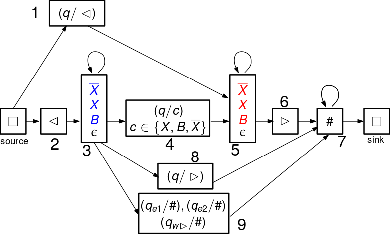
To this end we expand the tile types we have so far, so that the tiles , and come in two different colors: red and blue. Note that there are now six different tiles corresponding to , and : .
We can now partition the ordered pairs of Layer tile types into illegal and legal pairs. If two tiles are an illegal pair for Layer and those two tiles are adjacent in the horizontal direction in a tiling, then that pair of tiles will contribute to the overall cost of the tiling. The set of legal pairs is best illustrated as a directed graph as show in Figure 5.
Definition 7
Legal pairs The pair is a legal pair if one of the following two conditions hold:
- 1.
There is an edge such that is in ’s set and is in ’s set.
- 2.
There is a vertex such that and are edges, is in ’s set, is in ’s set and is in ’s set.
All other pairs of tiles are illegal.
The option is included only to reduce the number of edges in the graph. Suppose instead we added an edge whenever there is a vertex that contains such that and are also edges. Then the ’s could be removed from the graph and the resulting graph would define the same set of legal pairs.
Definition 8
A row of tiles is said to be valid if no two adjacent tiles are an illegal pair. Otherwise the row is invalid.
The set of valid rows corresponds to TM configurations that are a superset of the configurations that the TM would reach in any fault-free33 3 i.e. all rules are obeyed, zero cost computation. We will prove below that each valid row corresponds to a unique Turing Machine configuration to which a rule can be applied. Thus, if a row is valid, then there is exactly one way to tile the next highest row without any illegal computation squares so that the resulting row is also valid.
Since every row must begin and end with a tile and contains no other tiles, a row of tiles is valid if and only if it can be generated by the following process: Follow any path in the graph from the source to the sink. As each vertex is reached, select any tile type from the current vertex and place a tile of the type next in the row. denotes the option of not selecting a tile for the current vertex.
Augmenting tiling rules with colors
The definition of legal/illegal computation squares must be augmented to address the fact that now , and tiles come in two different colors. In a head square, a tile to the left of a head tile must be blue and a tile to the right of a head tile must be red. For example, consider the following computation legal square below:
The in the upper-right corner must be red and the in the lower-left corner must be blue in order for the square to be a legal computation square.
It will als be important to enforce that the only way for a tile to change color from one row to another will be in the presence of the head. so any square of the form
| * | |
| * |
| * | |
| * |
| * | |
| * |
where the two vertically aligned , ’s or ’s have different colors will be an illegal computation square.
To summarize, a square pattern of four Layer tile types is a legal computation square if the square is legal according to the rules translating a Turing Machine to legal and illegal computation squares outlined in Section 2.2 and:
- •
if the square is a head square, then any tile the left of a head tile is blue and any tile the left of a head tile is red
- •
if a tile is directly above a tile , then and have the same color.
Otherwise, the square is an illegal computation square.
Properties of Valid Rows
The graphical representation of valid rows given in Figure 5 makes it clear that local constraints can be used to enforce that a row is valid. In particular, any row that is not valid must contain at least one illegal pair. However, the lemma below is a more useful description of valid rows which will allow us to establish that a valid row corresponds to a configuration of the Turing Machine to which one of the transition rules can be applied. It will be convenient to refer to the tape contents of a row of tiles. This is the row that would result from replacing every tile of the form with .
Lemma 3.1
A row is valid if and only if the row has the following properties:
- 1.
The tape contents of the row has the form:
- 2.
Exactly one tile is a head tile.
- 3.
Any tiles to the left of the head tile are blue. Any tiles to the right of the head tile are red.
- 4.
If there is a or tile, then the state is not in and the head is pointing to one of the tiles from the to the (inclusive).
- 5.
If there is no or tile, then the head is pointing to the leftmost tile and is in state , or .
Proof: We first establish that any valid row must have the five properties outlined in the lemma, starting with property . If a row is valid, then it corresponds to a path from the source to the sink in the graph in Figure 5. Note that every path from the source to the sink must first go through vertex or , so the tape contents of the first tile must be . There is no path back to vertices or , so the first tile is the only tile. If there is a or tile, then the path must pass through vertices or . There is no path back to vertices or , so or only appear once. The only vertices that can come after vertices or is vertex , so only tiles can appear after a or tile. Once vertex is reached, only vertex can be reached before the sink. So after the first , there can only be tiles until the final tile at the sink.
The head tiles are all contained in vertices , , , or . To establish property , note that every path from the source to the sink passes through one of the vertices , , , or exactly once.
If vertex is reached, it occurs before vertices , , , or in the path. Therefore only blue tiles can be to the left of the head tile. If vertex is reached, it occurs after vertices , , , or in the path. Therefore only red tiles can be to the right of the head tile.
If there is no , then the path must pass through vertex . The state must be , , or , and the head points to the leftmost . If there is a symbol, then the path passes through vertices , , or , in which case the state is not , , or and the head points to one of the symbols from the to the .
For the converse, the location of the head determines which vertex from , , , or the path goes through. Any row in which the head points to the symbol that also satisfies all five properties from the lemma can be generated by a path: . Any row in which the head points to the symbol that also satisfies all five properties from the lemma can be generated by a path: . Any row in which the head points to a symbol that also satisfies all five properties from the lemma can be generated by a path: . Finally any row in which the head points to a symbol that also satisfies all five properties from the lemma can be generated by a path: .
Lemma 3.2
If is a valid row, then there is exactly one row that can be placed above such that there are no illegal computation squares that span the two rows and . Row is valid. Moreover, row corresponds to a Turing Machine configuration and represents the configuration resulting from executing one step in configuration .
Proof: Consider a valid row . We will first argue that if there is a row such that if is placed directly above , there are no illegal computation squares, then must be unique.
Since is valid, by Lemma 3.1, it has exactly one head tile. Since each state in the Turing Machine is reached from a well defined direction, a head tile in row must come from a specific location in . Moreover, each head tile in moves to a well-defined location in . This defines a one-to-one correspondence between head tiles in row and head tiles in row . For example, if is a head tile in and the state is reached from the left, then there must be a head tile in row one location to the left such that . Since there is a matching between head tiles in row and head tiles in row and there is exactly one head tile in row , then there is exactly one head tile in row .
Since there are no rules in the Layer Turing Machine in which the head stays in the same location, there will be exactly one head square spanning rows and with a head tile in one of the bottom two tiles and a head tile in one of the top two tiles. The square will have one of the following two forms, depending on whether the corresponding rule moves the head right or left:
| b | |
| y |
| b | |
| y |
Note that the contents of the top two tiles are completely determined by the contents of the lower two tiles and the output of the transition function on input . If either or are a tiles, then their color is also determined by the rules for legal/illegal computation squares and the fact that the head square is a legal computation square.
All other locations in the row have a tape tile in both and . If two vertically aligned tape tiles do not have the same tape symbol and color, then they must be contained in an illegal computation square. If tile in the head square is a tile and is to the left of the head then must be blue. If tile is a tile and is to the right of the head then must be red. Therefore if and are both valid and there are no illegal computation squares spanning rows and , then the contents of are completely determined.
Next we need to show that if is valid, then there is a valid such that there are no illegal computation squares spanning rows and Since is valid, there is exactly one head tile in and therefore corresponds uniquely to a configuration of the Turing Machine. If the head is pointing to a tile in row , then the state is , or . If the head is pointing to a non- tile in row , then the state is not , or . Therefore row corresponds to a configuration of the Turing Machine and there is a transition rule from Figure 3 that applies to this configuration. Let be the row resulting from applying one step of the Turing Machine to the configuration represented by row . Color all the tiles to the left of the head tile blue and all the tiles to the right of the head tile red.
We will first establish that there are no illegal squares spanning rows and . The head square must be legal because it represents one correctly executed step of the Turing Machine. All other tiles outside of the head square are tape tiles and are the same in and because they did not change in the computation step. Moreover since is valid, all tiles to the left of the head square are blue and all tiles to the right of the head square are red. Therefore any tiles outside of the head square have the same color in and .
The final step is argue that the resulting row is valid. Property is satisfied by construction. Row also satisfies Property because it corresponds to a valid Turing Machine configuration and therefore only has one head tile. It remains to establish that satisfies properties , , and . According to the Turing Machine rules (shown in Figure 3) if the head is pointing to a symbol, it will write a symbol and move right into state or , where . The tape contents remain the same and the head is still in between the and symbols. If the head is pointing to a symbol, it writes a symbol and moves left or right. The new state will not be , , or . The tape contents still have the form and the head is still in between the and symbols. If the head is pointing to the or the leftmost , the Turing Machine will either write and move left into a state that is not in or the Turing Machine will write a symbol symbol and move right into state , , or . In the former case, the tape contents will be of the form and the head is in between the and symbols. In the latter case, the tape contents will be of the form and the head will point to the leftmost symbol.
4 Analysis of Layer : Proving Fault Tolerance
The goal of the analysis of Layer is to show that as long as the number of faults is not too large () then the end result will approximate the result of a fault free computation reasonably well.
Section 4.1 associates each illegal pair or square with a particular row and bounds how much a tiling can change from one row to the next as a function of the number illegal configurations associated with that row. Then in order to show that the computation encoded in the tiling makes progress, even in the presence of faults, we define a notion of a complete segment which corresponds to a sequence of rows that represent a complete and fault-free iteration of the Outer Loop of the Layer Turing Machine. In a complete segment, each interval increases in size by and a new interval of length is added to the right end of the non-blank tape symbols. The main goal of Subsection 4.4 is to prove Lemma 4.10 which says that the number of complete segments in Layer is at least , where is the number of faults and the number of intervals in the last row of a fault-free tiling.
In general, the number of steps in an iteration of the Outer Loop will depend on the number of intervals as well as the total length of all the intervals. Thus, it’s possible for faults to create spurious intervals which can cause an iteration of the Outer Loop to take more steps. We define the weight of a row to be the number of intervals and the length of a row to be the number of non-blank tiles, corresponding to non-blank symbols on the Turing Machine tape. In order to lower bound the number of complete segments, we need to bound the effect of faults on the weight and length of a row and prove that they do not slow down the computation by too much. These bounds are given in Section 4.2.
The analysis on the number of complete segments is made more precise in Section 4.4 where we define the function which takes as input a sequence of positive integers and outputs the exact number of steps in one iteration of the Outer Loop if the sequence of interval sizes (from left to right) at the beginning of the iteration is . Section 4.4 gives upper bounds on how much the function can change in a sequence of correct steps as well as how much can change as a result of faults. While the function can be used to bound the number of rows in a complete segment, it is also important to bound the number of rows outside of complete segments. For example a fault could cause the computation to pop into the middle of an iteration of the Outer Loop by having the head move to a completely arbitrary location. Alternatively, a sequence of correct steps could end in a fault before the end of the iteration of the Outer Loop is reached. These bounds are put together to prove Lemma 4.10 which says that the number of complete segments in Layer is at least .
While each complete segment (i.e. iteration of the Outer Loop) results in the creation of a new interval, it is also necessary to argue that the collection of sizes of the the intervals roughly corresponds to that in a correct faulty-free tiling. To that end, we introduce a means of identifying and tracking the intervals as they grow in size and move to the right. Section 4.6 also defines the notion of clean and corrupt intervals. Intuitively, clean intervals are those that have not been affected by a fault lower down in the tiling. The clean intervals are given a unique tag which they keep for the duration of the computation. The analysis only provides a guarantee for the collection of interval sizes for the clean intervals. The lower bound on the number of complete segments proven in Section 4.4 is used to prove a lower bound on the number of clean intervals in Section 4.6. Suppose that the sizes of the clean intervals, from left to right, in the last row of Layer is . Lemma 4.17 states that , the number of clean intervals, in any tiling for Layer is at least .
Section 4.7 defines a potential function which captures how much the sequence differs from the idealized sequence . Lemma 4.22 shows that the value of the potential function is at most . The final lemma required for analyzing the rest of the constructions is Lemma 4.23 which combines Lemmas 4.17 and 4.22 and says that if the sequence of clean intervals at the end of Layer is , then the number of integers in the range that do not appear as an entry in is bounded by .
Layer of the construction for Parity Weighted Tiling and Function Weighted Tiling uses a Turing Machine that sweeps across all of the non-blank symbols. In order to establish that this Turing Machine completes its work in steps, we need an upper bound on the length of a row as a function of and the number of faults in Layer . This analysis is given in Section 4.5. Note that this section is not used in the proof of Gapped Weighted Tiling. We present these bounds just after Section 4.4 because they use the definition for the function which is developed there.
Finally, in order to compare a tiling with faults to an fault-free tiling, we will eventually need to characterize the sequence of interval sizes in an fault-free tiling. This characterization is given in Section 4.8.
4.1 The Cost of a Row
To begin the analysis, it will be convenient to associate each illegal square or pair to a particular row in the tiling. This will be important for accounting for the discrepancy between a faulty tiling and a fault-free tiling with specific occurrences of illegal pairs or squares. The number of such illegal configurations attributed to a row is the cost of a row. Note that when analyzing the overall construction, we will refer to the number of illegal pairs and squares in Layer by . In this subsection, which focuses on Layer , we will drop the subscript and use to denote the number of illegal pairs and squares in Layer .
Definition 9
[Cost of a Row] Fix a tiling of the grid. The rows of the grid will be numbered from bottom to top . Let denote the number of illegal pairs in row . (Note that since is assumed to consist only of tiles, .) If , then is defined to be the number of illegal computation squares contained in rows and . is defined to be the number of illegal initialization squares (which are by definition contained in rows and ). We denote by the total cost of Layer of the tiling, namely the total number of illegal pairs and squares, or the sum of the costs of all rows: .
The following claim which is used throughout the analysis shows that the number of illegal pairs or squares attributed to a row can be used to bound the number of locations where the row differs from the row above it.
Claim 4.1
[Upper Bound on the Distance Between Consecutive Rows] If is an invalid row, then , where is the number of locations where and differ.
Proof: Suppose that row is an invalid row (i.e. ). Let be the number of legal head squares that span rows and . The number of differences between and inside the legal head squares is at most .
Now consider a pair of vertically aligned tiles, and , outside of any legal head square such that . The two tiles must satisfy at least one of the conditions in Facts 2.1 and 2.2 and are therefore contained in at least one illegal computation square. Since each illegal computation square contains two pairs of vertically aligned tiles, the number of differences between and outside of legal head squares is at most .
. We have that the number of head tiles in the row is at least (since two legal head squares cannot overlap, and each head squares contains a head tile in its bottom row). There is no path in the graph shown in Figure 5 from a vertex with a head tile back to another vertex with a head tile. So . Furthermore, since is not a valid row, . The two bounds on together imply that . Therefore .
4.2 Intervals and their Properties
We would like to argue roughly that in any tiling that does not contain a large number of faults, the intervals are organized ”more or less” like in the correct computation. To be able to make this kind of statement precise, we will need to expand the definition for intervals in a row so that intervals are well defined during all points in a valid computation as well as for invalid rows.
We start by defining a weight function on tape symbols, TM states, and tile types.
Definition 10
[Weights of Tape Symbols and TM States] If is a tape symbol, then the weight of , denoted , equals if or , and is otherwise. If is a TM state, then if and otherwise.
Note that the weight states are all states that write a weight- tile, so they encode the presence of a weight- tile in the state. These definitions allow us to assign weights to the tile types.
Definition 11
[Tile Weights] If is a tape tile corresponding to tape symbol , then . If is a head tile corresponding to , then . If a tile has weight greater than , it is referred to as a heavy tile. Otherwise, the tile is called a -weight tile.
We can now formally describe the intervals in a way that is well-defined for an arbitrary row, in particular, the definition is precise, even for a row that represents a Turing Machine configuration in the middle of an execution of the Outer Loop.
Definition 12
[Intervals and their Sizes] An interval is a sequence of more than one tiles in a row, that begin and end with heavy tiles and otherwise contain only -weight tiles. A single tile whose weight is is an interval as well. If is an interval, then denotes the size of , which is the number of tiles in .
For example, the sequence of two tiles is an interval of size and the single tile is an interval of size . The tile would also be the right end of the interval extending to the left and the left end of the interval extending to the right. Therefore, a single tile can potentially be contained in three different intervals. In any row, the sequence of tiles from the leftmost to the rightmost heavy tile define a sequence of intervals. Consecutive intervals overlap by one tile. See Figure 6 for an example.

The length of row is the number of tiles that are not or and is denoted by . The weight of a row of tiles is the sum of the weights of the tiles in that row and is denoted bey .
Fact 4.2
The number of intervals in a row is .
Proof: We prove by induction that the number of intervals contained in the row up to the heavy tile is the weight of the tiles up to and including that tile, minus . This is true for the first heavy tile, and assuming it is true up to the tile, the next heavy tile adds one interval if its weight is , and adds two intervals if its weight is .
The next two lemmas upper bound how much the length and the width of the rows change. The first lemma upper bounds the change over a sequence of rows that do not contain illegal pairs or squares, corresponding to correct Turing Machine steps. The second lemma bounds the change from one row to the next in the presence of faults.
Lemma 4.3
[Change in Length and Weight over Correct Computation Steps] Consider a sequence of rows from to such that the sequence of rows does not contain any illegal pairs or illegal squares. If rows through are not end rows, then and . If is an end row, then .
Proof: The only Turing Machine rule that increases the weight of the configuration is the rule which leads to an end row. Therefore all the rows through have the same weight and .
Each iteration of the inner loop (from an configuration to an configuration where ) increases the size of one interval by one. So each iteration of the inner loop increases the total length by . There are at most iterations of the inner loop. Then the last step also increase the length by . If is in state then there can be an additional increase of one for the symbol that is inserted. Thus the length will increase by at most and . If is an end configuration, the state is and there is not the additional increase to the length and .
Claim 4.4
[Change in Length and Weight in the Presence of Faults] Consider two consecutive rows and in a tiling. Then
Moreover, if is a valid row, then . If is a valid row that is not an end row, then .
Proof: We first account for any increase to the width and length from to that occurs inside legal head squares. Consider each legal head square in rows and . Suppose there are such squares. Each of these squares contains a head tile in the lower level. Also, the total increase in length or weight from to inside these squares is at most since a valid step of the computation will cause the length or weight to increase by at most . There is no path in the graph shown in Figure 5 from a vertex with a head tile to another vertex with a head tile. So . Therefore the total increase in length or weight inside these legal head squares is at most .
If is valid, then there is only one head tile in and therefore at most one legal head square. The only TM step that increases the weight is . If is not an end row (i.e. a valid row that contains ), then the weight does not increase in this square.
Now we will show that any increase to the length or weight from to that occurs outside the legal head squares will be at most . Each illegal square will be given two tokens that can be used to compensate for any increase to the width or length that occurs inside that square. Consider a tile on top of tile . If any of the conditions from Fact 2.1 apply, then both squares that include and are illegal. The width and length can increase by at most . The increase is paid for by a token from each of the two illegal squares that contain and .
If any of the cases from Fact 2.2 apply to and , the weight and length can increase by at most . According to Fact 2.2, and are in a legal head square or an illegal square. In the latter case, the increase in weight is accounted for by a token from the illegal square that contains and .
The only case not covered by Facts 2.1 and 2.2 is when and are both tape tiles and , in which case the length and weight does not increase in that location. This covers the general upper bounds that apply regardless of whether is valid as well as the upper bound on the increase in weight when is valid.
Finally, to bound the increase in length for the special case where is valid, we use again the fact that has exactly one head tile. Suppose that tile is in location . The total increase in length from to at location is at most . Any other increase in length is due to a tape tile in row on top of a tile in row . If there are no such occurrences, then . If there is at least one such vertically aligned pair, then each one can increase the length by at most . Also, by Fact 2.1, each such vertical pair participates in two illegal squares, one to the left and one to the right. Although these squares can overlap, the number of illegal squares is at least the number of such vertical pairs plus . In other words, the total increase in the lengths due to tiles at locations other than is at most . In this case .
4.3 Segments and Complete Segments
In a complete iteration of the Outer Loop of the Turing Machine, each interval increases in size by and a new interval of size is added. Thus, we want to show a lower bound for the number of fault-free iterations of the Outer Loop represented in the tiling (Lemma 4.10). We partition the rows into segments. The end of a segment is reach whenever a row has non-zero cost or is a valid end row. A segment is said to be complete if the last row in the segment as well as the last row in the previous segment are zero-cost rows. Note that this implies that the last row in the two consecutive segments are end rows. Since there are no illegal computation squares contained in the rows of the segment, the segment corresponds to a sequence of fault-free steps of the Turing Machine from one end configuration to the next, which is a complete iteration of the Outer Loop of the Turing Machine.
Definition 13
[Segments and Complete Segments] We will partition the sequence of rows a tiling in to segments going from bottom to top. The first segment consists of the first two rows and . Each new segment begins at the row above the previous segment and ends at the next row that is either an end row or has . Let be the last row of a segment and be the last row of the previous segment. A segment is complete if .
We can now combine the bounds from the previous sections to upper bound the weight and length of a row as a function of the number of segments and the cumulative cost below row in the tiling.
Lemma 4.5
[Upper Bounds on Length and Weight as a Function of Number of Segments and Number of Faults] Let be a row in segment . Then
where .
Proof: Proof by induction on .
Base Case: . The first segment consists of and . , which is the number of illegal initialization squares. We will number the locations of tiles in from left to right so that tiles through are the tiles between the tiles. Square will be the tiles in locations and in rows and . For any let be the number of such that square is an illegal initialization square.
Each tile in can contribute at most to the length and at most to the weight. Let be the locations in that have a tile that is not , or . For every , square is illegal, so . The total contribution to the weight or length of from tiles that are in locations in is at most . Let be the set of locations with a tile. Square is illegal for every , except , so . Each tile contributes to the weight and length of , so the total contribution to the weight or length from tiles in is at most . If a tile in location is , then either square is illegal or location has a tile. Let be the set of locations with a tile. The total contribution to the weight or length from tiles in is at most . A tile does not contribute to the weight or length of . The total weight or length of is at most
Induction step: We will bound the length and weight of the row at the end of segment . Note that if a row is not the last row in the segment, then it must have zero cost. The sequence of rows from to the end of the segment do not contain any illegal pairs or squares and thus correspond to a set of correctly executed Turing Machine steps applied to valid row. Note that the length and width of the row do not decrease with any step of the Turing Machine applied to a valid row. Therefore, it is enough to bound the length and width of the last row in the segment.
Let be the row at the end of previous segment. We consider three cases:
Case 1: . Then . Rows through do not contain any illegal squares or pairs. Row must be an end row, so by Lemma 4.3,
Case 3: and is not the row right after . Then the intervening rows between and are valid. Let be the row right after . The row is valid and not an end row. Otherwise, the segment would have ended at instead of . By Claim 4.4, . By Lemma 4.3, . Therefore,
By Claim 4.4, and . Let . Since , . The rows through do not contain any illegal pairs and are valid. Therefore Lemma 4.3,
The last inequality follows from the facts that and .
4.4 Lower Bound on the Number of Segments
In a fault-free tiling the number of intervals is equal to the number of complete segments because each iteration of the Outer Loop adds one segment. The goal of this section is to show that faults do not change the number of complete segments in the final row of Layer by too much.
Definition 14
[The function ] Define to be the number of intervals in the last row of Layer in an fault-free tiling of an grid.
The goal in this Section is to prove Lemma 4.10 which says that the number of complete segments in any tiling in Layer is at least , where is the number of faults in the Layer tiling. Note that when is , which is the case we will be interested in for all the problems we consider, we are characterizing the number of complete segments tightly, up to low order terms. In order to achieve this tight characterization, we need to specify the exact number of rows in a complete segment which will depend on the sequence of interval lengths. To this end, we define the following function which characterizes the number of steps in a complete segment that starts with a row . Let be the sizes of all the intervals in row from left to right. Define the function as:
| (1) |
If the first row of a segment is a no-cost row, then the segment consists of one or more valid computation steps ending with either a fault or an end row. Lemma 4.6 provides an upper bound on the number of rows in the segment in this case. The upper bound is the function applied to the start row plus some additional terms in the cases where the segment begins or ends with a row with non-zero cost. The proof is a somewhat tedious case analysis because if the previous segment ended with a fault, the computation represented in the segment could begin at any point in the execution of the Outer Loop and it is necessary to consider each possible starting point separately. For example, the fault could cause the head to appear in any location and in any state that is consistent with the horizontal constraints.
The next three lemmas (Lemmas 4.7 through 4.9) then upper bound the amount by which can increase in a sequence of rows. Lemma 4.8 considers the situation described above where the rows are contained within a segment and first row of the segment is a no-cost row. Lemma 4.8 considers a maximal sequence of rows with non-zero cost. Lemma 4.9 considers the initial sequence of non-zero cost rows.
Finally Lemma 4.10 puts all these bounds together to lower bound the number of complete segments.
Lemma 4.6
[Upper Bound on the Length of a Segment] Consider a sequence of rows from to such that the sequence of rows does not contain any illegal pairs or illegal squares. Suppose that the sizes of the intervals from left to right (both clean and corrupt) in row are . If rows through are not end rows, then
If is an end row, then . If and are both end rows, then .
Proof: We will show that if the Turing Machine starts in a valid configuration, then the Turing Machine will reach an end row within correctly executed steps.
Consider a configuration of the Turing Machine that corresponds to a valid row. The configuration is an configuration if the state of the Turing Machine is and the head is pointing to one of the internal weight- symbols in interval or the weight- symbol at the right end of interval .
We will establish that the Turing Machine will reach an end configuration or an configuration for within a certain number of steps. The head moves right in state until it reaches a or symbol. If it reaches a symbol first, then it transitions to and then pointing to a symbol. This is an end state. The number of steps has been
If the head reaches an symbol first in state , it writes a , and then inserts an by moving all the non symbols over by one. Interval now has a symbol on its left end. The number of steps has been at most . When it reaches the state, it replaces the with a , transitions to and moves left. The head moves left in state until it reaches a symbol. We are guaranteed that the left end of interval has symbol but there could be a that comes earlier. Let be the largest index such that the left end of interval is . When the head reaches the left end of interval , it replaces the with , transitions to and moves right. This has been an additional steps. The cycle from the configuration to the configuration is an iteration of the Inner Loop. The total number of steps has been
The number of steps to get to an end configuration from an configuration is maximized if we start in an configuration and for each , after the Turing Machine leaves the configurations, the next time it reaches state is in interval (an configuration). After reaching an configuration, the Turing Machine is guaranteed to reach an end configuration in steps. The maximum number of steps required to reach an end configuration when starting in any state is:
| (2) | |||||
| (3) |
Next we will argue that as long as the initial configuration of the Turing Machine is valid, it will reach the state or an end configuration within a certain number of steps.
If the initial configuration is in state or , the head moves left until a or symbol is reached. Then the state transitions to and moves right. This will be at most an additional steps. Adding this value to the bound from Expression (3):
| (4) |
If the initial configuration is in state then the current symbol is and the configuration is one step away from an end configuration.
If the initial configuration is in state or , then the Turing Machine writes and moves left into state or . The head then moves left until a or symbol is reached. Then the state transitions to and moves right. This will be at most an additional steps and an configuration has been reached. The same bound from (4) applies.
Finally, suppose that if the Turing Machine is in a state . If the current symbol is , it writes a symbol, and moves right into state . The current configuration is a configuration. In this case, the number of steps is the bound from Expression (3) plus .
If the Turing Machine starts in a state and the current symbol is not , then let be the index of the interval that the head starts in. The Turing Machine will insert a symbol and shift the contents of the tape to the right. When the Turing Machine reaches the state, it writes a , and moves left into state . The number of steps has been at most . Interval has now increased in size by . The bound from (4) applies, except that the size of interval is now instead of . The total number of steps to reach an end row is at most
The term comes from the fact that the size of interval is instead of . Plugging in the expressions and :
The simplification in the last line of the equations above use the fact that . The second line gives the first upper bound for stated in the lemma and the last line gives the second upper bound for .
If the initial configuration is an end row, then the Turing Machine writes and moves left into state until it reaches the symbol. The head then moves right into state , which is an configuration. The number of steps so far is exactly . The state changes all symbols to symbols. The Turing Machine maintains the invariant that when in state or , the symbol will mark the right end point of the last interval that has been increased. Therefore, if an iterations of the inner loop that starts in an configuration, the next iteration will start in an configuration. Therefore the number of remaining steps to reach an end configuration is exactly the bound from (3). The total number of steps is exactly the bound given in (4). If the sequence ends before an end row is reached, then the number of rows is less than the bound given in (4).
The following three lemmas will be used to bound the growth of the function . Lemma 4.7 bounds how much can increase as the result of fault-free steps of the Turing Machine applied to valid configurations. Lemmas 4.8 and 4.9 bound how much illegal pairs or squares can cause to increase.
Lemma 4.7
[Upper Bound on Change in in Fault-Free Steps] Consider a sequence of rows through that do not contain any illegal pairs or squares and such that rows through are not end rows. Then
If is an end row, then .
Proof: Since rows through do not contain any illegal pairs or squares, they correspond to steps applied to the valid configuration represented in row . Moreover, the computation does not reach the end of an iteration of the Outer Loop until possibly the last step. Let be the number of intervals in row . If configuration starts in a state , then some interval may increase by one as the head sweeps right, moving all the symbols over by . After this point, each interval can increase by at most before the end of the Outer Loop is reached. Thus, the summation in (1) can increase by at most . If is an end row, then the summation increases by at most . If is not an end row, then and
The first expression above bounds in the case that is an end row and is not an end row. The second expression bounds in the case that neither nor are end rows.
If is an end row, then and a new interval of size is added to to the right end, increasing by an additional .
The first expression above bounds in the case that and are both end rows. The second expression bounds in the case that is not an end row, but is an end row.
Lemma 4.8
[Upper Bound on Change in in a Sequence of Rows with Non-Zero Cost] Consider a no-cost row such that row has a positive cost. Let be the next highest no-cost row after . Let be the number of illegal pairs or squares contained in the rows through . Let be the total number of illegal pairs or squares in Layer . If row is in the segment, then
Proof: By Claim 4.1, . We will let denote . Note that must be a valid row because the row before it, is a no-cost row. Let be the sizes of the intervals in . We start by re-expressing the summation in the definition of from (1):
We will account for how the summation in (1) changes from to . In the worst case, all of the heavy tiles in row are unchanged in and all the locations where the two rows differ result in new heavy tiles in row .
Since and are both valid rows, they have exactly one tile which is the right end of the right-most interval. The sum is exactly the distance from the left end of interval to the tile. The position of the tile is at most spaces to the right in than it is in , so the value of the summation in (1) increases from to by at most as a result of the existing heavy tiles in . There are at most new heavy tiles in that were not in , each of which can create at most two new intervals (since the weight of every tile is at most ). Each new interval can increase the sum by at most which is at most . The increase due to the new intervals is therefore at most . Therefore .
Since has non-zero cost, it is the last row in some segment , where . The number of intervals in row is , which according to Lemma 4.5, is at most . Using the same lemma, we can bound by which is at most since . Plugging the bounds in, and using the fact that , we get
Lemma 4.9
[Upper Bound on Change in the Initial Sequence of Rows with Non-Zero Cost] Let be the smallest index such that is a no-cost row. Let be the number of illegal pairs and squares contained in rows through . Then .
Proof: By Lemma 4.5, the weight and length of is at most , where is the number of illegal initialization squares. By Claim 4.4, the weight and length can increase from to by at most , where is the sum of the costs of rows through . because the first rows all have non-zero cost. Also . Therefore the weight and length of is at most
The summation in the definition of is maximized if the contents of the row consists of heavy tiles, in which case there are intervals all of size . Then is which is at most . The additional cost of is incurred only if is not an end row, in which case . Therefore
Lemma 4.10
[Lower Bound on the Number of Complete Segments] Let be the number of illegal squares or pairs in Layer of a tiling of the grid. Then the number of complete segments in Layer is at least .
Proof: The main work of the proof is to show that the number of segments (complete or not) in Layer is at least . Each segment ends on a row that incurs a cost or ends on an end row, corresponding to the last row of an iteration of the Outer Loop. Each illegal square or pair can cause the end of at most one segment. Therefore, if there are at least segments, then there must be at least segments that end with a zero cost row and such that the segment before also ends on a zero cost row. These are, be definition, complete segments.
Consider a tiling of the grid that has a total of illegal pairs and squares. Number the segments from bottom up. We will denote the number of row in segment by . Let be the segments in the unique tiling in Layer that has no illegal squares or pairs, which we call the no-cost tiling. There is one interval after the first segment (which just consists of the initial row). Then in a fault-free tiling every segment corresponds to one iteration of the Outer Loop in which exactly one interval is added in the last step. Therefore in a fault-free tiling the number of complete segments is equal to the number of intervals in the last row, which is . We will show that
Thus if is large enough to accommodate segments in an fault-free tiling, then is large enough to accommodate segments in a tiling with illegal pairs or squares.
A segment will be called big if it has more than one row and otherwise it is called small . In a big segment, all the rows except possibly the last row of the segment have . If a row is valid () and there are no illegal squares contained in the row and the row above it (), then according to Lemma 3.2, the row above is the unique row representing one step of the Turing Machine applied to the configuration corresponding to , which is also a valid row. Therefore, if a segment has more than one row, all the rows in the segment are valid and there are no illegal pairs or squares contained in the rows of the segment.
Finally, we will partition the illegal pairs and squares in Layer according to where they are located with respect to the big segments. If is small, then . Otherwise if is big, let be the largest such that is also big. The quantity is defined to be the number of illegal squares contained in the set of rows from the last row in through the first row in . If is the first big segment then, is the number of illegal pairs and squares contained in the rows from through the first row in , including the illegal initialization squares. Note that .
Note that in any tiling, the first segment consists of rows and , so we will only be concerned with bounding the number of rows in all the segments, except the first segment. We will define a quantity for each segment indexed by . If the segment is small, then . If the segment is big, then , where is the first row in the segment. If the last row of the previous segment is a no-cost row, then it must be an end row. According to Lemma 4.6, is an upper bound on the number of rows in the segment. If the last row of the previous segment has non-zero cost, then and the number of rows of the segment is at most , where is the first row in the segment. Therefore
Using the bounds from Lemma 4.5 and simplifying, and ,
| (5) |
We would like to bound how much the parameter can grow from one big segment to the next. To that end, we define to be the increase in . If is small, then . Otherwise , where is the largest such that is also big. If is the first big segment then, . For any :
The goal then is to bound . Suppose that is a big segment that is not the first big segment. Let be the last big segment before . Let be the first row of , be the last row of and the first row of . . We will bound and separately.
We first bound . There are two cases:
Case 1: has zero cost. Let be the row after . Since is the last row in segment , it must be an end row. Row represents the first configuration in the next iteration of the Outer Loop. Since the intervals do not change in the first step of the Outer Loop, . If is also a no-cost row, then it is the first row in a big segment, which means that is the first row in and . In this case, and . If has positive cost, we can apply Lemma 4.8 with and to get that
Case 2: has positive cost. We can apply Lemma 4.8 with and to get that
We now use Lemma 4.7 to bound . If the row before has zero cost, then it must be an end row, and . If the row before has positive cost, then . Note that if the row before has positive cost, then . Therefore, we can combine the bounds to get:
By Claim 4.4, . Therefore
The bound for comes from adding the bounds for and for , to get
| (6) |
The bound for in 6 applies to the case where is a big segment that is not the first segment in Layer . If is the first big segment, then by Lemma 4.9,
If is not a big segment, then . In either case, using the fact that , one can verify that is bounded by the expression given in 6. Therefore
By replacing or with and replacing with , the second summation can be upper bounded by . The dominant term in the expression above is from the term. Using the fact that and , we can bound
The expression in the max function is maximized for t = 2m/3. Therefore:
Putting this bound together with the bound from (5):
Now we turn to the fault-free tiling. For , in the first row of , there are intervals of sizes . Therefore and . Letting , we want to show that
We will lower bound the difference of the two summations:
4.5 Upper Bound on the Length of a Row
Layer of the construction for Parity Weighted Tiling and Function Weighted Tiling uses a Turing Machine that sweeps across all of the non-blank symbols. In order to establish that this Turing Machine completes its work in steps, we need an upper bound on the length of a row as a function of and the number of faults in Layer . In this section we present the upper bound on the length of a row required for this analysis. Note that this section is not used in the proof of Gapped Weighted Tiling. We present these bounds here because they use the definition for the function which is developed in the previous section.
Lemma 4.11
[Lower Bound on the Change in ] Consider any two consecutive segments which end at rows and , respectively. Then . If and are no-cost rows (meaning the segment ending in row is a complete segment, then .
Proof: In a complete segment, the size of each segment increases by and there is a new segment of size added to the right end. Therefore the sequence becomes . Therefore the value of goes from
The overall increase is . The length of row is equal to , so the value of increase by at least .
Consider a sequence of of rows that do not contain any invalid squares. This sequence of rows represent correctly executed steps of the Turing Machine applied to a valid row. Each iteration of the inner loop causes one of the intervals to increase in size and the other intervals to remain the same which can only increase . The only point at which the value of can decrease is when the head is moving right as it inserts a new blank symbol into an interval. As the rest of the tape symbols are moved to the right, one interval which holds the current location of the head can be temporarily decreased in size by . This can decrease the value of by at most . By the time the head reaches the right end of the tape symbols, the sizes of all the intervals are at least their original size. This can contribute a decrease of at most . If the last row in the previous segment has non-zero cost, There may be tiles that change from one row to the next outside of a valid computation square. The worst case is if a tile of weight changes to a tile of weight . This would cause three consecutive intervals of sizes to be merged into one interval of size . The net effect is that can increase by at most four times the length of row . Therefore, .
Lemma 4.12
[Upper Bound on the Number of Segments] If row is the last row in a tiling in Layer and is the number of illegal pairs or squares in Layer of the tiling, then if , the number of segments in Layer is at most .
Proof: Consider a complete segment. The weight of the row at the end of the segment is exactly one larger than the weight of the last row of the previous segment. At the end of the segment, there have been such increases overall. Furthermore, none of the valid Turing Machine rules decrease the weight of a row, so in any valid computation square the weight of the two top tiles is at least the weight of the two bottom squares. The difference in weight between two vertically aligned tiles is at most two. The number of vertically aligned tiles that are not the same and are outside of valid computation squares is at most . Therefore the weight of any row after the first segments is at least .
Let be the row just before the beginning of a complete segment. Then the value of increases by at least . This means that by the end of the segment, the total increases that occurred during complete segments is at least
In each incomplete segment, the value of can decrease by at most , where and are an upper bounds on the length and weight of a row that has occurred so far. By Lemma 4.5, and . Therefore the total decrease which has occurred so far in all the incomplete segments is at most . Therefore, by the end of the segment, the value of is at least
. For and , then this function is at least .
If a complete segment begins in row , then by Lemma 4.6, the length of the segment is exactly . If the total number of segments is larger than , then the total number of complete segments that happen after the first segments is at least . Each of these segments lasts for at least rows. This contradicts the fact that there are at most rows.
Lemma 4.13
[Upper Bound on the Length of a Row] If row is the last row in a tiling in Layer and is the number of illegal pairs or squares in Layer of the tiling and , then .
4.6 Clean and Corrupt Intervals
In order to track the sizes of the intervals, we will need a somewhat sophisticated definition, which will recursively designate each interval in row clean or corrupt. Intuitively, a clean interval in row is an interval that is unaffected by an illegal pair or square in rows through . Each clean interval in a row is given a tag. The clean intervals within a row all have unique tags. The tags allow us to track the intervals while the intervals shift and grow as the computation progresses (extending upwards in the tiling). Lemma 4.17 then uses the lower bound on the number of complete segments from Section 4.4 (Lemma 4.10) to lower bound the number of clean intervals in the last row of Layer . Tagging the clean intervals will be useful so that we can argue more precisely about how the sizes of those intervals grow.
We are only be able to characterize the sizes of the clean intervals as faults can cause the sizes and number of an intervals to change in unpredictable ways. Consider for example an interval of size and a fault which causes a in the middle of that interval to change to an in the following row. The interval of size splits into two different intervals whose sizes sum to .
To write down the definition of clean and corrupt intervals, we need a notion of a distance between sequences of tiles:
Definition 15
[Row Distance on a Sequence of Locations] The distance between two tiling rows and is the number of locations where and differ and is denoted by . If is a sequence of tile locations in a row of length , and and are two tiling rows, then is the number of location in where and differ.
We will also need the following notation: For any valid row , let denote the unique row that can be placed above with no illegal squares. According to Lemma 3.2, represents the application of one step of the Turing Machine to row .
Consider two consecutive rows in the tiling and . If is valid, then is well-defined and we want to assess whether a clean interval in row remains clean in according to whether it is equal to the corresponding interval in . On the other hand if is not valid, then the row will not necessarily correspond to a valid Turing Machine configuration and there is not a well-defined expectation for what should be. In this case, we just compare to in determining whether each clean interval in remains clean in .
Definition 16
[Clean and Corrupt Intervals and Tags] is assumed to consist of all tiles, so the definition of clean or corrupt starts with . For the intervals in row are designated as clean or corrupt, and the clean intervals will be tagged by positive integer numbers (which can be viewed as ”names” of the clean intervals). This is done recursively, as follows.
First, a comparison row is determined, the intervals in are designated as clean or corrupt, and the clean intervals in are tagged. This is then used to decide about the clean and corrupt intervals of as well as the tags for the clean intervals in . We consider three cases:
- 1.
Case 1: . The comparison row is set to be the correct starting row:
Since this row is correct, we already know the assignment of its clean and corrupt intervals: The only interval in is , which is designated as clean and assigned the tag .
- 2.
Case 2: and is invalid. Then . The intervals in have recursively been designated as clean or corrupt. Moreover, the clean intervals have been assigned tags.
- 3.
Case 3: and is valid. Then . Order the intervals in and from left to right. The interval in is given the same clean/corrupt designation as the interval in . If the interval is clean, then the tag is also the same. Claim 4.14 below shows that since is valid, the number of intervals in is either the same or one larger than that of . If has one more interval than , then the new interval is the rightmost interval. The new interval is designated as clean and given the tag .
We now use the designation of clean or corrupt intervals in to determine which intervals are clean and corrupt in . For each interval in , let be the sequence of tiles in that interval. If , then the interval is corrupt in . If , then the interval adopts the same clean/corrupt designation as in . If the interval is clean then it adopts the same tag as the corresponding interval in .
The following Claim shows that Case 3 of the above definition is indeed well defined.
Claim 4.14
[Change in the Number of Intervals in One TM Step] If is a valid row, then and have the same number of intervals, except if has the form in which case has a new interval. The new interval is the right-most interval in and has size .
Proof: By Fact 4.2, we know that the number of intervals is one less than the weight of the row. The only TM rule that increases the total weight of the tiles (namely, the only legal head square whose weight of top two tiles is bigger than that of its bottom two tiles) is . By inspection of Figure 5, the only valid row which has the tile as its head tile, is of the form . Therefore if any other rule is applied, the number of intervals is the same between the two rows. Note that is a heavy tile so is the right end of the right-most interval in . When the rule is applied, the two tiles in become in . Since and are both heavy tiles, the interval to the left of the does not change and the new interval has size .
In order to use the tags in Definition 16 to track intervals, we need the following lemma about the tags:
Lemma 4.15
[Interval Tags are Unique] Within a row , all the tags of clean intervals are unique and . If a clean interval in has a tag , then there is a clean interval with tag in row .
Proof: By induction on . There is only one possible clean interval in row . If row has that interval, then its tag is .
For the inductive step, suppose that is invalid. Then in Definition 16, . The only way for an interval to be clean in is for that interval to be identical to a clean interval in in which case the interval has the same tag in as it does in . If the intervals all have unique tags in then they also have unique tags in .
If is valid, then . There is a one-to-one correspondence (that preserves tags) between the clean intervals in and the intervals in , except for the fact that might contain an additional new interval with tag . If all the intervals in are unique and , then all the intervals in are unique and . The only way for an interval to be clean in is for that interval to be identical to a clean interval in . If the tag of a clean interval in is , then it corresponds to a clean interval in whose tag is , which in turn corresponds to a clean interval in .
Lemma 4.16
[Upper Bound on the Loss of Clean Intervals] The number of tags such that there is a clean interval with tag in but there is no clean interval with tag in is at most .
Proof: By Lemma 3.2, if , then is the same as , which means that represents a correctly executed step of the Turing Machine on the configuration represented in the valid row , and row is also valid. Thus no clean intervals are lost from to , although it’s possible that a clean interval with tag is added in row .
If , then row is not valid. By Definition 16, is compared to in determining which intervals in are clean. Each clean interval in that is unchanged in remains clean in . Therefore if a clean interval with tag that is present in does not appear in , there must be a tile in the interval where and differ. Each tile in is included in at most intervals, so the number of intervals that are clean in that are no longer clean intervals in is at most , which by Claim 4.1 is at most .
Now suppose that is valid () but . is compared to in determining which intervals are clean or corrupt. Every clean interval in corresponds to a clean interval in with the same tag. Every clean interval in that fails to appear in must contain a location where and differ. Since each tile participates in at most intervals in , the number of clean intervals in that are no longer clean intervals in is at most . We will now argue that .
and only differ in two locations. The other locations are all tape tiles. If one of these tape tiles in is not the same in , then those two vertically aligned tiles are in an illegal computation square. Now consider the legal head square resulting from putting on top of . If either tile in the top row of this square differs from the two corresponding tiles in then the head square is illegal. Therefore in each location where and differ, the two vertically aligned tiles in and in that location are contained in an illegal computation square. Since each illegal computation square contains at most two pairs of vertically aligned tiles, the number of locations where and differ is at most .
Lemma 4.17
[Lower Bound on the Number of Clean Intervals] Let be the number of illegal squares or pairs in Layer of a tiling of the grid. Then the number of clean intervals in the last row of Layer is at least .
Proof: By Lemma 4.10, the number of complete segments in Layer is at least . Since each complete segment corresponds to an fault-free iteration of the Outer Loop and since one new clean interval is added in each iteration of the Outer Loop, the number of clean intervals that are created in Layer is at least . Each of these clean intervals is tagged with the row number in which it first appears, which is the last row in that segment. Therefore, each of the clean intervals created has a unique tag. By Lemma 4.16, the number of tags such there is a clean interval in some row but no clean interval with tag in row is at most . Therefore the number of clean intervals in the last row of Layer is at least .
4.7 The Potential Function
In addition to giving a lower bound on the number of clean intervals in a tiling, we will want to show that the sizes of those intervals do not deviate too much from the sizes of the intervals in a tiling with no illegal pairs or squares. In an fault-free computation, if the number of intervals at the end of an iteration of the Outer Loop is , then the sizes of those intervals from left to right will be . The function captures the extent to which the interval sizes differ from this ideal case.
Definition 17
Consider a sequence of positive integers .
Note that . It will also be convenient to refer to the value of for a row in Layer of a tiling. If the sizes of the intervals in row (from left to right) is , then . If does not have any clean intervals, then is defined to be .
The primary goal of the analysis in this section is to prove Lemma 4.22, which says that if is the last row of Layer in a tiling, and is the number of illegal pairs or squares in Later , then is bounded by .
4.7.1 Features of the function
The analysis of each layer will bound the value of by a constant times the number of illegal pairs and squares. At various points in the analysis, we will need to deduce features about the sequence of sizes of the clean intervals based on the bound for the value on the value of . The following three technical lemmas describe the required features and argue that they follow from the bound on .
Lemma 4.18
Consider a sequence such that each . Let denote the set of integers occurring in the sequence with repetitions removed. Then
Proof: The value of is minimized if the ’s are sorted in decreasing order, so we will assume this is the case. Let be the set of integers in the range from through . Define and . If the sequence is sorted in decreasing order then value of is equal to . Furthermore . If , then
If , then
Lemma 4.19
Consider a sequence whose value is at most . Then at least of the ’s are at least at least .
Proof: We will prove that if there less than of the ’s are at least at least , then the value of is strictly larger than . The value of is minimized when the sequence is sorted in non-increasing order, so we will also assume that the ’s are sorted accordingly.
If there are less than of the ’s in the sequence that are at least at least , then there are more than of the ’s that fall in the range from to . This implies that there are more than of the ’s such that . Each such value contributes at least to the sum defining . Since all the terms in are non-negative, the lemma follows.
Lemma 4.20
Consider a sequence . If and is removed from the sequence then the value of for the sequence decreases. If any is removed from the sequence, the value of increase by at most .
Proof: If then the first term in the sum defining is . Since is positive, the value of increases when is removed. If , the last two terms in the sum defining are . If is removed, these two terms are placed by , which for positive is less than .
Finally, we consider the case that is neither, nor . When is removed, the two terms are replaced by . If , then the original expression is which is replaced by and the sum decreases.
If , then . Meanwhile the new expression is maximized when in which case . We have that
4.7.2 Bound on the value of in a tiling
The analysis for Layer must bound the value of in the last row of Layer as a function of the number of illegal squares and pairs in Layer . We start by analyzing a sequence of rows with no illegal pairs. Lemma 4.21 gives an upper bound on the amount by which can increase over a sequence of fault-free steps (corresponding to no-cost rows). Then Lemma 4.22 gives an upper bound on as a function of the number of faults in all the rows below in the tiling.
Lemma 4.21
[Upper Bound on the Increase in A Over a Sequence of No-Cost Rows] Consider a sequence of consecutive rows in a tiling of the grid, beginning with row and ending on row . Suppose that the tiling from through does not contain any illegal pairs or squares. Then . If is an end row then .
Proof: Each row proceeding upwards from corresponds to one step in the computation of the Turing machine. All the intervals (clean and corrupt) will be numbered from left to right, and we will track the changes to the interval sizes by functions. So a would indicate that the interval as increased in size by . Note that a change to interval will only affect the value of if is a clean interval. We will use to denote the number of clean intervals and to denote the total number of intervals. Note that the number of intervals does not change in one iteration of the Outer Loop, except in the last step.
At the start of an iteration of the Inner Loop, the state is . We will call a row an row, if the state is and the head is in interval . Since the intervals overlap, the head could possibly be in two intervals at the same time, such as . In this case, we say that the head is in the interval to the left. In analyzing the sizes of the intervals, it doesn’t matter where in interval that the head begins. When the TM is in state , the head moves to the right past any symbols until it reaches an or a tile at which point it changes state. Thus, in any consecutive sequence of rows in which the state is , the head remains in the same interval and the interval sizes do not change.
We will consider different subsequences of rows corresponding to different portions of an iteration of the Outer Loop.
- 1.
The subsequence starts with an row and ends with an row. After the iterations of the inner loop, the intervals through will have increased in size by and all other interval sizes will stay the same: .
- 2.
The subsequence starts with an row and ends before an row is reached. If the head never reaches the right end of interval , the intervals do not change. If the head sweeps past the right end of interval , then the size of interval increases by . (.) If the sequence ends while the head is in interval before reaching the tile, then the left end of interval has been moved over but the right end has not been moved over. The effect is that interval has decreased in size by : . If the subsequence ends after the head has reached the tile, the state will be or . In this case, all the tiles have been moved over and there is no change.
- 3.
The subsequence starts in a row that is not an IS row and ends when the first is reached. If the initial state in the subsequence is or , then the head just moves left until it reaches a or symbol, at which point the state transitions to . The intervals do not change. If the head is in the middle of sweeping right, then the state is , or . Suppose that the head starts in interval . The size of interval is increased as the head sweeps right. When the head has finished sweeping to the right, all the tiles have been moved over and the net effect is .
- 4.
The subsequence starts in the state and stops on or before . The head sweeps left until reaching . The intervals do not change, so all ’s are .
- 5.
The subsequence starts in an row and ends on or before the next end row. The head moves right until it reaches the symbol. The tile become which means that . Then become which means a new interval of size has been added. The last step in which changes to does not change any of the intervals.
Let be the indices of the clean intervals in . Let denote the size of interval . The value of is:
We first consider the case in which is a end row. If the sequence ends before the first Inner Loop begins, the net effect on is because none of the intervals change in size. Otherwise, the sequence can then go on to complete iterations of the inner loop which causes the first intervals to increase in size by . If is the number of clean intervals among the first intervals, then , which can increase by at most because only the term changes and that term can only change by . If the sequence goes on to an incomplete iteration of the Inner Loop, the next clean interval could have increased ( and the change to is still at most . It’s also possible that the sequence ends while the head is sweeping right, in which case for some clean interval . This can increase by an additional for a total increase of . If the sequence completes all the Inner Loops, then all the clean intervals will have increased in size. In this case, none of the terms inside the sum in the expression for change. However the last term will increase by . Finally, if the sequence completes the entire Outer Loop, an additional interval of size is added to the end, so there is a new . The net effect on from the beginning of the sequence is .
Thus if is a end row, and the sequence ends before the next end row, can increase by at most . Moreover if the sequence is one complete iteration of the outer loop (i.e. if and are end rows), then .
Now suppose that the sequence begins in an arbitrary location in the middle of the middle of the Outer Loop. The worst case, is that the sequence starts during a right sweep in an inner loop. There is possibly a if the head starts out in a clean interval which is increased as the head sweeps right. ( can increase by at most .) Then after a one or more complete iterations of the Inner Loop, a consecutive sequence of clean intervals could have increased in size by . ( can increase again by at most .) Then the sequence can end in the middle of an iteration of the inner loop in which case, there could also be a for the interval where the head ends up. (Another increase to of at most .) The total increase to is bounded by . Thus, if the sequence does not contain any end rows (i.e. the sequence is contained within one iteration of the Outer Loop), then the increase to is at most .
If the sequence begins at an arbitrary location in the middle of the Outer Loop and completes the Outer Loop (i.e. ends on an end row), then there could be a if the head starts out in a clean interval which will be increased as the head sweeps right. ( can increase by at most .) In addition, the next iterations of the Inner Loop will start with some interval and increase all the intervals to the right of , this will result in and finally, a new clean interval of size will be added to the right end. These changed can increase by at most because only the term increases by . The effect of increasing the last clean interval by and adding a new interval of size cancels out as argued above. Thus if the sequence starts in the middle of an Outer Loop and runs to the end of the Outer Loop, increases by at most .
We have argued that if the sequence from through does not contain any end rows (i.e. the sequence is contained within one iteration of the Outer Loop), then the increase to is at most . If sequence does contain an end row, let be the first end row and be the last end row of the sequence. Since going from end row to end row, does not change the value of , . A sequence that is contained in an Outer Loop and ends on a end row increases by at most , so . A sequence that is contained in an Outer Loop and begins with an end row increases by at most , so . Putting the inequalities together gives that .
Lemma 4.22
For any ,
Proof: By induction on . Base case: . The only possible clean interval in row is . If has this clean interval, then . If does not have any clean intervals, then by definition.
Inductive step: Suppose the intervals in are determined by comparison to row . Every clean interval in corresponds to a clean interval in . The only way can change from to is if a clean interval is removed. Each location where and differ can remove at most three clean intervals from to row . Each removed clean interval can increase by at most . If , , and are the sizes of three consecutive clean intervals in and the interval of size is not present in then:
Therefore .
Case 2: is valid and there is an illegal square in rows and . Since is valid, . If we were to put row on top of row , the two rows would not contain any illegal pairs or squares and would therefore satisfy the conditions of Lemma 4.21. So .
Every location where and differ must be contained in at least one illegal square and a square contains two locations.To see why this is true, consider placing over . The two rows do not contain any illegal pairs or squares. Since is valid, there is exactly one head square that contains the head tile in the two rows. If differs from at eiher of those two locations, then the square must be illegal. In all other locations, and contain the same tape tile. If differs from the in any of those locations, then that would correspond to two vertically aligned tape tiles that are not the same. Any such vertically aligned pair is contained in two illegal squares.
Therefore
Putting the two inequalities together and using the fact that , we get that
Case 3: Rows through do not have any illegal pairs or squares. Then is an end row. By Lemma 4.21, . Since , then .
Case 4: and there is a such that . Let be the largest such that and .
The rows through do not contain any illegal pairs or squares. By Lemma 4.21, .
By the inductive hypothesis,
Therefore, using the fact that and , we have that
We can put Lemmas 4.17 and 4.22 together to get the following Lemma which summarizes what is needed from the analysis of Layer for the next Layer. In particular Lemma 4.23 bounds the number of interval sizes in the range through not represented in the last row of Layer .
Lemma 4.23
[Bound on the Number of Missing Interval Sizes] Consider a tiling of the grid. Let be the tiling in the last row of Layer . Let denote the set of integers such that if there is a clean interval of size in row . Let denote the total number of faults in Layer . Then
Proof: Let denote the sizes of the clean intervals, from left to right, in row . We can remove all the intervals of size and according to Lemma 4.20, the value of for that sequence will only decrease. Since the size of the remaining intervals is at least , we can apply Lemma 4.18 with ,
By Lemma 4.17, , the number of clean intervals in the last row of Layer is at least , and therefore . Since , by Lemma 4.22, the value of , which is the value of for the last row of Layer is at most .
4.8 Characterizing the intervals in an fault-free tiling
In order to compare a tiling with faults to an fault-free tiling, we will eventually need to characterize the sequence of interval sizes in an fault-free tiling. At the end of every iteration of the outer loop, the sequence of intervals starts at some number and decreases by , going from left to right, until the last interval which has size . In the middle of an iteration of the Outer Loop, the sequence of interval lengths can differ slightly from this ideal case. The extent of the difference is characterized in the lemma below.
Lemma 4.24
[The Sequence of Interval Sizes in a Fault-Free Tiling] Consider a row that represents the configuration of the Turing Machine in an fault-free execution in which the TM is in the iteration of the Outer Loop. The number of intervals in is . Define the set such that if and only if there is an interval of size in row .
- 1.
The sizes of the intervals form a non-increasing sequence from left to right.
- 2.
There are at most two intervals with the same size and the largest size only appears once.
- 3.
- 4.
Proof: The Turing Machine starts with one interval of size . After complete iterations of the Outer Loop, intervals have been added, for a total of intervals. The sizes of those intervals is . This sequence satisfies properties through . Now consider the next execution of the Outer Loop. After the complete iterations of the Inner Loop, the leftmost intervals have increased in size by , so the sequence is . This sequence also satisfies through . At this point and .
In the middle of the iteration of the Inner Loop, the intervals stay the same as the head sweeps left. When the head reaches the left end of interval , it sweeps right and increases the size of that interval by when it reaches the right end of the interval. As the head sweeps to the right moving all the tape symbols over by , one of the intervals to the right of interval is decreased temporarily by . So if and is the current sequence, then , except for one where . The sizes are non-increasing from left to right (property ). The only two intervals with the same size are and (property ). All numbers are in the range (property ), and the two numbers in the range which are not in are and (property ).
After iterations of the inner loop, the sequence of interval sizes is . The next iteration of the Outer Loop begins when an interval of size is added to the right end.
Lemma 4.25
[Bounds on ] The function . In addition is and the exact value of can be computed in time that is poly-logarithmic in .
Proof: In an fault-free tiling, the number of intervals increases by whenever an end row is reached. Row is an end row which has one interval. After the end row, there are intervals, of sizes . By Lemma 4.6, the number of rows until the next end row is , where the sizes of the intervals are numbered from left to right. Plugging in , for gives . Thus is the largest value of such that
| (7) |
Let be defined to be
Note that . Therefore there is a constant such that if , them which means that . To get the more precise lower bound on :
If , then , which means that . Finally, since has a closed form that is a degree polynomial in , it is possible to binary search on the range to find the larges value for which the Inequality (7) holds. The number of iterations is and computing the value of can be done in time that is polynomial in .
5 -Gapped Weighted Tiling is NEXP-complete
Containment is straight-forward since given a number expression in binary and a tiling of an grid, which is exponential in , the size of the input the cost of the tiling can be computed in time and it can be verified whether the cost of the tiling is or at least for some constant .
To establish the hardness of the Gapped Weighted Tiling Problem, we will show for and arbitrary , a reduction to a translationally invariant 2D Tiling with an gap. Specifically, we will show a finite set of tiling rules so that, by a polynomial time computable function ,
- •
If , then there is a cost tiling of an grid using the tiling rules.
- •
If , then any tiling of an grid has cost at least .
Since , there is an exponential time verifier that can verify that a string given a witness whose size is exponential in . We will assume that on input , if , then the verifier runs in time and space at most , including the space required for the witness. This can be achieved by padding:
Claim 5.1
[Padding Argument] If , then for any constant , is polynomial-time reducible to such that the verifier for uses time and space .
Proof: Suppose that the verifier for uses time (and space) at most . Define a new language
where . A verifier for will first make sure there are the correct number of ’s at the end of the input, then will erase the ’s (incurring a small overhead). Then will simulate on . The running time is close to . The length of the input is . So as long as , the running time will be .
The large cost for is achieved by independent computations, each of which will run the verifier for on the input . First we need to establish that there are enough intervals created in Layer that are wide enough to simulate the execution of the verifier. Lemma 5.2 shows that the analysis provided in Section 4 is sufficient to establish that there will be at least intervals of size at least .
Lemma 5.2
[Results From Layer ] Consider a tiling of Layer and let be the total number of illegal pairs or squares in the tiling. Then there are at least clean intervals of size at least .
Proof: Let be the sequence of sizes of the clean intervals in a tiling of Layer . Lemma 4.23 says that the number of integers in the range that are not present in the sequence is at most . By Lemma 4.25, , so there are at least numbers in the range of value at least . At most are missing. Therefore the number of clean intervals of size at least is at least .
It now remains to give the description of the constructions for Layers and .
5.1 Layer 2
Since Layer runs bottom to top and Layer runs top to bottom, the only interaction between Layers 1 and 2 takes place in , which is the last row for Layer and the first row for Layer . The translation rules from Layer to Layer will ensure that the heavy tiles from Layer are copied as tiles in Layer . Thus, the intervals in Layer will have an on each end.
The Layer tiling rules also enforce that an tile must go above an tile and can not be placed above any other tile. This implies that in a no-cost tiling, the tiles form columns of ’s in Layer 2. In the vertical strip of tiles between each column of ’s, there will be an independent Turing Machine computation. The tiling rules will enforce that the head of each Turing Machine stays within it’s strip.
The tile types for Layer 2 include , , and . Any square in which is directly above or below a tile that is not or is illegal. Similarly for , any square in which is directly above or below a tile that is not or is illegal. Since the tiles are only around the perimeter of the grid, the ’s and the ’s must form columns in the interior of the grid. An example is shown in Figure 7.

There will also be tile types representing the execution of a Turing Machine in between the two columns of tiles. The tape symbols for the Turing Machine will be and the states will be . Thus, there will be tile types for each of the tape symbols (called tape tiles) and tile types for state-symbol pairs (called head tiles) of the form () where is a state and is a tape symbol.
The relationship between Layer and tiles is summarized below. The rules will enforce the condition that for any tile directly below a tile, if the tile type in Layer is as indicated on the left, then the tile type for Layer must be one of the choices on the right.
The translation rules enforce that the intervals in the last row of Layer are preserved in the first row of Layer , except for intervals of size which correspond to a tile of weight in Layer .
In addition, Figure 8 shows the initialization rules for Layer . The meaning of the graph is that any square with in the top row and two Layer tiles in the bottom row that do not correspond to an edge from to in the graph is illegal. This resolves the ambiguity in whether a weight- tile in Layer gets copied to a , , or a . If an interval has no illegal initialization squares, the interval could be or . These are the only possibilities for intervals of size or . If an interval has has no illegal initialization squares and has size at least , the the interval must have the form .

Figure 9 shows and example of a possible last row for Layer and its correct translation to the first row of Layer .

The Turing Machine that is executed within each strip continually increments a binary counter that is written in reverse on the tape. We call this the Binary Counter Turing Machine. The rules are summarized below.
In a single iteration, the head starts pointing to the in state . It transitions to and moves right. The head then moves right (in state ) changing ’s to ’s until a or is encountered. The or is overwritten with and the head transitions to and moves left until the is reached again. If the head ever reaches the symbol at the right end of the interval, the Turing Machine hits an infinite loop and never changes state again.
The TM rules are translated into legal and illegal squares as described in Section 2.2. The tile is treated as a tape symbol. For example, the rule would mean that the square shown is legal. (Recall that the computation for Layer goes from top to bottom.)
The rule would mean that the square shown is legal.
The tape symbol prevents the head from trying to move left into the on the left and the symbol prevents the head from moving into the on the right. Thus, if the strip is not wide enough for the computation, the head reaches the symbol and the computation eventually gets stuck and does not advance. This does not cause any additional cost, so for every strip in which the computation starts in configuration , there is always a unique way to tile that strip so that it does not contain any illegal squares.
If the goal is to produce a string in the last row of Layer , one could calculate the number such that after steps, the Turing Machine is in state and contents of the counter is . Note that the contents of the counter always ends in , so in order to produce an arbitrary string , one can produce and then ignore the last bit. The lemma below implies that the function mapping to is polynomial time computable and is the function used for the reduction.
Lemma 5.3
[Number of Steps Use by the Binary Counter TM] Consider a binary string . Let denote the reverse of the string . Let be the value of the number whose binary representation is and let denote the number of ’s in the string . Then the number of steps required by the Binary Counter Turing Machine to write the string and end up with the head pointing to is .
Proof: Let be the number of steps until the Turing Machine ends up in configuration . . In order to end up in configuration , the BCTM must first reach . Then it takes steps to complete the next increment step and reach . The number of steps to reach is . Therefore the function obeys the recurrence:
The solution to this recurrence relation is . If the bits of are numbered from left to right , then the number of steps to reach is
5.1.1 Layer 2 Intervals
We now need to extend the definition of intervals, as well as clean and corrupt intervals to Layer . In Layer 2, an interval begins with an tile and extends to the right up to and including the next tile. Note that since heavy tiles on Layer 1 get translated to ’s on Layer 2, the intervals of size greater than stay intact if the translation is done correctly.
The translation is done at the top end of the grid, so the last row for Layer , which is also the first row for Layer , is row . Row is the top row of the grid which contains all tiles. An interval in the first row of Layer is clean if the interval does not contain any illegal translation or initialization squares spanning rows and and the corresponding interval in the last row of Layer 1 was also clean. Otherwise the interval is corrupt. Lower down in the tiling, an interval in a row of Layer is clean if the sequence of tiles is also a clean interval in row above it and there are no illegal computation squares spanning the two consecutive rows in that interval. Since clean intervals do not move or change in size, two clean intervals in rows and have the same tag (i.e. they “correspond”) if they occupy the same set of locations in their respective rows.
Let be the number illegal squares in Layer of a tiling plus the number of illegal translation and initialization squares between Layers and .
Lemma 5.4
[Number of Clean Intervals Lost from Layer to Layer ] Let be the set of tags corresponding to clean intervals of size at least in the last row of Layer . Let be the set of tags corresponding to clean intervals in the last row of Layer . Then and . The size and location of a clean interval with tag is the same in the last row of Layer and any row in Layer .
Proof: We will account for any changes in the set of clean intervals from the last row of Layer to the first row of Layer by illegal translation squares in each interval. Note since two neighboring intervals only overlap on one tile, an illegal square can be contained in at most one interval.
If an interval of size at least is clean in the last row of Layer then that sequence of tiles consists of a heavy tile, followed by a sequence of weight- tiles, followed by a final heavy tile. Since heavy tiles are translated into tiles and weight- tiles are translated into non- tiles, then if the sequence is correctly translated, it results in an interval in the first row of Layer . In this case, the two intervals occupy the same locations in the row and have the same tag. If a clean interval at the end of Layer does not correspond to a clean interval in Layer , then the interval must contain an illegal translation square.
Similarly, consider a clean interval in row of Layer . The interval starts with an , is followed be a sequence of non- tiles, and finally ends with an tile. If there are no illegal squares in the interval spanning rows and , then in row , the sequence begins and ends with and only has non- tiles in between and therefore corresponds to an interval. This follows from the fact that any square with an tile above or below a non- tile is illegal. The interval is clean in only if the interval is clean in in which case the two intervals occupy the same set of locations in their respective rows and have the same tag. A clean interval in row that does not correspond to a clean interval in row , must contain an illegal computation square spanning rows and .
Lemma 5.5
[Contents in Each Clean Interval at the End of Layer ] Consider a tiling of an , where for some binary string . Then every clean interval in the last row of Layer of size at least that does not contain a or tile has the form:
Moreover, every clean interval in the last row of Layer of size at least does not contain a tile of the form or .
Proof: If an interval is clean in the first row of Layer (row ), then there are no illegal initialization squares in that interval spanning and which means that the interval must correspond to a path in the graph denoted in Figure 8. The interval begins and ends with and has no tiles in the middle. The only possible path in the graph in Figure 8 that begins and ends with with no other intervening ’s and has length at least , corresponds to .
By induction on , if the interval is clean in row , then it is clean in rows through and the contents of the interval in row represents the configuration of the Turing Machine after steps, starting with .
If an interval is clean in row , then it represents the state of the Turing Machine after time steps, starting with . If at any point in these time steps, the head reached the at the right end of the interval, then the head will stay in that position and the interval will contain a tile in row .
If the interval row does not contain a tile, then the head never reached the during the first time steps. This implies that the configuration is the same as it would have been if there had been an infinite sequence of symbols to the right of in the initial time step. By Lemma 5.3, the contents of the interval will be in row .
After time steps, by Lemma 5.3, the length of the counter is at most . Therefore, the number of tape symbols that the head has reached is at most , including the to the left of the counter. If the interval has size at least , then excluding the on the left end and the on the right end, there are tiles. This is enough room for the Turing Machine to complete steps without reaching the on the right end of the interval which means that the interval in row does not contain a tile.
5.2 Layer for Gapped Weighted Tiling
In this subsection, we describe the translation rules from Layer to Layer and give a high level description of the Turing Machine that operates within each strip. For every , a tile is translated to another tile from Layer to Layer . The translation of the head tiles of the form , depend on the tape symbol . For any state and tape symbol in the Layer Turing Machine, the following translation rules apply:
To summarize, in translating from Layer to Layer , the state information from Layer is lost and the new state depends only on whether the head of the Turing Machine in Layer reached the on the right end of the interval. If the head is pointing to , then the new state on Layer is , otherwise the new state is . The tape symbols are translated without change.
The Turing Machine that starts in state repeatedly executes the single move until the last row of Layer . Thus if a computation in Layer reaches the at the right end of its interval, then it remains stuck for the rest of Layer . As long as each step is executed correctly, there are no additional costs in these small intervals.
Recall that we would like to show that for any language in NEXP, we will construct a set of tiling rules and a mapping from any string to a number such that if , then there is a way to tile the grid with zero cost (no illegal pairs or squares) and if , then any tiling of the will require cost that is . The Turing Machine that starts in state will guess a witness and launch the verifier Turing Machine for a language with input and witness , where is the string written on the tape at the end of Layer . Note that the Turing Machine in Layer always produces a string that ends in , so in order to produce an arbitrary string, the last bit of the string produced is ignored. If at the end of Layer , the interval is clean and the head has not reached the at the right end of the interval, then according to Lemma 5.5, it has the correct written on the tape of the Turing Machine. The second Turing Machine (that starts in ) will also have the rule for any . Thus, intervals which are not wide enough to complete the computation of on (for any guess ) can be tiled without any additional cost. If the computation is able to complete and accepts, then there is no cost. Any square that contains a rejection state of the Turing Machine will incur a rejection cost. So an interval that is clean at the beginning of Layer and is wide enough to perform the computation that ends up in a rejecting state will contain at least one illegal square or square with a rejection cost.
Costs of tiles and the perimeter tiles
Recall that the tile types consist of border tiles or interior tiles. Each interior tile is specified by it’s tile type for each of the three layers. For any configuration of four tiles arranged in a square, let if the bottom two tiles are an illegal pair for Layer and let if the square is an illegal square for Layer or an illegal translation square from Layer to Layer . Let if the square contains a rejecting state for Layer . The values , , and are otherwise. The cost for that square is then . If is the number of illegal pairs or squares in Layer in a tiling, and is the number of square on Layer that contain rejecting states, then the cost of that tiling is .
The last technical point that we need to address before proving the hardness result for Gapped Weighted Tiling is to address the assumption that the perimeter of the grid consists of tiles and that there are no tiles on the interior of the grid. Towards this end, we create four types of tiles: NW, NE, SE, SW. The designation of a square that contains a tile as legal or illegal does not depend on the type of the tile. Let . We will adjust the costs for each square by adding the following amount to the cost of a square if a tile of the given type is in that location of the square:
| upper left | upper right | lower right | lower left | |
| NW- | -C | +2C | ||
| NE- | -C | +2C | ||
| SE- | +2C | -C | ||
| SW- | +2C | -C |
Lemma 5.6
[Validating the Assumption About Perimeter Tiles] In any minimum cost tiling, the perimeter of the grid will consist of tiles and no border tile will be contained in the interior of the grid. Moreover, there is a way to tile the perimeter with tiles so that the total contribution due to the benefits and penalties from tiles is .
Proof: The cost of any square before the adjustments due to the border tiles is at most . Since each tile participates in at most four squares, changing a tile can cause the cost to change by at most , ignoring the penalties and benefits due to the tiles. Consider a tiling of the grid with at least one tile on the interior. If a tile on the interior is changed to a non- tile, the cost will increase by at most due to changes in legal/illegal squares, one square will lose the benefit by having a tile in one of its corners. This will amount to a total increase of . However at least one square will lose the penalty of having a border tile in the wrong corner. The change in the cost of the tiling will be , which is negative.
If there is a non- tile on the perimeter, then replace that tile with a type of tile that will get the benefit to the cost and no penalty. The cost will increase by at most due to changes in legal/illegal squares, so the total change in cost will be which is negative.
These changes can be continued until there are no tiles on the interior and only tiles on the perimeter. Each swap decreases the cost of the tiling.
For each location on the border, there is a type of tile such that placing that type of tile in that location will result in one square with the benefit and no squares with the penalty. Since there are tiles on the perimeter, the claim follows.
We are now ready to prove the hardness result for Gapped Weighted Tiling:
Theorem 5.7
-GWT in -dimensions is NEXP-hard for some that is .
Proof: Given binary string , let be the number such that after steps of the binary counter Turing Machine from Layer , the contents of the tape are and the head is pointing to in state . Note that the string representing the binary counter in the Layer Turing Machine always ends in , so to get an arbitrary string , we pick to produce and then ignore the last . According to Lemma 5.3, the function mapping to is polynomial time computable and .
If , then there a way to tile the grid with cost . This is achieved by first tiling the perimeter with tiles so that the total benefit from the tiles is . For the interior, have every Turing Machine in every layer executed without a fault. This means that every interval at the end of Layer is a clean interval. If the interval contains at the end of Layer , the state is translated to in Layer which initiates the Turing Machine that stays in the same state, incurring no cost. For all the intervals that do not contain at the end of Layer , the state is translated to in Layer . According to Lemma 5.5, these intervals all have the correct binary string which is translated to Layer and serves as the input to the second Turing Machine (that starts in ). If the head hits the right end of the interval in the Layer computation, then the Turing Machine stays in the same state for all the remaining steps, incurring no cost. The remaining intervals that are wide enough to complete a computation of , will guess the correct witness and will accept on input and . Since accepting computations do not incur a cost, the overall cost of the tiling is .
Now supposed that . Because of Lemma 5.6, we can assume that the minimum tiling has only tiles along the perimeter and no tiles on the interior of the grid. The total benefit from the border tiles will be at most . We will prove that the cost due to legal/illegal squares or rejecting computations will be at least for some constant .
For , let denote the number of illegal squares and pairs in Layer . For , also includes the number of illegal translation squares from Layer to Layer . By Lemma 5.2, at the end of Layer , there will be at least clean intervals of size at least . By Lemma 5.4, the number of clean intervals of size at least decreases by at most from the end of Layer to the end of Layer . Therefore, the number of clean intervals of size at least at the end of Layer will be at least . According to Lemma 5.5, as long as , these intervals will all have the correct at the end of Layer .
is at most , which means that there is a such that for large enough , . Therefore, in any interval of size at least , the computation in Layer has enough room to finish. Thus, if , then each interval that is clean at the end of Layer and has size at least will either contain an illegal translation square (from Layer to Layer ), an illegal square in Layer corresponding to an incorrect step of the Turing Machine, or a square containing a rejecting state. Therefore, the total cost due to rejecting computations is at least . Either or .
6 Function Weighted Tiling is -complete
We now turn our attention to the Function Weighted Tiling Problem, which is to compute the cost of the minimum cost tiling for an grid. We will show that FWT in -dimensions is complete for .
6.1 Containment
We will first argue that FWT is in . Consider the decision problem whose input is a a positive integer and threshold . The question is whether the minimum cost tiling for on an grid is less than or equal to . This problem is in NEXP since a tiling of cost less than or equal to is of size and can be checked in time . We can therefore use an oracle to NEXP to binary search for the energy of the optimal tiling. The cost of any tiling is between and , where is the smallest cost for any square and is the largest cost for any square. Therefore, the number of queries will be which is polynomial in the size of the input.
6.2 Hardness
An outline of the proof is given in Section 1.3. We will reduce from a function . Let denote the polynomial-time Turing Machine that computes . has access to an oracle for language . We will use to denote the exponential time verifier for .
We will need to bound the space and running time used by the verifier as well as the size of the output and number of oracle calls made by . This can achieved by a standard padding argument. We borrow the following version from [AI21] which has the elements we need:
Claim 6.1
[Padding Argument: Lemma 2.30 from [AI21]] If , then for any constants, and , is polynomial time reducible to a function such that can computed by polynomial-time Turing Machine with access to a NEXP oracle for language . The verifier for is a Turing Machine . Moreover, on input of length , runs in time, makes at most queries to the oracle. Also, the length of the queries made to the oracle is at most and the running time of as well as the size of the witness required for on any query made by is . In addition the length of the output of is at most .
6.3 Analysis of Layer for Weighted Tiling Parity
In the last row of Layer , the clean intervals can be designated as long-form or short-form. The long-form intervals are wide enough to complete the computation of the Binary Counter Turing Machine from Layer . In the short-form intervals, the head gets stuck on the right end of the interval. These short-form intervals will not cause any cost to the overall tiling assuming they do not contain any illegal pairs or sqares.
Definition 18
[Long-form and Short-form Intervals] In the last row of Layer , a clean interval is a short-form interval if it has size or or contains a tile. Otherwise, it is a long-form interval.
Lemma 6.2
[Summary of Analysis of Layer ] Consider a tiling of an , where for some string . Let be the number of illegal squares and pairs in Layer . Let denote the number of illegal squares and pairs in Layer . Let be the last row of Layer and let denote the set of sizes of the clean intervals in row . Then if ,
- 1.
.
- 2.
- 3.
Every clean interval of size at least is a long-form interval.
- 4.
Every long-form interval has the form .
- 5.
Every short-form interval has the form or , or .
Proof: Any increase in length from the last row of Layer to the first row of Layer must correspond to a in Layer 1 that was not translated to a in Layer 2, which would be contained in an illegal translation square. Any increase in length from row to row must come from a tile in that has a non- below it in . Both squares containing the pair of vertically aligned tiles are illegal. Therefore, an increase in the length from the last row of Layer to the last row of Layer is accounted for by an illegal square in Layer . The bound given in Item on the length of the last row in Layer is the expression from Lemma 4.13 which is an the upper bound on the length of the last row of Layer plus . Note that Lemma 4.13 requires that , which is assumed in this lemma as well.
Let be the last row in Layer and let be the set of sizes of the clean intervals in row . By Lemma 4.23, . Also by Lemma 5.4, the set of the sizes of the clean intervals in row is the same as row , except that all the intervals of size are dropped and at most clean intervals are dropped. Therefore .
Items and follow from Lemma 5.5.
To prove item , notice that the Figure 8 shows the initialization rules for Layer . The only possible interval of size is and the only possible interval of size is . Since these intervals do not contain a head tile, they will remain unchanged in the last row of Layer unless they contain an illegal square somewhere in Layer .
Finally, if an interval has size at least and does not contain any illegal translation or initialization squares (a requirement for being a clean interval), then it has the form in the first row of Layer , where is a non-negative integer. If the interval remains clean until the last row of Layer , then the interval represents the state of the Binary Counter Turing Machine after steps. If the interval contains a tile, then the head must have reached the at the right end of the interval. Since the head always starts moving left when it encouners a , the head can only reach the if all of the bits of the counter are . From the state , the head sweeps right, changing all the ’s to ’s. Then when it reaches the , it remains stuck in that location for the remainder of the computation, resulting in .
The running time of the Outer Loop in Layer will be bounded by a function of the length of the longest binary string in the last row of Layer . Therefore, we would like to bound the number of consecutive tiles that are or as a function of and the number of illegal pairs and squares. Towards this goal, we will require the following additional lemma.
Lemma 6.3
[Bounding the Length of Binary Strings from Layer ] Consider a tiling of the grid. Let be a sequence of consecutive tiles in the last row of Layer occupying locations through . Then one of the following must hold:
- 1.
The sequence contains a tile that is not , , or .
- 2.
The sequence has length at most
- 3.
There is a row in Layer such that there is an illegal square in locations through spanning and .
Proof: Any or that is directly above a tile that is not a or the vertically aligned pair of tiles is contained in an illegal square to the left and to the right. The same holds for or tiles, as well as and tiles. Therefore, if locations through contain an , , or tile in the first row of Layer and those locations consist of only and tiles in the last row of Layer , there must be an illegal square in those locations somewhere in Layer . The only other possibility is for locations through to consist entirely of tiles in the first row of Layer .
Let be the indices of the rows in which locations through do not contain a head tile. We will prove by induction on that the tiles in locations through are , where and . Recall that is the numerical value of the binary number represented by the reverse of string . Since , this means that . As long as , there will be at least two tiles. As we will argue below, the appearance of a head tile can cause the number of symbols in the sequence to decrease by at most , so if the last row of Layer contains a head tile, there will still be at least one tile in locations through .
The first row in Layer is and the tiles in locations through are , so and the claim holds.
Now consider the sequence of rows through . In the first and last rows of this sequence, locations through do not contain a head tile. In the other rows, locations through do contain a head tile. By induction, the tiles in locations through are , where and . Therefore and as long as , there are at least two ’s at the right end of the sequence of tiles . If the head appears at the right end of the sequence in state , it will change the to a , but then will transition to and get stuck. If the head appears on the right end in state , it gets stuck at the first step.
Therefore, the head must appear at the left end of the sequence of tiles. If the head appears in state it will leave the sequence in the next step without changing . If the head appears in state at the left end of the sequence, assuming the sequence of tiles does not contain any illegal squares, the head will sweep right, increment and then sweep left and leave the sequence of tiles. The value of goes up by at most , the sequence of tiles is , where is the reverse of the string representing . Since , we have:
6.4 Layer 3 for Weighted Tiling Parity
At the end of Layer , each long-form clean interval contains a string that is deterministically computed from the size of the grid. When then string is translated to Layer , each interval will also contain a non-deterministically chosen binary string . The strings and will be co-located in the same tiles in the form a string over . The string will represent a set of guesses for the oracle responses when the Turing Machine is run on input . The role of Layer is to ensure that each interval makes the same non-deterministic guess in each interval. Thus, Layer will represent a global computation (across all the intervals) that penalizes tilings that do not have a consensus for the guess over all the intervals.
6.4.1 Translation from Layer 2 to Layer 3
This subsection will describe the translation of tiles from the last row of Layer 2 to the first row of Layer 3.
The translation rules for Layer in combination with the initialization rules for Layer ensure that long-form and short-form intervals are translated differently from Layer to Layer .
The translation rules from Layer to Layer are summarized below. The rules will enforce the condition that for any tile directly above a tile, if the tile type in Layer is as indicated on the left, then the tile type for Layer must be one of the choices on the right. The state represents any state in the Turing Machine for Layer .
The intervals on Layer begin and end with a tile from the set or any head tile where . So if the last row of Layer is correctly translated to Layer , then the intervals are preserved. The Turing Machine for layer will also have the property that it does not change the intervals, if executed correctly.
Therefore, the definition of clean and corrupt intervals can be naturally extended from Layer to Layer . In the first row of Layer , an interval is clean if there are no illegal squares (translation or initialization) in rows and and the corresponding interval in the last row of Layer was clean. An interval in a higher row of Layer is clean if there are no illegal squares in that interval in Layer spanning rows and and the interval was clean in row . The tag for each interval also remains unchanged. If an interval is clean, it adopts the tag for the corresponding interval (occupying the same locations) in the previous row. Clean intervals also adopt the same long/short-form designation of the corresponding clean interval in the previous row.
There is still a high degree of flexibility in a legal translation of the last row of Layer to the first row of Layer . The initialization rules for Layer , summarized in Figure 10, introduces some additional constraints.

Definition 19
[Functions and mapping digits base to two bits] We will use to denote the set . The digits in are used to encode two separate bits. We will think of a string as mapping to two different binary strings based on the first and second bits in the binary encoding of each digit. Thus , where if or , and if or . Also, , where if or , and if or .
Lemma 6.4
[Form of the Intervals Translated to Layer ] Consider a tiling of an grid, where , for some binary string . Let and represent two tiles from the set . In the first row of Layer , every clean short-form interval has the form
Every clean long-form interval has the form:
where and .
Proof: According to Lemma 6.2, a clean short-form interval at the end of Layer has the form , or . According the the tanslation rule, each must be translated to a tile from . Also the must be translated to . So if an interval at the end of Layer has the form or and it does not contain any illegal translation squares from Layer to Layer , then it has the form or , where and are from the set .
Alternatively, if the interval has the form , the tile must be translated to a tile. The could be translated to or and the tiles could be translated to , , or . However, the initialization rules shown in Figure 10, show that the only tiles that can go to the left of a is either a or a tile from . Therefore, the only way to translate the tiles in the interval so that there are in illegal initialization or translation squares is to translate the interval to .
According to Lemma 6.2, a long form interval will look like in the last row of Layer . The tile must be translated to an tile. This means that the translated interval can not contain any tiles because the only tiles that can be next to a tile are another tile or a tile from . Thus, the bits in are translated non-determisitically, so that the resulting string has . Note that must go to or , and must go to or . The tiles are translated to tiles and the tile to a tile. Thus, the resulting interval, if there are no illegal translation or initialization squares, will have the form , where and and are from .
There is still ambiguity in how tiles are translated from Layer to Layer . The horizontal rules described in the next subsection will constrain how an from Layer is translated to Layer , since there is an option of any tile from the set in the translation rules. The final ambiguity is whether a is translated to or and whether a is translated to or . Note that the first bit of (expressed in binary) is the same as the underlying bit from Layer , but the second bit can be chosen arbitrarily. The goal of the Turing Machine in Layer is to check that the second bits are all translated consistently across the intervals. There will be a large tiling cost if any of the strings are translated inconsistently.
6.4.2 Horizontal Rules for Layer
Since the Turing Machine in Layer is a global computation that operates across the whole row and not just within a strip, we will need additional horizontal rules to ensure that a valid row has exactly one head tile and that the tape contents are bracketed on the left and right by and , respectively. The tape symbols for the Turing Machine will be:
We define a subset of the tape tiles . For every , there will be a blue version of that tile and a red version of that tile: and . Figure 11 summarizes the horizontal rules for Layer . The set is the set of all states for the Turing Machine in Layer . A pair of tiles is legal if there is an edge from the vertex containing to the vertex containing in the graph. All other pairs are illegal. A row of tiles for Layer is said to be valid if it does not contain any pair of adjacent tiles that are an illegal pair. Otherwise the row is invalid.
The rules enforce that the tile on the left must be followed by a symbol, followed by a sequence of tape symbols, followed by , followed by a sequence of tiles, followed by the final tile. In addition, exactly one of the tiles from the to the must be a head tile. Thus, in a valid row, the intervals all begin and end with an tile, except the leftmost interval which begins with and the rightmost interval which ends with .
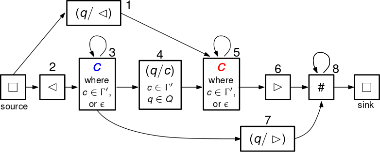
Lemma 6.5
[Properties of a Valid Row in Layer ] A row is valid if and only if the row satisfies the following conditions:
- 1.
The tape contents of the row has the form:
- 2.
There is exactly one tile is a head tile.
- 3.
The head is located at one of the tiles from the to the .
- 4.
Any tiles from to the left of the head tile are blue and any tiles from to the right of the head tile are red.
Proof: Any path in the graph in Figure 11 must pass through vertex , , or exactly once and therefore has exactly one head tile. In addition, the path goes through or , then vertices from , , and , followed by one of vertices or and then vertex . Therefore, the tape contents of each such path must have the form . There are no vertices in the graph in which the head is located at a or tile, so the head must point to one of the symbols between the and tiles. If vertex is reached, then it comes before vertex or , which means that all the blue tiles from precede the head tile. If vertex is reached, then it comes after vertex or , which means that all the read tiles from come after the head tile.
For the converse, consider a row that satisfies all the properties in the lemma. If the head points to the symbol, then it can be generated by a path of the form . If the head points to the a symbol from , then it can be generated by a path of the form . If the head points to the symbol, then it can be generated by a path of the form .
We describe the Turing Machine rules in the next section. It will be important that there is a unique next step for any Turing Machine configuration that corresponds to a valid row.
6.4.3 The Layer 3 Turing Machine
The Turing Machine in Layer 3 is global in the sense that it works across all the intervals. The tape alphabet is the set:
The symbols in are called marked digits. For digit , marking corresponds to replacing with and unmarking corresponds to replacing with . Other than marking or unmarking digits, the Turing Machine never changes the information on the tape.
The program of the Turing Machine consists of two nested loops. The TM will just continually run the Outer Loop for as many steps as it is allowed to run. Consider the row at the beginning of an iteration of the Outer Loop. Let be the locations of the tiles in this row. For each such tile, let be the string of digits immediately to the right of the tile. Note that could be the empty string if is followed by a non-digit. If the Outer Loop is executed without error, there will be a cost in an iteration of the Outer Loop for each , where and .
The digits in each string that have already been checked are marked. In an iteration of the Inner Loop, the Turing Machine reads the first unchecked digit in and checks that digit against the first unmarked digit in each of the other ’s. When a digit is checked, it becomes marked.
Figure 12 shows the steps of the Outer Loop in pseudo-code. Figure 13 gives a table with all the Turing Machine rules. An iteration of the Outer Loop begins with the head just one space to the left of . The Turing Machine sweeps left, unmarking all the digits until is reached. This begins an iteration of the inner loop. The head sweeps right all the way from to , starting in state . When the first is encountered, the Turing Machine reads and remembers the next unmarked digit and transitions to . This is the next unchecked digit of . The digit is checked. In state the head is looking for an which indicates the beginning of the next . After an is reached, it transitions to indicating that it is looking for the next unmarked digit. When the next unmarked digit is found, it checks if . If , a cost is incurred. The digit is marked and the head transitions to in order to look for the next . The Turing Machine also incurs a cost if in state and a non-digit is encountered, indicating that the current being checked is shorter than . When the is reached, then the Turing Machine transitions to and sweeps left to the to begin a new iteration of the inner loop. The Outer Loop terminates when all the digits in have been checked. This happens, when the state is and the head encounters a non-digit before an unmarked digit. The head then transitions to and sweeps right to the . While the Turing Machine is in state , any unchecked digit causes the Turing Machine to incur a cost. This happens is one of the strings is longer than . When the head reaches , it transitions to which begins a new iteration of the Outer Loop.
(1) OuterLoop: (3) Sweep left in state , unmarking every digit. (4) When is reached, transition to and move right (5) Start of Inner Loop (6) Move right in state until an or is reached (7) If is reached before , transition to . Go to (1). (8) When is reached, transition to (9) Move right in state past any marked digits (10) If is reached before a digit, go to (24) (11) If is reached before a digit, go to (26) (12) If unmarked digit is reached, mark , transition to . (13) Move right in state until an or is found. (14) If is reached, go to (22). (15) If is reached, transition to . (16) Move right in state past any marked digits. (17) If an unmarked digit is reached, mark and transition to . (18) If , then Cost. (19) If non-digit is reached for any , transition to . Cost. (20) If is reached, stay in . Cost. (21) If is reached, go to (22). Cost. (22) Transition to . Move left until is found. (23) Transition to . Go to (5) (24) Transition to state , move right until is reached (25) If an unmarked is encountered in state , there is a Cost. (26) Transition to . Go to (1).
| Right | Right | |||
| Right | Right | Right | Right | |
| Right | ||||
| Right | Right | |||
| Right | Right |
| Left | Left | ||
| Left | Right | ||
| Left | Right | Left | |
| Right | |||
| Left | Left | ||
| Left | Right | Left |
The Turing Machine rules are translated into legal and illegal computation squares for as described in Section 2.2. As with Layer , a legal head square is legal as long as any tiles from to the left of a head tile is blue and any tiles from to the right of a head tile are red. Also, a square is illegal if it has a tape tile directly above another tape tile that are different in any way, including the color.
There is one final type of illegal square which occurs only in Layer . These introduce the costs indicated in the pseudo-code shown in Figure 12. Any square which contains a tile of the form where or , where , is an illegal square. In addition, any square that contains where is also an illegal square. We will call these illegal verification squares.
Lemma 6.6
[Sequential Rows Represent TM Steps in Layer ] Consider a row that is valid in Layer . There is a unique row that can be placed above such that there are no illegal computation squares that span the two rows and . is valid. Moreover, row corresponds to a Turing Machine configuration and represents the configuration resulting from executing one step in the configuration .
Proof: Consider a valid row . If there is a row such that if is placed directly above , there are no illegal computation squares, then must be unique. The argument is almost identical to the analogous lemma proved for the Layer Turing Machine given in Lemma 3.2.
Next we need to show that if is valid, then there is a valid such that there are no illegal computation squares spanning rows and . Since is valid, there is exactly one head tile in and therefore corresponds uniquely to a configuration of the Turing Machine. Let be the row resulting from applying one step of the Turing Machine to the configuration represented by row . Color all the tiles to the left of the head tile blue and all the tiles to the right of the head tile red.
We will first establish that there are no illegal squares spanning rows and . The head square must be legal because it represents one correctly executed step of the Turing Machine. All other tiles outside of the head square are tape tiles and are the same in and because they did not change in the computation step. Moreover since is valid, all tiles to the left of the head square are blue and all tiles to the right of the head square are red. Therefore any tiles outside of the head square have the same color in and .
To establish that is valid, we will show that has all the properties from Lemma 6.5. If the head is pointing to a symbol, it writes a and moves right. If the head is pointing to a symbol, it writes a and moves left. If the head is pointing to a symbol from , it writes a symbol from and moves left or right. This guarantees properties through . Property is guaranteed by construction.
6.4.4 Analysis of Layer
We would like to argue that if the number of illegal pairs or squares in Layer is less than a certain value, then there will be a complete error-free iteration of the Outer Loop.
Definition 20
[End Row for Layer ] An end row for Layer is a valid row in which the head is pointing to symbol in state or .
Note that since an end row is valid, it corresponds to a valid configuration of the Turing Machine. In the next next step of the Turing Machine, the head is just to the left of the symbol in state , which begins a new iteration of the Outer Loop.
Lemma 6.7
[Number of Steps to Reach an End Row in Layer ] Consider a valid row in Layer of a tiling. Let be the maximal string of digits to the immediate right of the left-most tile in . If there is no tile, then is empty. If rows through are all valid and do not contain any illegal computation squares and , then one of the rows in through must be an end row.
Proof: We will argue that if the Turing Machine starts in a valid configuration, then it will reach an end configuration within steps.
Each iteration of the Inner Loop begins with the head just to the right of the symbol in state . We will first establish that it takes at most steps to reach the beginning of an iteration of the Inner Loop or an end configuration. If the state of is or , the head moves left until a symbol is reached. Then the head moves right into state , for a total of at most steps. If the state of is , , , or then the head will continue moving right and remain in one of those states until the is reached. If the state is , or when the is reached, this is an end configuration. If the state is or when the is reached, the Turing Machine will move left in state until the is reached, at which point it transitions to and moves right. This is the beginning of an iteration of the Inner Loop. The total number of steps so far has been .
If the Turing Machine starts an iteration of the Inner Loop and the head never reaches an in state , it will reach the symbol in state , which is an end configuration. In this case, and the number of steps spent in the Inner Loop is . Otherwise, the head will eventually reach an and will transition to . If the head reaches a digit before a symbol from in state , the digit will be marked and the head will continue going right in state or until it hits the symbol, in which case it transitions to , sweeps left until the symbol is reached and then moves right into to start another iteration of the Inner Loop. The marked digit is part of because at the beginning of an iteration of the Inner Loop, the state is initially and can only transition to when the first is reached. The state remains in state until a symbol from or a digit is reached. Thus, if a digit is reached before a symbol from m the current string is still . Therefore, in each iteration of the inner loop, one additional digit from becomes marked and there can be at most iterations of the inner loop, each of which takes at most steps. The Inner Loop Iterations take a total of at most steps.
Finally, if the state is and the Turing Machine reaches a symbol from , it will sweep right in state (if it is not already at the symbol) until the is reached. Within an additional steps, the head will reach in state or , which is and end configuration. The total number of steps is at most .
The set is the set of digits in . We can augment to include the marked digits as well: . The function maps strings in to strings in by changing marked digits to the corresponding unmarked digits, so is mapped to . The functions and can be extended to strings from by first applying the function and then applying or .
Lemma 6.8
[Bound on the Length of a String of Digits in Layer ] Let be any row in Layer of a tiling of an grid. Let be a string of consecutive tiles from in . Then
Proof: Consider a sequence of consecutive tiles in locations through that are all from , where . If locations through in the last row in Layer are either bits ( or ) or head tiles with bits ( or ) then by Lemma 6.3, there is an illegal square contained in locations through spanning two consecutive rows in Layer . If the last row of Layer , locations through contain a tile that is not , , , or , then either there is an illegal translation square contained in those locations or those locations contain a tile that is not from the set in the first row of Layer . Furthermore, any two vertically aligned tiles in Layer in which a tile not from is directly below a tile that is from prime must be contained in illegal squares on both sides. Therefore, if the locations through contain tiles from in a row from Layer , then those locations must contain an illegal square somewhere in Layers or . Partition the locations of into consecutive locations of length . There must be an illegal square from Layers or contained within each set of locations, which means that there can be at most sets of locations. Therefore the length if is at most .
Lemma 6.9
[Layer Completes At Least One Iteration of the Outer Loop] As long as and , there is a sequence of rows in Layer with no illegal pairs or computation squares, in which the Turing Machine executes a complete iteration of the Outer Loop.
Proof: Consider a set of consecutive rows in Layer with no illegal pairs or computation squares. Let be the first row in the sequence or rows. Let be the maximal sequence of tiles in row from the set that are directly to the right of the leftmost tile in row . By Lemma 6.7, if the sequence lasts for at least rows, then the computation represented in the sequence of rows will reach the end of an iteration of the Outer Loop. Note that and do not change in the course of these rows because there are no illegal computation squares and the computation does not change the contents of the Turing Machine tape other than marking or unmarking digits. Thus, if the sequence lasts for yet another rows, then the computation represented in the sequence of rows will include one full iteration of the Outer Loop. So as long as the sequence contains at least rows, it will be guaranteed to contain a complete iteration of the Outer Loop with no computation errors.
Lemma 6.2 gives an upper bound on the length of the last row of Layer which for now we will call . Any two vertically aligned tiles with a non- tile on top of a tile will be contained in illegal computation squares on both sides. So the length of row can be at most the upper bound from Lemma 6.10 plus . Meanwhile, Lemma 6.8 gives an upper bound of for . Putting these bounds together means that if we are guaranteed to have a sequence of at least
consecutive rows with no illegal squares or computation squares, then there will be a complete iteration of the Outer Loop with no computation errors.
Besides the first and last rows which are all filled with tiles, there are a total of rows. There are at most rows with an illegal pair or square. Therefore there must be at least one sequence of at least rows with no illegal pairs or squares. So as long as the following inequality holds:
If , then the bound from Lemma 6.2 says that . Using the assumption from the Lemma that , the inequality above can be verified.
Lemma 6.10
[Summary of Analysis of Layer ] Consider a tiling of an grid, where , for some binary string . Let be the total number of illegal squares and pairs in Layer , for . At the end of Layer , the following conditions hold:
- 1.
If is the set of sizes of clean intervals in the last row of Layer , then .
- 2.
Every clean short-form interval at the end of Layer has the form , or .
- 3.
Any clean interval of size at least is a long-form interval.
- 4.
If and , then there exists a such that every long-form clean interval of has the form , where and and .
Proof: Let be the set of tags corresponding to clean intervals in the last row of Layer . Let be the set of tags corresponding to clean intervals in the last row of Layer . Since no clean intervals are created from the last row of Layer to the last row of Layer and each clean interval adopts the same tag as the corresponding clean interval in the preceding row, . If there is a clean interval in the last row of Layer with tag and no such clean interval in the first row of Layer , then the interval contains an illegal translation square. Similarly, a clean interval with tag that does not correspond to a clean interval with tag in the next row, must contain an illegal square. Since every lost clean interval corresponds to an illegal translation square or illegal computation square in Layer , . If is the set of sizes of clean intervals at the end of Layer m then by Lemma 6.2, . At most clean intervals are lost from the end of Layer to the end of Layer . Therefore, .
Item follows from the fact that the Turing Machine in Layer does not change any tile from one row to another, except for the movement of the head and marking or unmarking digit tiles. Therefore, if an interval is clean in Layer , it has the same form as it did in the first row of Layer . Lemma 6.4, indicates what the short-form and long-form intervals look like in the first row of Layer . Also, the intervals do not switch between being long-form or short-form intervals from the last row of Layer . Therefore, by Lemma 6.2, any clean interval of size at least must be a long-form interval in the last row of Layer , which proves item .
Now to prove item . The assumption for this Lemma are the same as the conditions for Lemma 6.9, so there is a sequence of consecutive rows in Layer that do not contain any illegal pairs or computation squares that correspond to a complete iteration of the Outer Loop. The be the first row in this sequence. Find the location of the leftmost tile in and let be the maximal sequence of consecutive tiles from that are immediately to the right of the tile. After the head sweeps left in state at the beginning of the Outer Loop, every clean interval has the form , where . Each corresponds to the clean interval as they are numbered from left to right. may or may not be the same as .
If there is an where digit of differs from digit of , then on the iteration of the inner loop, there will be an illegal verification square in interval when the Turing Machine is in state and the first unmarked digit in interval is . This occurs in line of the pseudo-code in Figure 12. Otherwise, if , then must be a proper prefix of or is a proper prefix of . If is be a proper prefix of , in the last iteration of the Inner Loop, when there are no longer unchecked digits in , there will remain unchecked digits in . These will trigger an illegal verification square when the Turing Machine is in state and encounters the unchecked digit in interval . Finally if is a proper prefix of , after iterations, the Turing Machine will read digit of but will encounter no unmarked digits in interval . The state will transition to when it reaches the in interval and it will encounter a non-digit before it encounters an unmarked digit. Thus triggering a cost in Line in the pseudo-code.
Thus, every interval such that will no longer be clean after the iteration of the Outer Loop. Since every clean interval started with , and the string of digits in the interval does not change as long as the interval remains clean, then will remain true after the iteration of the Outer Loop. In the remainder of the rows, if the interval remains clean, then it contains no illegal computation squares and the string of digits remains the same, except perhaps that some digits become marked, so Item will still hold for the last row of Layer .
6.5 Layer
The translation rules from Layer to Layer translate any or tile to , for . is translated to , and is translated to for any . The states from Layer are all dropped, so any tile of the form is translated to whatever would be translated to, according to the rules above. These translation rules ensure that every clean interval is translated to a clean interval as long as the tiles in the interval are translated correctly. Thus every clean long-form interval has the form: .
Recall that the functions and map a string of length over to two binary strings of length . The variable will denote the binary string with the last bit removed and will denote . will be used as the input to the computation and will be used as a guess of the answers to the queries to the oracle . We will use to denote the number of oracle queries made by on input , so we will only be concerned with the first bits of .
The tiling rules in Layer enforce that an tile must have a or tile above and below it. Similarly for and , so the only tiles that change from one row to another are tiles inside long-form interval unless there is an illegal square. Every clean long-form interval will contain an independent Turing Machine computation. The Turing Machine rules are translated into legal and illegal squares as described in Section 2.2. If the head reaches the at the right end of the interval, then the interval is not wide enough to complete the computation. In this case, the computation halts and does not incur any additional cost.
The definitions for clean and corrupt intervals carry over to Layer as well. Since clean intervals do not change locations within a row, two clean intervals will have the same tag and long/short-form designation if they occupy the same locations within their respective rows. An interval in the first row of Layer is clean if those tiles corresponded to a clean interval at the end of Layer and the interval does not contain any illegal translation or initialization squares. In going from one row to the next row in the computation in Layer , an interval is clean if those tiles corresponded to a clean interval in the previous row and there are no illegal squares spanning the current and previous rows in the interval.
Lemma 6.11
[Bound on the Missing Clean Interval Sizes] Let be the total number of illegal squares and pairs in Layer , for . If is the set of clean intervals at the end of Layer then .
Proof: Let be the set of tags corresponding to clean intervals in the last row of Layer . Let be the set of tags corresponding to clean intervals in the last row of Layer . Since no clean intervals are created from the last row of Layer to the last row of Layer and each clean interval adopts the same tag as the corresponding clean interval in the preceding row, . If there is a clean interval in the last row of Layer with tag and no such clean interval in the first row of Layer , then the interval contains an illegal translation square. Similarly, a clean interval with tag that does not correspond to a clean interval with tag in the next row, must contain an illegal square. Since every clean interval that is lost in Layer corresponds to an illegal square in Layer , . If is the set of sizes of the clean intervals at the end of Layer , then by Lemma 6.10, . Since at most clean intervals are lost from the end of Layer to the end of Layer , .
6.5.1 The Layer Computation
Recall that we are reducing from a generic language to Function Weighted Tiling. denotes the poly-time Turing Machine that computes with access to a NEXP oracle. is the the NEXP-time language that is the oracle for . denotes the -time Turing Machine that is the verifier for .
The reduction maps a string to an integer such that after steps of the Binary Counter Turing Machine described in Section 5.1, the string on the tape is and the head is at the left end of the tape. According to Lemma 5.3, , where is the reverse of string , is the numerical value of the string in binary, and is the number of ’s in .
All the clean long-form intervals start out with configuration
The computation that is initiated by state proceeds in several stages.
Stage 1: The computation in Stage ”measures” the size of the interval and writes the size of the interval in binary. This is accomplished by a counter similar to the one used in [GI13]. The Turing Machine uses a binary and a unary counter. The head shuttles back and forth between the two ends of the interval (using the and the tiles to know when it has reached one of the two ends). In each cycle, the head increments both counters. When the unary counter has reached the on the right end of the interval, it transitions to a new state which begins the next phase of the computation. The counting procedure actually counts the number of interior tiles in the interval and the definition of the size of an interval includes the two endpoint tiles, so we add to the final count to get the size of the interval. We will call this value for a particular interval. Note that a clean interval can increase in size by at most per segment, so the size of any clean interval is bounded by the number of segments, which by Lemma 4.12, is . We will argue below that the cost of the minimum tiling, which is at least is . As long as the size of a clean interval is , this phase of the computation takes time .
Stage 2: The next stage of the computation uses , , and to select a term in the cost function towards which it will contribute. Recall that is an upper bound on the number of oracle queries made by on an input of length . The bit of will be denoted by . The goal will be to have intervals checking the bit of , where
From the string , the size of the grid is computed, as is the number of intervals after steps of a correct computation of the Layer Turing Machine. The time and space complexity of the computation in Stage is bounded by a polynomial in , which is polylogarithmic in . By Lemmas 5.3 and 4.25, given of length , the values of and can be computed in time, which is polylogarithmic in .
The output of the function on input with oracle responses is denoted by which is also computed by the Turing Machine. Note that in the idealized case in which the interval sizes go from down to , the value is an almost unique identifier for each interval going from up to from left to right. Note that even in a fault-free computation, if the computation in Layer finishes in the middle of an iteration of the Outer Loop, the sequence of interval sizes will deviate slightly from the idealized case. The computation in each interval will perform different tasks, depending on the value of .
| Value of | Action Taken |
|---|---|
| Transition to and halt | |
| Compute the bit to check | |
| as described below | |
| Go to Stage | |
| Transition to and halt | |
| Transition to and halt |
There is a cost of for any computation square that enters a state, so rejecting computations incur a cost of exactly . Accepting computations do not incur any cost. The value of is defined to be the smallest index such that
In the next stage, the computation (if it did not stop in Stage ) will check the bit of .
Stage 3: If , then the TM transitions to and halts. If , then the TM simulates the Turing Machine until the point of the query, using as the oracle responses for the first oracle queries. Let be the input to the oracle query. The computation now simulates the verifier on input using a witness that is guessed. If accepts, the cost is and if rejects the cost is . If , there is a witness that causes to accept , which implies that there is a -cost tiling of that strip in Layer . If , then any tiling will either have an illegal square because the TM was not correctly executed or will have a cost of when terminates.
6.6 Putting the Layers Together
The costs for computations are realized by having any legal computation square which transitions to have a cost of . We will call these rejecting squares in order to distinguish them from illegal squares which in general have a higher cost. We are finally ready to define the cost of a square over all four layers of the tiling. Consider a square of four tiles where each tile is described by it’s tile type for each later. Let denote the indicator variable that is if the Layer tile types are an illegal square for Layer , and is otherwise. Let and designate if the square has an illegal pair in its bottom two tiles for Layers and . Let be an indicator variable denoting whether the square is a rejecting square in Layer . The cost of the square is:
Thus if is the number of illegal pairs or squares in Layer , and if is the number of rejecting squares in Layer , the total cost of a tiling is
is the cost from illegal pairs and squares. We will call the rejection cost for the tiling.
We need to establish that regardless of whether , the minimum cost tiling has no illegal pairs or squares and the choice of corresponds the correct oracle responses for the queries to language . We first establish an upper bound on the minimum cost tiling of an grid.
Lemma 6.12
[Upper Bound on the Minimum Cost of a Tiling] There is a tiling of the grid whose cost is at most .
Proof: Consider a tiling with no illegal pairs or squares in which the string used for the oracle output bits is all ’s. According to Lemma 4.24, the sizes of the intervals are contained in with at most one duplicate. Let . The leftmost intervals will incur a cost of since all the query responses are assumed to be . The other intervals will not incur any cost. Since there can be at most one duplicate in the range , the total cost will be at most . The highest order bit of is in location . Therefore, the highest order bit of is and the value of is at most , which by Claim 6.1 for large enough can assumed to be at most .
Lemma 6.13
For sufficiently large , the minimum cost tiling has at least one clean long-form interval at the end of Layer .
Proof: If is the set of sizes of clean intervals in the last row of Layer , then Lemma 6.11 says that . By Lemma 4.25, the value of is at least . If the tiling has a minimum cost then by Lemma 6.12,
Therefore . By Lemma 6.10, any clean interval of size at least is a long-form interval. Therefore for large enough , there is at least one long-form interval.
Any tiling in which , the number of illegal pairs or squares in Layer , is greater than will have cost at least since each illegal pair or square in Layer contributes to the overall cost. We know from Lemma 6.12 that such a tiling will not be a minimum cost tiling. Therefore, we can ignore those tilings and assume that the condition in Item of Lemma 6.10 are met. This implies that there is a single in every clean long-form interval at the end of Layer . Define to be the cost of the minimum cost tiling whose clean large-form intervals all have string and that have illegal pairs or squares.
The following Lemma says that we can ignore tilings with illegal pairs or squares.
Lemma 6.14
For every , and every , .
Proof: Fix the string . Let be a minimum cost tiling with string and illegal squares. Similarly for . Let denote the number of illegal squares on Layer in . We only know that at least one of the ’s is positive. The cost of from illegal squares is . The cost of from illegal squares is . Let denote the rejection cost of tiling . We will prove that .
Let be the the lengths of the clean intervals in the last row of Layer for . Any clean interval of size in incurs exactly the same cost as a clean interval of size in . Because the intervals are clean, the computations inside those intervals is the same and correct. Since the size of the interval is the same, the value of and for the two intervals is the same. Therefore the bit of that is checked in the interval is the same. Since and are both assumed to be minimum cost tilings, the best witness for each computation in Layer is chosen. In other words, if there is a -cost tiling for that interval, it will be used in both and .
If has intervals, those intervals will all have sizes in the range through . Furthermore, according to Lemma 4.24, there is only one number in that range such that has two intervals of that size. This one extra interval will contribute a cost of at most to the overall cost. If is the set of sizes of the clean intervals at the end of Layer in , then the difference in rejection costs between and is at most .
We can now focus on tilings that have no illegal squares.
Lemma 6.15
In any tiling with no illegal squares, the largest intervals will be wide enough to complete their computations, where .
Proof: Suppose input string maps to the number in the reduction. According to Lemma 4.25, the number of intervals at the end of Layer is at least . The largest of these intervals have size at least . By Claim 6.1, any of these intervals will be large enough to complete a computation of the verifier . All the other computations in Layer as well as the other layers are polynomial in and therefore polylogarithmic in .
We need to establish that so that the intervals used in the computation are among the largest. The value of is maximized if the string is all ’s. In this case the value of is at most . By Claim 6.1, we can assume that .
Let be the number of intervals that check the bit of . The goal is to have . Let be the number of intervals whose value is in the range through . The goal is to have . The following lemma shows that actual values for the num functions are not far from the goal.
Lemma 6.16
For any , in a fault-free tiling:
Proof: The set of interval sizes that check the bit are exactly those for which is in the range
The value of are the number of intervals with size such that is in the range
Note that all of the above ranges are disjoint and contained in . If the multi-set of all for all the intervals is exactly through , then for every , is exactly and . According the Lemma 4.24, the multi-set of interval sizes for a correct computation is contained in . Moreover, there are at most two integers missing from this range and at most one duplicate. The Lemma follows.
Let be a string such that and , where is the correct answer to all of the oracle queries made by to the oracle on input . Note that the string may not be unique because the number of oracle calls is less than , the number of bits in , so bits through of can be arbitrary.
Lemma 6.17
Consider a tiling of an grid, where , for some binary string . Let be a string such that and , where the bit of is the correct answer answer to the oracle query, for . For every , .
Proof: By Lemma 6.10, in the last row of Layer every clean long-form interval has a such that . Since the translation rules preserve the string, then any clean interval in the first row of Layer will also have .
Let be the number of oracle calls made by Turing Machine on input . We need to establish that the minimum is achieved when the first bits of are the same as the first bits of .
By induction. Assume that we have established that the first bits of the minimum must match in order to achieve the minimum cost. The inputs to the first oracle queries are now fixed. Call these . Now suppose that . That means . Any string that agrees with in the first bits and has , will pay a cost of which is at least . Suppose instead we use the string that has followed by a string of zeros. The intervals that are checking bit can be tiled at cost because is in fact in . The intervals that are checking bits through as well as the intervals implementing the cost will incur a cost of which by Lemma 6.16, is at most
Since this is less than the cost of the incorrect guess , the incorrect guess for can not yield the minimum cost when the correct guess .
Now suppose that . That means . Any string that agrees with in the first bits and has , will pay a cost of which is at least . Note that since , when the verifier is run on input , it must reject, which means that the intervals that check bit will incur a cost of . Suppose instead we use and ’s for the remaining bits of . The cost will be which by Lemma 6.16, is at most
Since this is less than the cost of the incorrect guess , the incorrect guess for can not yield the minimum cost when the correct guess .
We have shown that regardless of the true value for , an incorrect guess for will result in a higher cost than the correct guess.
We now have all the pieces in place to prove the reduction.
Theorem 6.18
Consider a tiling of an grid, where , for some binary string . Then the value of can be recovered from the cost of the minimum cost tiling of an grid.
Proof: By Lemmas 6.14 and 6.17, the minimum cost tiling does not have any illegal pairs or squares and guesses a that maps to the correct for the input and the correct for the oracle responses. The overall cost of the tiling will be
According to Lemma 6.16, the value will be one larger or two smaller than
By dividing the minimum cost tiling by and rounding to the nearest integer, the lowest order bits will be the value of .
7 Parity Weighted Tiling
The construction for Parity Weighted Tiling is almost exactly the same as with Function Weighted Tiling. We slightly modify the translation of intervals from Layer to Layer as follows. The translation rules from Layer to Layer translate any or tile to , for . is translated to or , and is translated to for any . The states from Layer are all dropped, so any tile of the form is translated to whatever would be translated to, according to the rules above. These translation rules ensure that every clean interval is translated to a clean interval as long as the tiles in the interval are translated correctly. Thus every clean long-form interval has the form: . The ambiguity in whether is translated to or is resolved by the translation rule that must be translated to and must be translated to . Thus the leftmost interval (if it is a clean long-form interval) looks like and every other clean long-form interval looks like .
We are now reducing from a language which is computed by a polynomial time Turing Machine with access to a NEXP oracle. All intervals except for the leftmost interval behave in exactly the same way as for the function version, except that they incur a cost of for entering a rejection state. Note that we can think of the function for the decision problem as just mapping to a single bit, depending on whether accepts or rejects. The computation in the leftmost interval starts in a different start state which indicates that it will simulate the Turing Machine on input and incur a rejection cost of depending on whether accepts or not.
Finally multiply the cost of an illegal pair or square from the Function Weighted Tiling construction by . Note that all costs, except the cost of the computation in the leftmost interval are all a multiple of times their corresponding cost in the Function Weighted Tiling construction, so the analysis in Section 6 comparing costs of different tilings still holds.
Theorem 7.1
Consider a tiling of an grid, where , for some binary string . Then the minimum cost tiling of an grid is odd if and is even if .
Proof: By Lemmas 6.14 and 6.17, the minimum cost tiling does not have any illegal pairs or squares and guesses a that maps to the correct for the input and the correct for the oracle responses. Since the string is the same in all the long-form intervals, the the leftmost interval has the correct input and the correct outputs to the oracle queries. All costs in the tiling are even, except for the penalty at the end of the computation of the leftmost interval. This computation will accept if and only if . If the computation accepts, the cost in this interval is and the overall cost of the minimum cost tiling is even. If the computation rejects, then the cost in this interval is and the cost of the entire tiling is odd.
8 Acknowledgements
We are grateful to the Simons Institute for the Theory of Computing, at whose program on the “The Quantum Wave in Computing” this collaboration began.
References
- [AGIK09] Dorit Aharonov, Daniel Gottesman, Sandy Irani, and Julia Kempe. The power of quantum systems on a line. Communications in Mathematical Physics, 287(1):41–65, Jan 2009.
- [AI21] Dorit Aharonov and Sandy Irani. Hamiltonian complexity in the thermodynamic limit. arXiv:2107.06201, 2021.
- [Amb14] Andris Ambainis. On physical problems that are slightly more difficult than qma. In 2014 IEEE 29th Conference on Computational Complexity (CCC), pages 32–43, 2014.
- [Bah82] F Baharona. On the computational complexity of ising spin glass models. Journal of Physics A: Mathematical and General, 15(10):3241–3253, 1982.
- [BCO17] Johannes Bausch, Toby Cubitt, and Maris Ozols. The complexity of translationally invariant spin chains with low local dimension. Annales Henri Poincaré, 18(11):3449–3513, Oct 2017.
- [CPGW15] Toby S. Cubitt, David Perez-Garcia, and Michael M. Wolf. Undecidability of the spectral gap. Nature, 528(7581):207–211, Dec 2015.
- [GHLS15] Sevag Gharibian, Yichen Huang, Zeph Landau, and Seung Woo Shin. Quantum hamiltonian complexity. Foundations and Trends® in Theoretical Computer Science, 10(3):159–282, 2015.
- [GI13] Daniel Gottesman and Sandy Irani. The quantum and classical complexity of translationally invariant tiling and hamiltonian problems. Theory of Computing, 9(2):31–116, 2013.
- [GPY19] Sevag Gharibian, Stephen Piddock, and Justin Yirka. Oracle complexity classes and local measurements on physical hamiltonians. arXiv:1909.05981, 2019.
- [GY19] Sevag Gharibian and Justin Yirka. The complexity of simulating local measurements on quantum systems. Quantum, 3:189, September 2019.
- [Ist00] Sorin Istrail. Statistical mechanics, three-dimensionality and np-completeness. i. universality of intractability for the partition function of the ising model across non-planar lattices. pages 87–96, 01 2000.
- [Kre86] Mark W. Krentel. The complexity of optimization problems. In Alan L. Selman, editor, Structure in Complexity Theory, pages 218–218, Berlin, Heidelberg, 1986. Springer Berlin Heidelberg.
- [KSV02] A. Yu. Kitaev, A. H. Shen, and M. N. Vyalyi. Classical and Quantum Computation. American Mathematical Society, USA, 2002.
- [OT05] R. Oliveira and B. Terhal. The complexity of quantum spin systems on a two-dimensional square lattice. arXiv:0504050, 2005.
- [Pap94] Christos H. Papadimitriou. Computational complexity. Addison-Wesley, 1994.
- [Rob71] Raphael Robinson. Undecidability and nonperiodicity for the tilings of the plane. Invent. Math., 12:177–209, 1971.
- [Wan60] Hao Wang. Proving theorems by pattern recognition. Communications of the ACM, 3(4):220–234, 1960.
- [WBG20] James D. Watson, Johannes Bausch, and Sevag Gharibian. The complexity of translationally invariant problems beyond ground state energies. arXiv:2012.12717, 2020.
- [WC21] James D. Watson and Toby S. Cubitt. Computational complexity of the ground state energy density problem. arXiv:2107.05060, 2021.