Parallel window decoding enables scalable fault tolerant quantum computation
Abstract
Large-scale quantum computers have the potential to hold computational capabilities beyond conventional computers for certain problems. However, the physical qubits within a quantum computer are prone to noise and decoherence, which must be corrected in order to perform reliable, fault-tolerant quantum computations. Quantum Error Correction (QEC) provides the path for realizing such computations. QEC continuously generates a continuous stream of data that decoders must process at the rate it is received, which can be as fast as 1 MHz in superconducting quantum computers. A little known fact of QEC is that if the decoder infrastructure cannot keep up, a data backlog problem Terhal 2015 is encountered and the quantum computer runs exponentially slower. Today’s leading approaches to quantum error correction are not scalable as existing decoders typically run slower as the problem size is increased, inevitably hitting the backlog problem. That is: the current leading proposal for fault-tolerant quantum computation is not scalable. Here, we show how to parallelize decoding to achieve almost arbitrary speed, removing this roadblock to scalability. Our parallelization requires some classical feed forward decisions to be delayed, leading to a slow-down of the logical clock speed. However, the slow-down is now only polynomial in code size, averting the exponential slowdown. We numerically demonstrate our parallel decoder for the surface code, showing no noticeable reduction in logical fidelity compared to previous decoders and demonstrating the parallelization speedup.
Quantum error correction (QEC) generates a stream of syndrome data to be decoded. An offline decoder collects and stores all the syndrome data generated during a hardware run (often called a shot) and then performs decoding as a post-processing step. Offline decoding is sufficient for computations consisting solely of Clifford gates (e.g. CNOT and Hadamard gates). However, fault-tolerant quantum computations must adapt in response to certain logical measurement results, which must be decoded to be reliable. For instance, when performing gates using teleportation and a magic state Bravyi and Kitaev 2005; Litinski 2019, we must decide whether to apply a Clifford correction before performing the next non-Clifford operation (see Fig. 1). This logic branching decision can only be reliably made after we decode the syndrome data from the gate teleportation DiVincenzo and Aliferis 2007; Terhal 2015; Chamberland et al. 2018. Therefore, online, or real-time, decoding is necessary for useful quantum computation. Classical computation occurs at finite speed, so online decoders will have some latency, but they need only react fast enough to enable feed-forward and Clifford correction.
How fast do decoders need to be? A fundamental requirement was first noted by Terhal Terhal 2015 in her backlog argument
“Let be the rate (in bauds) at which syndrome bits are processed and be the rate at which these syndrome bits are generated. We can argue that if , a small initial backlog in processing syndrome data will lead to an exponential slow down during the computation, …”
Terhal proved that quantum algorithms with -depth have a running time lower bounded by when and is some constant. Refs. Holmes et al. 2020; Chamberland et al. 2022a provide more detailed reviews of this backlog argument. However, for all known decoders, as we scale the device decoding becomes more complex, the value of increases and inevitably we encounter the backlog problem.
Here we solve this problem, removing a fundamental roadblock to scalable fault-tolerant quantum computation. We propose parallelized window decoding that can be combined with any inner decoder that returns an (approximately) minimum weight solution, presenting results for minimum-weight perfect matching (MPWM) Dennis et al. 2002; Fowler et al. 2009; Higgott 2021 and union-find (UF) Delfosse and Nickerson 2021; Das et al. 2020.
The previous leading idea was to modify decoders to work online was proposed by Dennis et al Dennis et al. 2002:
“take action to remove only these long-lived defects, leaving those of more recent vintage to be dealt with in the next recovery step.”
Here defects refer to observed changes in syndrome. Dennis et al called this the overlapping recovery method Dennis et al. 2002; Huang and Brown 2021. Later, similar approaches were adopted for decoding classical LDPC codes Iyengar et al. 2012, where this is known as sliding window decoding. Roughly speaking, given a sequence of defects proceeding in time one decodes over some contiguous subset, or window. The decoder output gives only tentative error assignments, and from these only a subset — those of an older vintage — are ‘committed’. Here, committing means making a final correction decision for potential error locations, with all corrections performed in software. One then slides the window up and the process repeats.
Sliding window decoding is inherently sequential. Let us consider a single code block (e.g. a surface code patch) with each QEC round taking seconds. If each window is responsible for committing error corrections over rounds of syndrome data, then it takes time to generate all this data. If the time to decode each window is , including any communication latency, then avoiding Terhal’s backlog problem requires that . Since typically grows superlinearly with the decoding volume, this leads to a hard upper bound on the achievable distance . For example, a distance surface code has and therefore we are restricted to . Scaling hardware based on a fixed device physics means is fixed. This imposes a hard limit on code distance. The reader should pause to reflect how remarkable it is that the current leading proposal for fault-tolerant quantum computation is not scalable.
As with sliding window decoding, our parallel window decoder breaks the problem up into sets of overlapping windows. Rather than solving these sequentially, some windows are decoded in parallel by adapting how overlapping windows are reconciled. Through numeric simulations, we find that sliding, parallelized and global approaches differ in logical error rates by less than the error bars in our simulations. We show that, by scaling classical resources, parallel window can achieve almost arbitrarily high regardless of decoding time per window . Furthermore, we show that while there is still an inherent latency determined by leading to a slow-down of the logical clock speed, this is only linear in , rather than the exponential slow down resulting from Terhal’s backlog argument. We conclude with a discussion of the implications of this work for practical decoder requirements and extensions to a number of other decoding problems. After making this work public, similar results were posted by the Alibaba team Tan et al. 2022. The Alibaba numerics present the logical fidelity of the decoder, but do not include numerical results on decoding speed and improvements through increasing number of processors used.
I Results and Discussion
I.1 Matching decoders
Windowing techniques, both sliding and parallel, can be combined with most decoders acting internally on individual windows. We will refer to these as the “inner decoders”. However, for brevity, in the main text we will describe the procedure for the case of matching decoders, such as MWPM and union-find. A matching decoder is applicable when any error triggers either a pair of defects or a single defect. For example, in the surface code errors lead to pairs of defects (when occurring in the bulk) or a single defect (when occurring at so-called rough boundaries of the code). To fully formulate a matching problem, all errors must lead to a pair of defects. Therefore, errors triggering a single defect are connected to a virtual defect commonly called the boundary defect. We then have a graph where the vertices are potential defects (real or boundary) and edges represent potential errors. Given an actual error configuration, we get a set of triggered defects and we can enforce that this is an even number by appropriately triggering the boundary defect. A matching decoder takes as input this set of triggered defects and then outputs a subset of edges (representing a correction) that pair up the triggered defects. Running a decoder on our entire defect data set at once (no windowing) will be referred to as global decoding, but global decoding is not compatible with the real-time feedback required for non-Clifford gates.
I.2 Sliding window decoding
Instead of decoding a full history of syndrome data after the computation is complete, sliding window decoding starts decoding the data in sequential steps while the algorithm is running. At each step, a subset (window) of rounds of syndrome extraction is processed. The window correction graph is acquired by taking all the vertices and edges containing defects in the selected rounds. The measurement errors in the final round of a window only trigger a single defect within the window. Therefore, all final round defects are additionally connected to the boundary defect, referred to as the rough top time boundary.
Following the overlapping recovery method Dennis et al. 2002; Huang and Brown 2021, a window can be divided into two regions: a commit region consisting of the “long-lived” defects in the first rounds, and a buffer region containing the last rounds (). An inner decoder (e.g. MWPM or UF) outputs a subset of tentative correction edges within the window. Only the correction edges in the commit region are taken as final. Sometimes, the chains of tentative correction edges will cross from the commit to the buffer region. Applying only the part of the chain in the commit region will introduce new defects, referred to as “artificial defects” along the boundary between the commit and buffer regions.
The window is then moved up by for the next decoding step that now includes the artificial defects along with the unresolved defects from the buffer region of the preceding step and new defects in the following rounds. Fig. 2 illustrates sliding window for the simple example of a repetition code, naturally extending to surface codes by adding another spatial dimension. Notice in Fig. 2 the creation of artificial defects where tentative corrections cross between commit and buffer regions.
Due to these artificial defects, sliding window decoding (and also parallel window decoding, described below) requires an inner decoder which returns an approximately low weight correction, such as UF or MWPM. Decoders, such as those based on tensor network contractions, identify the optimal homology class (all error differing by stabilizers are in the same class) that contains a low-weight correction. Once a homology class has been identified, we can always efficiently select a representative correction from the class but this could be a high weight correction (e.g. containing many stabilizer loops), leading to additional artificial defects at the boundary of the committed region, and then to logical errors when the next window is decoded. Therefore, additional modifications beyond those discussed in this work would be needed to use homology-based inner decoders.
Processing only a subset of the syndrome data at a time inevitably reduces the logical fidelity of the decoder. However, a logical fidelity close to that of the global decoder can be retained by making the unaccounted failure mechanisms negligible compared to the global failure rate. In particular, the error chains beginning in the committed region need to be unlikely (compared to the global failure rate) to span the buffer region and extend beyond the window. If the measurement and qubit error rates are comparable, to achieve this for distance codes, it suffices to make the buffer region of the same size Dennis et al. 2002. In the Appendix C, we demonstrate numerically that by choosing there is no noticeable increase in logical error rate when applying the sliding window algorithm.
I.3 Parallel window decoding
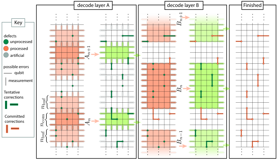
Here we present our main innovation to overcome the backlog problem, which we call parallel window decoding. We illustrate the method in Fig. 3. As in Fig. 2, our illustration is for a repetition code example, naturally extending to a surface code, with further extensions discussed in Section I.5.
Parallel window decoding proceeds in two layers. First, we process a number of non-overlapping windows in decode layer A concurrently. As opposed to the sliding window approach, there are potentially unprocessed defects preceding the rounds in an A window. We thus need to include a buffer region both preceding and following the commit regions. Additionally, we set both time boundaries to be rough, connecting the first and last round of defects to the boundary node. We set , giving a total of per window for some constant . Using the same reasoning as with the sliding window we set . Note that in Fig. 3 we use to keep the illustration compact.
Having committed to corrections in adjacent windows and computed the resulting artificial defects, in layer B we fill in the corrections in the rounds between the neighbouring A commit regions. For convenience, we separate A windows by rounds, so that B windows also have rounds. As the corrections preceding and succeeding the rounds in B windows have been resolved in layer A, the B windows have smooth time boundaries and do not require buffers.
Crucially, if the size of windows and the commit region in layer A are chosen appropriately, we expect no significant drop in logical fidelity compared to the global decoder. As with sliding windows, this is because each error chain of length is guaranteed to be fully captured within one of the windows. In Fig. 4a we verify this by simulating the decoding process. We find that the logical error rates of rotated planar codes using the global MWPM and parallel window MWPM are within the numerical error of each other across a range of code sizes and number of measurement rounds. The same holds for UF-based decoders with data presented in the Appendix C.
This approach is highly parallelizable: as soon as the last round of window has been measured, the data can be given to a worker process to decode it. However, as the window requires the artificial defects generated by windows and adjacent to it (see Fig. 3), it can only start once both processes have completed. In the Appendix D, we sketch a schematic defining how the data pipelining could be implemented in an online parallel window decoder to achieve a high utilization of available decoding cores.
Assuming no parallelization overhead, the syndrome throughput will scale linearly with the number of parallel processes . In this case, rounds are committed to in layer A, and in layer B. Each round takes to acquire and the two layers of decoding take . To avoid the backlog problem, we need the acquisition time to be greater than the decoding time:
| (1) |
Therefore, the number of processes needs to be at least:
| (2) |
In practice, the overhead of data communication among worker processes needs to be considered. In the parallel window algorithm, each process only needs to receive defect data before it is started, and return the artificial defects and the overall effect of the committed correction on the logical operators (see Appendix D). Thus, we expect the data communication overhead to be negligible compared to the window decoding time. Indeed, in Fig. 4b we demonstrate this by simulating parallel window decoding in Python using MWPM as the inner decoder, showing how using leads to greater than an order-of-magnitude increase in decoding speed. Some sub-linearity can be seen due to parallelization overheads in software, particularly for low-distance codes where the decoding problem is relatively simple. In the Appendix C, we repeat these simulations using UF decoder where the overhead is more noticeable due to faster decoding of individual windows. However, hardware decoders such as FPGA (Field Programmable Gate Array) and ASIC (Application-Specific Integrated Circuit) are more suited to parallel data processing, allowing a large number of processes without being bottle-necked by the communication overheads (discussed further in Appendix D). Lastly, even with some sub-linearity, the backlog can be averted provided as we really only need that arbitrary decoding speed is achieved with polynomial number of processors.
I.4 Resulting resource overheads
While we can achieve almost arbitrarily high syndrome processing rates, there is still an inherent latency determined by the time to decode each window . If is large compared to the physical QEC round time , we may slow down the logical clock of the quantum computer to compensate for this latency. This slowdown is achieved simply by extending the delay time as shown in Fig. 1. If we pick as described in Eq. 2, at every instance a block of rounds are being decoded at once. The last round for which the full syndrome history has been decoded is therefore going to be rounds behind the most recently measured syndrome data. Therefore, we can set the response time after each -gate (as defined in Fig. 1) to
| (3) |
However, combining Eq. 2 and Eq. 3 the total response time is . That is, for an algorithm with layers of gates, the total response time is . This is in stark contrast to the exponential in response time observed by Terhal Terhal 2015. Furthermore, using an efficient decoder for each window, the average window decode time scales polynomially with code size , so for some constant . Since code size is poly-logarithmic in algorithm depth and width , for some constant . The response time per layer of -gates is a poly-logarithmic factor so . Strictly speaking, this additional overhead increases the decoding volume by a logarithmic factor, but overall still gives a poly-logarithmic complexity.
We define logical clock time as how long it takes to execute one logical non-Clifford gate. Using lattice surgery to perform -teleportation, and assuming no bias between measurement and physical errors, takes time for lattice surgery and response time. This gives a logical clock time of . Alternatively, this time overhead can be converted into a qubit overhead by moving Clifford corrections into an auxiliary portion of the quantum computer Fowler 2012, for example using auto-corrected -gate teleportation Litinski 2019; Gidney and Fowler 2019. In algorithm resource analysis, a common assumption is that gates are performed sequentially Litinski 2019; Berry et al. 2019; Kivlichan et al. 2020; Campbell 2021; Chamberland and Campbell 2022a; Lee et al. 2021; von Burg et al. 2021; Blunt et al. 2022; Chamberland et al. 2022b as then only a few magic-state factories are needed to keep pace. Auto-correction gadgets enable us to perform the next -gate before the response time has elapsed. The price is that an auxiliary logical qubit must instead be preserved for time , after which it is measured in a Pauli basis depending on the outcome of the decoding problem. Therefore, instead of a time overhead we can add auxiliary logical qubits. If we have an algorithm with 100 logical qubits and , then: without auto-correction we incur a time cost; and with auto-correction we instead require 9 auxiliary logicals qubits and so a qubit cost. Under these common algorithm resource assumptions, we find seemingly large time overheads from parallel window decoding can be exchanged for modest qubit overheads. Indeed, the auto-correction strategies trade time for space resource, but the overall space-time volume is preferable under these resource estimation assumptions ( instead of ). Note that the additional space-time volume required for magic state distillation will depend only on the number of magic states produced and not on whether we use auto-corrected teleportation.
I.5 Extensions
Error mechanisms (e.g. errors in the bulk of the surface code) sometimes trigger more than a pair of defects, but reasonable heuristics can often be used to approximately decorrelate these errors to produce a graphical decoding problem. This decorrelation works well for the surface code. However, many codes cannot be decorrelated and require a non-matching decoder. Even when decorrelation approximations are possible, logical fidelities can be improved by using a non-matching decoder that accounts for this correlation information Darmawan and Poulin 2017; Panteleev and Kalachev 2021; Roffe et al. 2020; Higgott et al. 2022. Extensions of parallel window decoding to non-matching inner decoders are outlined in Appendix B.
By judicious choice of window shapes and boundaries, one could consider 3D-shaped windows that divide the decoding problem in both space and time directions. Similarly, we can construct 3D-shaped windows for parallel execution with only a constant number of layers. When slicing in the time direction we only needed 2 layers of windows, but when constraining window size in dimensions a layer construction is possible, with the minimum number of layers being determined by the colorability of some tiling (see Appendix A for details). When performing computation by lattice surgery, during merge operations the code temporally has an extended size Horsman et al. 2012; Litinski 2019; Chamberland and Campbell 2022a; Chamberland and Campbell 2022b, and windowing in the spatial direction will become necessary to prevent the window decode time from significantly increasing. One may also wish to spatially window for a single logical qubit with windows smaller than the code distance since the decoder running time reduces with window size, and therefore the logical clock time may decrease (alternatively auto-correction qubit overhead may reduce). But there are subtle tradeoffs. Firstly, for windows of size in either the space or time direction, there may be adversarial failure mechanisms of weight that are no longer correctly decoded. One may speculate that this reduces the effective code distance to . However, in practice, percolation theory arguments Fawzi et al. 2018 show that for a distance code, the largest error clusters are typically of size . This leaves open the possibility that windows of size will suffice and be of practical value for stochastic (even if not adversarial) noise, though substantial further investigation is required. We remark that this discussion assumes that measurement errors (that create vertical error chains) have a comparable probability as physical Pauli errors. If there is a large measurement error bias, then we must appropriately scale the duration of lattice surgery operations and the vertical extent of our windows.
II Conclusions
Parallel window decoding avoids the exponential backlog growth that is unavoidable (for large enough computations) with sliding window decoders. For many leading hardware platforms, such as superconducting devices, syndrome backlog can be a severe practical obstacle, even for modest code sizes. In recent superconducting experiments a QEC round was performed every 1.1s by Krinner et al. Krinner et al. 2021 and every ns by the Google Quantum AI team Acharya et al. 2022. Our results are applicable to all hardware platforms, but the speed of superconducting quantum computers means these are amongst the most challenging systems for real-time decoding. Indeed, both aforementioned teams instead performed offline decoding, omitting a crucial aspect of scalable error correction.
To meet this challenge, improving the speed of decoders is currently an area of intense research. For example, LILLIPUT Das et al. 2021 is a recently proposed fast online sliding window decoder, implemented as an FPGA-based look-up table. For surface codes, the authors reported that a round of syndrome data could be processed every ns, fast enough even for superconducting qubits. However, the memory requirements of lookup tables scale exponentially in qubit number, making this decoder impractical for all but the smallest code sizes. The UF decoder scales favourably, and modelling of it on a dedicated microarchitecture Das et al. 2020 suggested it would be fast enough for distance 11 surface codes. However, the authors acknowledged “further study is necessary to confirm the validity of our model in a real device”. Riverlane has recently released performance data, showing that real-time FPGA decoding should be possible on superconducting hardware with up-to distance 9 codes Riverlane Team 2022. There have been other approaches to accelerating decoders. A parallelized version of minimum weight perfect matching (MWPM) has been proposed Fowler 2015 but never implemented and its performance is unclear. Adding a predecoding stage has also been identified as a way to further accelerate decoding and potentially boost logical fidelity Anwar et al. 2014; Ueno et al. 2021; Meinerz et al. 2022; Chamberland et al. 2022a; Paler and Fowler 2022; Ueno et al. 2022, but this has not been tested in an online setting. As such, even for modest code distance such as , it is unclear whether conventional decoding approaches will be fast enough.
On the other hand, a parallel window decoder, as introduced here can achieve almost arbitrarily high decoding speed given enough classical resources and some (polynomially scaling) quantum resource overheads. Therefore, this approach resolves both fundamental scalability issues and practical obstacles for hardware with rapid QEC cycle times.
III Methods
All simulations were performed on an AMD EPYC 7742 processor. We used the PyMatching package Higgott 2021 to perform MWPM. For UF we used a custom Python implementation of the algorithm described in Ref. Delfosse and Nickerson 2021.
In all experiments, phenomenological Pauli noise with physical error rate was used, meaning that there is a probability for a data error on every qubit at each round. Further, every syndrome measurement had an error with probability .
To compute the timing for Fig. 4b and additional results in the Appendix C, we perform the decoding on rounds to ensure a full two cycles of parallel decoding, averaging over 5000 repetitions. We assume initialisation and readout in the Z basis, meaning that the initial and final rounds of defects are smooth. Moreover, in parallel window decoding, we take the first round to always “belong” to layer A, and the first rounds of the first window are committed to. The last round belongs to a layer B if the total number of rounds satisfies , in which case the decoding is performed normally with the last B window potentially being of reduced size. Otherwise, the last window belongs to layer A and the commit region of the last window is from the bottom of the regular commit region to the last round.
Acknowledgements.
This project made use of code co-developed with Adam Richardson and Joonas Majaniemi. We thank Kauser Johar for useful discussions. We thank Steve Brierley and Jake Taylor for encouraging this research and related discussions.
Appendix A Parallel window decoding in time and space
Our main argument has centered around how to perform parallel window decoding over windows defined by time intervals. However, as motivated in the main text, we also may want to parallelize with respect to spatial directions. This is required to support long range lattice surgery operations Horsman et al. 2012; Fowler and Gidney 2018; Litinski 2019; Chamberland and Campbell 2022b; Chamberland and Campbell 2022a, and may also be desirable within single patches. Here we outline how this works, with a guiding example given in Fig. 5.
First, given some space (e.g. a decoding graph or hypergraph) we divide the space up into non-overlapping commit regions. We regard each vertex in the decoding problem as having a space-time coordinate in (with for the surface code). Each edge in the decoding graph is assigned a space-time coordinate corresponding to the mid-point between the vertices it connects. For edges connecting to the boundary, we can just equate the non-boundary vertex coordinate with the edge coordinate. Then for any space-time region, we can associate a set of vertices and edges residing within this region. Assuming a topological code that has local stabilizers, then will always be a maximum distance between any pair of vertices connected by an edge.
Therefore, to find a valid ordering of layers, it suffices to solve a colouring problem. That is, we define collections of commit regions and seek to assign them colours, such that (i) no two regions of the same colour are adjacent; (ii) length scales are set so that regions of the same colour are always separated by distance . Given such a colouring, we can map colours to decoding layers, for example , and . Any permutation of layers remains a valid choice.
We can regard commit regions and of Fig. 3 as representing a 2-colouring of a 2D space. This is extended to 3D (and thereby the surface code decoding problem) by extruding into a 3rd dimension. Fig. 5-i shows a hexagonal 3-colouring of a 2D space, and Fig. 5-iii shows the extruded 3D version of this tiling. For a dimensional space there exist tilings that can be coloured using colours with each tile of bounded size, which for instance has been proved in the context of colour codes Bombín 2013; Kubica and Beverland 2015. In Fig. 5-iii, we tile a space using only 3 colours, but the regions are unbounded size with respect to depth in the 3rd dimension. If we desire constant size tiles, then a tiling of 3D space could be achieved using 4 colours.
Our examples show the minimum number of colours. Given a limited number of processors , we may choose to use more colours so that for each colour there are no more than regions.
Next, we consider the buffer regions required to provide confidence in the corrections in the commit regions. In Fig. 3, the buffer windows are placed above and below the commit region of layer A. In higher dimensions, the buffer regions must include all possible error locations (edges) within a distance of the commit region. However, previously committed regions must not be included in the construction of buffers. Additionally, we do not want artificial defects pushed into a previously resolved region. Therefore, where a window meets a previously committed region the boundary must be set to smooth (no artificial defects allowed).
For example, Fig. 5-ii shows buffer regions and boundaries for a hexagonal tiling. In layer , the buffer region extends in every direction from the commit region. All the boundaries in are rough. In layer , the buffer extends in all directions except those already resolved in layer . Furthermore, the layer window boundaries are set rough except where they meet the resolved layer commit regions (where they are instead smooth, as illustrated). The final layer will only have smooth boundaries and no buffer regions.
Appendix B Circuit-level variants noise and non-matching inner decoders
Here we outline how our sliding and parallel window methods generalise to circuit-level noise and non-matching decoding problems. In circuit-level noise, we may have a decoding problem that possibly includes so-called hook errors, which can be represented by additional edges that are neither solely horizontal or vertical, but instead diagonal in an otherwise cubic graph.
Non-matching decoding problems arise when we also include the possibility of hyperedges. That is, given an error , the associated hyperedge is a list of all the defects it triggers should the error occur. If this list of defects contains more than 2 elements, we say it is a hyperedge. To extend our method, we simply partition all the hyperedges into sets that we call commit regions. Two commit regions can be of the same colour (and therefore part of the same layer) provided that there is no vertex/defect contained in hyperedges from both sets.
This partitioning can be performed either by defining a distance metric derived from the hypergraph, or by defining space-time regions and with each hyperedge having a space-time co-ordinate based on the mid-point of its associated vertices. Note that for non-topological codes the decoding hypergraph may not be localized in Euclidean space, though repeated syndrome extraction means that there will be a time axis such that hyperedges contain vertices that are contained within a constant range on the time axis.
For buffer regions, we follow the same recipe as in the matching case. The difference between rough and smooth boundaries needs additional care. Wherever we have a rough boundary (extremal hyperedges in a buffer region that are not adjacent to any previously corrected/committed regions), we need to allow for the possibility of creating artificial defects. This can be achieved by connecting every hyperedge on a rough boundary to the boundary vertex.
Appendix C Numerical validation of decoder performance
In the main text, we presented numerical results for parallel window decoding using a MWPM inner decoder. Here we present and discuss some additional numerical results: the performance of sliding window decoders with a MWPM inner decoder; and parallel window decoding with a UF inner decoder.
In Fig. 6a we confirm that the sliding window decoding has a negligible drop in logical fidelity for , when compared to the global MWPM decoder. Furthermore, in Fig. 6b we measure the decoding frequency as a function of code size for square rotated planar codes. As the code size grows, the decoding frequency is expected to reduce as for both MWPM and UF which is consistent with our data. Therefore, using sliding window decoding combined with any of the leading inner decoding algorithms, there will always be a code distance for which . This sets a limit on the distance up to which error correction codes can scale using sliding window decoding.
Next, we discuss parallel window decoding when UF replaces MWPM as the inner decoder. As with MWPM, we see no significant increase of the logical error rate when using parallel window decoding (Fig. 6c), and a roughly linear increase with the number of processes for large codes. However, in the case of smaller codes the decoding problem is relatively easy and we see diminishing returns with increased parallelism as the parallelization overheads in Python start being comparable with the decoding time of individual windows.
Sending data to a worker process, starting the decoding of a window and receiving the resulting data takes a finite amount of time . Therefore, if all parallel processes will never be fully utilized and the processing will be bottle-necked by these overheads. However, in a hardware decoder, we expect to be below 10ns using modern hardware and syndrome compression techniques Das et al. 2020, allowing us to scale to over processes. As separate processes do not need to share data, further parallelization of data communication is possible, allowing for even higher bandwidths.
Appendix D Decoding pipeline
In Fig. 7, we sketch the data-flow of the parallel window decoder with processes that could be implemented in hardware. As the stream of syndrome data is acquired, it is given to the process manager that is in charge of passing the data to the appropriate decoding block. Each decoding block resolves the rounds of defects given to it using a matching decoder of choice, and a given specification of rough time boundaries. Recall that the decode windows are labelled and respectively, where is an integer. In the -th step, () blocks decode windows () which have rough (smooth) time boundaries (see Fig. 3). The exception are the first and the last blocks of computation whose boundaries depend on the initialized state and the basis of measurement.
When the first rounds have been collected, these are sent to block for decoding, together with the bottom boundary-type information. The next rounds are given to block which has to wait for and to finish before starting, followed by rounds for block and continuing until all blocks are running. Once finishes decoding, it sends the artificial defects and unresolved syndromes from the bottom rounds to , and from the top rounds to . The indices are cyclic with period , meaning that , and block is followed by . When the data from and has been received, the block can start decoding. The committed corrections from all blocks are added together, continuously updating the total correction.
References
- Terhal (2015) B. M. Terhal, Quantum error correction for quantum memories, Reviews of Modern Physics 87, 307 (2015).
- Bravyi and Kitaev (2005) S. Bravyi and A. Kitaev, Universal quantum computation with ideal clifford gates and noisy ancillas, Physical Review A 71, 022316 (2005).
- Litinski (2019) D. Litinski, A game of surface codes: Large-scale quantum computing with lattice surgery, Quantum 3, 128 (2019).
- DiVincenzo and Aliferis (2007) D. P. DiVincenzo and P. Aliferis, Effective fault-tolerant quantum computation with slow measurements, Phys. Rev. Lett. 98, 020501 (2007).
- Chamberland et al. (2018) C. Chamberland, P. Iyer, and D. Poulin, Fault-tolerant quantum computing in the Pauli or Clifford frame with slow error diagnostics, Quantum 2, 43 (2018).
- Holmes et al. (2020) A. Holmes, M. R. Jokar, G. Pasandi, Y. Ding, M. Pedram, and F. T. Chong, Nisq+: Boosting quantum computing power by approximating quantum error correction, in 2020 ACM/IEEE 47th Annual International Symposium on Computer Architecture (ISCA) (IEEE, 2020) pp. 556–569.
- Chamberland et al. (2022a) C. Chamberland, L. Goncalves, P. Sivarajah, E. Peterson, and S. Grimberg, Techniques for combining fast local decoders with global decoders under circuit-level noise, arXiv preprint arXiv:2208.01178 (2022a).
- Dennis et al. (2002) E. Dennis, A. Kitaev, A. Landahl, and J. Preskill, Topological quantum memory, Journal of Mathematical Physics 43, 4452 (2002).
- Fowler et al. (2009) A. G. Fowler, A. M. Stephens, and P. Groszkowski, High-threshold universal quantum computation on the surface code, Physical Review A 80, 052312 (2009).
- Higgott (2021) O. Higgott, PyMatching: A python package for decoding quantum codes with minimum-weight perfect matching, arXiv preprint arXiv:2105.13082 (2021).
- Delfosse and Nickerson (2021) N. Delfosse and N. H. Nickerson, Almost-linear time decoding algorithm for topological codes, Quantum 5, 595 (2021).
- Das et al. (2020) P. Das, C. A. Pattison, S. Manne, D. Carmean, K. Svore, M. Qureshi, and N. Delfosse, A scalable decoder micro-architecture for fault-tolerant quantum computing, arXiv preprint arXiv:2001.06598 (2020).
- Huang and Brown (2021) S. Huang and K. R. Brown, Between shor and steane: A unifying construction for measuring error syndromes, Physical Review Letters 127, 090505 (2021).
- Iyengar et al. (2012) A. R. Iyengar, M. Papaleo, P. H. Siegel, J. K. Wolf, A. Vanelli-Coralli, and G. E. Corazza, Windowed decoding of protograph-based LDPC convolutional codes over erasure channels, IEEE Transactions on Information Theory 58, 2303 (2012).
- Tan et al. (2022) X. Tan, F. Zhang, R. Chao, Y. Shi, and J. Chen, Scalable surface code decoders with parallelization in time, arXiv preprint arXiv:2209.09219 (2022).
- Fowler (2012) A. G. Fowler, Time-optimal quantum computation, arXiv preprint arXiv:1210.4626 (2012).
- Gidney and Fowler (2019) C. Gidney and A. G. Fowler, Flexible layout of surface code computations using autoccz states, arXiv preprint arXiv:1905.08916 (2019).
- Berry et al. (2019) D. W. Berry, C. Gidney, M. Motta, J. R. McClean, and R. Babbush, Qubitization of arbitrary basis quantum chemistry leveraging sparsity and low rank factorization, Quantum 3, 208 (2019).
- Kivlichan et al. (2020) I. D. Kivlichan, C. Gidney, D. W. Berry, N. Wiebe, J. McClean, W. Sun, Z. Jiang, N. Rubin, A. Fowler, A. Aspuru-Guzik, et al., Improved fault-tolerant quantum simulation of condensed-phase correlated electrons via trotterization, Quantum 4, 296 (2020).
- Campbell (2021) E. T. Campbell, Early fault-tolerant simulations of the hubbard model, Quantum Science and Technology 7, 015007 (2021).
- Chamberland and Campbell (2022a) C. Chamberland and E. T. Campbell, Universal quantum computing with twist-free and temporally encoded lattice surgery, PRX Quantum 3, 010331 (2022a).
- Lee et al. (2021) J. Lee, D. W. Berry, C. Gidney, W. J. Huggins, J. R. McClean, N. Wiebe, and R. Babbush, Even more efficient quantum computations of chemistry through tensor hypercontraction, PRX Quantum 2, 030305 (2021).
- von Burg et al. (2021) V. von Burg, G. H. Low, T. Häner, D. S. Steiger, M. Reiher, M. Roetteler, and M. Troyer, Quantum computing enhanced computational catalysis, Physical Review Research 3, 033055 (2021).
- Blunt et al. (2022) N. S. Blunt, J. Camps, O. Crawford, R. Izsák, S. Leontica, A. Mirani, A. E. Moylett, S. A. Scivier, C. Sünderhauf, P. Schopf, et al., A perspective on the current state-of-the-art of quantum computing for drug discovery applications, arXiv preprint arXiv:2206.00551 (2022).
- Chamberland et al. (2022b) C. Chamberland, K. Noh, P. Arrangoiz-Arriola, E. T. Campbell, C. T. Hann, J. Iverson, H. Putterman, T. C. Bohdanowicz, S. T. Flammia, A. Keller, et al., Building a fault-tolerant quantum computer using concatenated cat codes, PRX Quantum 3, 010329 (2022b).
- Darmawan and Poulin (2017) A. S. Darmawan and D. Poulin, Tensor-network simulations of the surface code under realistic noise, Physical review letters 119, 040502 (2017).
- Panteleev and Kalachev (2021) P. Panteleev and G. Kalachev, Degenerate quantum LDPC codes with good finite length performance, Quantum 5, 585 (2021).
- Roffe et al. (2020) J. Roffe, D. R. White, S. Burton, and E. Campbell, Decoding across the quantum low-density parity-check code landscape, Physical Review Research 2, 043423 (2020).
- Higgott et al. (2022) O. Higgott, T. C. Bohdanowicz, A. Kubica, S. T. Flammia, and E. T. Campbell, Fragile boundaries of tailored surface codes, arXiv preprint arXiv:2203.04948 (2022).
- Horsman et al. (2012) C. Horsman, A. G. Fowler, S. Devitt, and R. Van Meter, Surface code quantum computing by lattice surgery, New Journal of Physics 14, 123011 (2012).
- Chamberland and Campbell (2022b) C. Chamberland and E. T. Campbell, Circuit-level protocol and analysis for twist-based lattice surgery, Physical Review Research 4, 023090 (2022b).
- Fawzi et al. (2018) O. Fawzi, A. Grospellier, and A. Leverrier, Constant overhead quantum fault-tolerance with quantum expander codes, in 2018 IEEE 59th Annual Symposium on Foundations of Computer Science (FOCS) (IEEE, 2018) pp. 743–754.
- Krinner et al. (2021) S. Krinner, N. Lacroix, A. Remm, A. Di Paolo, E. Genois, C. Leroux, C. Hellings, S. Lazar, F. Swiadek, J. Herrmann, et al., Realizing repeated quantum error correction in a distance-three surface code, arXiv preprint arXiv:2112.03708 (2021).
- Acharya et al. (2022) R. Acharya, I. Aleiner, R. Allen, T. I. Andersen, M. Ansmann, F. Arute, K. Arya, A. Asfaw, J. Atalaya, R. Babbush, et al., Suppressing quantum errors by scaling a surface code logical qubit, arXiv preprint arXiv:2207.06431 (2022).
- Das et al. (2021) P. Das, A. Locharla, and C. Jones, Lilliput: A lightweight low-latency lookup-table based decoder for near-term quantum error correction, arXiv preprint arXiv:2108.06569 (2021).
- Riverlane Team (2022) Riverlane Team, Deltaflow.Decode Technical White Paper (2022).
- Fowler (2015) A. Fowler, Minimum weight perfect matching of fault-tolerant topological quantum error correction in average parallel time, Quantum Information and Computation 15, 145 (2015).
- Anwar et al. (2014) H. Anwar, B. J. Brown, E. T. Campbell, and D. E. Browne, Fast decoders for qudit topological codes, New Journal of Physics 16, 063038 (2014).
- Ueno et al. (2021) Y. Ueno, M. Kondo, M. Tanaka, Y. Suzuki, and Y. Tabuchi, Qecool: On-line quantum error correction with a superconducting decoder for surface code, in 2021 58th ACM/IEEE Design Automation Conference (DAC) (IEEE, 2021) pp. 451–456.
- Meinerz et al. (2022) K. Meinerz, C.-Y. Park, and S. Trebst, Scalable neural decoder for topological surface codes, Physical Review Letters 128, 080505 (2022).
- Paler and Fowler (2022) A. Paler and A. G. Fowler, Pipelined correlated minimum weight perfect matching of the surface code, arXiv preprint arXiv:2205.09828 (2022).
- Ueno et al. (2022) Y. Ueno, M. Kondo, M. Tanaka, Y. Suzuki, and Y. Tabuchi, Neo-qec: Neural network enhanced online superconducting decoder for surface codes, arXiv preprint arXiv:2208.05758 (2022).
- Fowler and Gidney (2018) A. G. Fowler and C. Gidney, Low overhead quantum computation using lattice surgery, arXiv preprint arXiv:1808.06709 (2018).
- Bombín (2013) H. Bombín, An introduction to topological quantum codes, arXiv preprint arXiv:1311.0277 (2013).
- Kubica and Beverland (2015) A. Kubica and M. E. Beverland, Universal transversal gates with color codes: A simplified approach, Phys. Rev. A 91, 032330 (2015).