Causal Fourier Analysis on Directed Acyclic Graphs and Posets
Abstract
We present a novel form of Fourier analysis, and associated signal processing concepts, for signals (or data) indexed by edge-weighted directed acyclic graphs (DAGs). This means that our Fourier basis yields an eigendecomposition of a suitable notion of shift and convolution operators that we define. DAGs are the common model to capture causal relationships between data values and in this case our proposed Fourier analysis relates data with its causes under a linearity assumption that we define. The definition of the Fourier transform requires the transitive closure of the weighted DAG for which several forms are possible depending on the interpretation of the edge weights. Examples include level of influence, distance, or pollution distribution. Our framework is specific to DAGs and leverages, and extends, the classical theory of Moebius inversion from combinatorics. For a prototypical application we consider the reconstruction of signals from samples assuming Fourier-sparsity, i.e., few causes. In particular, we consider DAGs modeling dynamic networks in which edges change over time. We model the spread of an infection on such a DAG obtained from real-world contact tracing data and learn the infection signal from samples.
Index Terms:
Graph signal processing, DAG, partial order, causality, structural equation model, Moebius inversion, Fourier transform, convolution, non-Euclidean, Fourier sparsity, dynamic graph, infection spreading, binary classifierI Introduction
Causality studies which events influence others building on powerful classical theories including Bayesian networks and structural causal models [1, 2]. However, understanding and deriving causality from data continues to be a challenging problem in data science and machine learning [3]. The common index domains for causal data are directed acyclic graphs (DAGs), in which the nodes represent events and the directed edges causal relationships. Motivated by their importance, we propose a novel form of Fourier analysis for signals (or data) on DAGs, including associated signal processing (SP) concepts of shift, convolution, spectrum, frequency response, and others. DAGs are closely related to partially ordered sets (posets), where the partial order determines whether a node is a predecessor of another node. Thus, our SP framework can equivalently be considered for signals on posets.
Our framework is specific for DAGs and fundamentally different from prior graph SP based on Laplacian or adjacency matrix [4, 5], which fails for DAGs due to a collapsing spectrum. The causal nature of our framework is reflected in both shift and associated Fourier transform as will become clear later. Before we state our contribution in greater detail we provide the context of prior work. A more detailed discussion of related work is provided later in Section V.
Graph signal processing. Prior graph SP uses the eigenbasis of adjacency matrix or Laplacian as Fourier basis and to define related concepts [5, 4]. For undirected graphs both exist and are even orthogonal. For directed graphs (digraphs) this is not the case, the more general Jordan normal form is not computable, and thus a proper digraph SP was still considered an open problem in [6, Sec. III.A] despite various applications [7]. Several solutions have been proposed, mostly based on a form of approximation or relaxation of requirements [8, 9, 10, 11, 12, 13].
DAGs constitute a worst case in digraph SP since they are associated with triangular Laplacian or adjacency matrices. In particular the latter have only one eigenvalue zero and thus never an eigenbasis. The lack of a proper form of DAG Fourier analysis prevents the application of SP methods to causal data indexed by DAGs.
Causality. Classical models for causality include Bayesian networks [1], which encode multivariate probability distributions and enable different forms of causal reasoning. Structural causal models (SCMs), also called structural equation models (SEMs) [2], define how variables associated with DAG nodes are computed from parent nodes. Both approaches are probabilistic and model data as random vectors on DAGs, in which the edges represent causal dependencies. Despite powerful theory, learning causality from data is hard with many pitfalls [14, 15, 3]. In particular, causal data typically has a DAG as index domain, but the converse does not hold: if data is given on a DAG, its edges do not generally imply causal relationships due to possible hidden confounding variables, and detecting causality does require additional techniques such as interventions [2]. One important line of work in causal reasoning addresses the problem of learning the DAG from observed data [16, 17].
Our proposed Fourier analysis could bring a novel view point and SP-inspired tools to the analysis of causal data. As a first step, we have tackled a novel variant of DAG learning [18], based on the assumption of sparsity in the Fourier domain.
Contribution. We present a novel form of Fourier analysis, and associated basic SP concepts, for signals (or data) indexed by the nodes of a weighted DAG, extending and completing our preliminary work in [19]. Our framework can be used on any DAG signal, whether the DAG captures causality or not. However, in the causal case, and under assumptions and in a sense that we define, the causes of a signal become its spectrum on the DAG in our Fourier analysis. Further, our framework can be related to the special class of linear SEMs, providing a novel Fourier-perspective.
In contrast to prior graph SP, our work leverages the partial order structure defined by a DAG, which also makes it specific to the acyclic case. The weighted DAG describes how the signal value at a node is determined (or caused in the causal case) by its parent nodes. But, by transitivity, this means that the value is determined by all predecessors. We assume this relation to be linear and thus it is obtained by a suitable form of weighted transitive closure of the DAG [20], whose form depends on the meaning of the weights, such as distance, level of influence, or fraction of propagation. Viewed as a matrix, the transitive closure determines the Fourier basis relating a signal to its causes, which become its spectrum. We define an associated notion of shift that operates in the frequency domain by removing causes, and show that the spectrum is partially ordered isomorphic to the DAG.
Our prototypical experiments consider the reconstruction of DAG signals from samples under the assumption of sparsity in the Fourier domain. We show a synthetic experiment as proof of concept. Then we consider one possible application domain for our work: dynamic networks whose edges change over time, which can be modeled as DAGs by unrolling the time dimension and connecting subsequent iterations of the graphs accordingly. We model the spread of a disease on such a DAG, derived from real-world contact tracing data. Then we learn the infection signal from samples. Our causal Fourier basis yields superior results when compared to prior graph Fourier bases, which require dropping the directionality of the edges.
II DAGs and Posets
We explain the necessary background on directed acyclic graphs (DAGs), partially ordered sets (posets), and their close relationship. Sets and graphs are denoted with calligraphic letters, matrices in upper case, vectors in bold lower case, and scalars in lower case.
DAGs. A directed graph (digraph) consists of a finite set of nodes and a set of directed edges: . is acyclic, and thus a DAG, if it contains no cycles. Since is acyclic, we can sort topologically, which means implies that comes after . We consider weighted DAGs , in which each edge is assigned a nonzero (not necessarily positive) weight . These are collected in the matrix
| (1) |
The topological sort makes lower triangular with zeros on the diagonal. If all weights are , is just the adjacency matrix.
Posets. A partially ordered set (poset) [21] is a finite set with a partial order, i.e., a binary relation that satisfies for all
- 1.
(reflexivity),
- 2.
and implies (antisymmetry),
- 3.
and implies (transitivity).
We write if but . An element covers if and there is no in-between, i.e., with [22].
Relation between DAGs and Posets. Every DAG induces a unique partial order on , defined as if is a predecessor of , i.e., if there is a path from to .
Conversely, for a given poset there are several DAGs that induce it, but two are special and unique. One is the reachability graph with . This DAG is transitively closed, i.e., whenever there is a path from to there is also an edge . We mark this property with an overline. The other unique DAG inducing is the cover graph with . This graph is transitively reduced, i.e., the DAG with the fewest number of edges inducing . It contains no edge if there is another path from to in .
Example. In Fig. 1 we show an example of a DAG together with its transitive reduction and its transitive closure. All three DAGs induce the same poset.
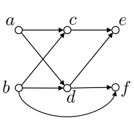
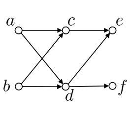
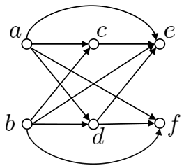
In summary, every DAG uniquely defines a poset, whereas a poset can be represented by several DAGs. These however, have the same transitive reduction or transitive closure. Next we will build our signal model, which will require the computation of a transitive closure that also takes the weights into account.
III Signal Model and Weighted Transitive Closures
We define the signal model that underlies our proposed Fourier analysis and the associated related SP concepts that we derive in the following section. The key aspect here is that the model, and thus the associated Fourier analysis, is not uniquely determined by the given weighted DAG but also requires a choice of weighted transitive closure that captures long-distance influences in , i.e., for where is not a parent of . We motivate the need for transitive closure and discuss relevant choices that depend on the meaning of the edge weights in , leveraging the theory in [20].
III-A Basic signal model
We assume a given weighted DAG with induced partial order on , . We consider signals on as column vectors of the form
where the order of the is determined by the chosen topological sort of .
We call each an event and say that an event is a cause of the event if . Further, we assume that every event is associated with an unknown contribution (or input) to the DAG and that the (measured) signal value at is given by the weighted sum of the over all causes :
| (2) |
By (slight) abuse of notation we also say that , for , is a cause of .
Intuitively, the weights in (2) determine the influence of the causes of on . Collecting the in a matrix yields the equivalent form
| (3) |
where is lower triangular and its nonzero entries correspond to edges in the reachability graph associated with (e.g., Fig. 1(c)).
Example and motivation. As a simple, high level example (that we also used in the follow-up work [18]), consider a river network, which is a DAG since water only flows downstream. The nodes correspond to a set of fixed locations (e.g., cities). We assume that each node inserts an unknown amount of pollution, and that is the pollution measured at , accumulated from all predecessors. The weight in could quantify what fraction of pollution at reaches a direct successor .
The measured pollution is determined by the of all causes of (not just the parents of ) and in (2) would capture their relative contribution. As we will explain below, is obtained from through a weighted transitive closure. Its exact form will depend on the meaning of the edge weights .
On the use of the term “cause”. We use the term cause since we believe it helps with understanding our model. However, as already mentioned in the introduction, we want to stress again that (2) does not imply causality but could just express a linear relation, excluding hidden, confounding variables. Thus, strictly speaking, the term “cause” for the is not correct in this case. We still use it to emphasize that if (2) is a causal relationship, it does relate signal values and causes, and since it helps with understanding the different forms of transitive closure discussed next. In any event, our Fourier analysis and entire framework is applicable to any signal on any DAG.
III-B Weighted Transitive Closure
The DAG and its edge weights captures how each node is influenced by its parents. But, as we also saw in the river network example, if is a parent of and is a parent of , then, by transitivity, also will influence . The associated weight will depend on the meaning of the edge weights in . We build on the theory in [20].
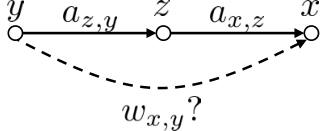
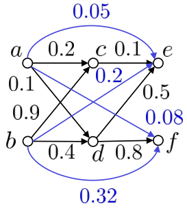
As a simple example, consider the transitive closure of the very small DAG in Fig. 2, i.e., the computation of . In the river network example, fractions would multiply, i.e., . If the weights denoted distance, , if they denoted throughput, , and so on.
Next, we consider these and other choices that can be used to define for all , given . This is equivalent to computing a weighted transitive closure of and setting for . is the reachability graph defining the same partial order as . Then we will define to obtain the entire matrix in (3).
Boolean weights: Standard transitive closure. If is the adjacency matrix, i.e., binary with all nonzero weights , one obvious choice is to give all edges in the transitive closure the weight as well, i.e., set as the adjacency matrix of .
Pollution. As in the example of the last section, the weights in could encode what fraction of a potential pollutant inserted at a node arrives at a direct successor . Thus the weights are in and, for each node, the sum of the weights of outgoing edges should be . The transitive closure would then contain the same information, but now for each pair of nodes connected by a path. The fractions multiply along paths and have to be summed over all paths to obtain the result.
In this case there is a known formula [20], which uses that :11 1 The equation follows from the telescoping sum .
| (4) |
Reliability/influence. The weights in could encode reliability or influence factors in , where means 100% reliability of the edge or influence of on and means none. Along paths, these influences multiply and could encode the most reliable/influential path from to .
Shortest path. The weights in could encode distances in between nodes. In this case, the weights in could be defined as the shortest path from to in . Since one would assume causes that are farther from in to have less influence, one could consider derivatives of a path length such as or . The latter choice effectively converts distances to influences in the sense discussed right above.
Maximal capacity. The weights in could encode capacity or throughput of edges. The capacity of a path is determined by the minimal capacity among its edges and could encode the maximal capacity path between and .
| Meaning of edge weight in closure | |||||
|---|---|---|---|---|---|
| is reachable from , i.e., | |||||
| Fraction of pollution from reaching | |||||
| Strongest influence/most reliable path from to | |||||
| Shortest path length from to | |||||
| Largest capacity path from to |
Computation. Various algorithms are available to compute transitive closures and their associated weights. The special cases that we just presented can be solved with one generic algorithm, instantiated in different ways [23]. We show it in its simplest form in Fig. 3; an optimized version can be found in [23]. The algorithm is initialized with the weight matrix on which it performs iterations for a total runtime of . It is generic in the choice of addition and multiplication used, which must satisfy a semiring property22 2 See [23, Definition 2.1]. In particular, is commutative, and are associative, have an identity element, and satisfy the distributivity law..
Table I shows several choices of semirings and the associated result of the algorithm. Fig. 4 provides intuition: determines how consecutive weights are combined (e.g., product for reliability, sum for path length), and how weights of alternative paths are combined (e.g., sum for pollution, min for shortest path length). If these two operations satisfy the semiring property, then the algorithm in Fig. 3 works.


Note that with and also the definition of (identity element for addition) and (identity element for multiplication) changes as shown in the table. E.g., for shortest path, since . Thus, in the algorithm, zeros in have to be replaced with upon initialization.
For shortest path, the algorithm is equivalent to the classical Floyd-Warshall algorithm [24].
Other choices of weighted transitive closure may require other algorithms. E.g., overall capacity between two nodes requires max-flow algorithms [25]. The related structural equation models (discussed later in Section V) use the pollution model but without constraints on the weights.
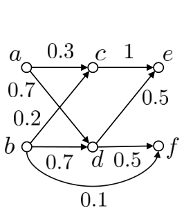
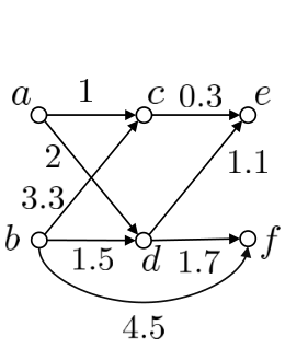
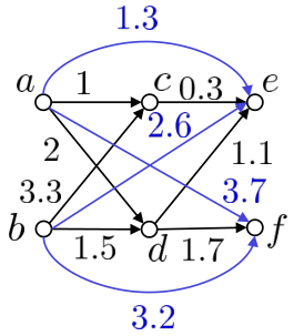
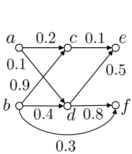
Examples. Fig. 5 shows a few examples of transitive closures, using the DAG from Fig. 1(a) as starting point. Note that the transitive closure may overwrite weights in . E.g., the bottom edge in Fig. 5(e) has weight , but after closure, the shortest path from to has length .



III-C Reflexive closure
Finally, we need to define in (2), which accounts for reflexivity in the partial order, i.e., the fact that is a cause of . Our model requires , since later we want the triangular matrix in (3) to be invertible. In this paper we focus on the choice . For the special case of pollution, we obtain a closed form using (4):
| (5) |
In other cases, takes a different forms as computed by the algorithm in Fig. algo:ModifiedFloydWarshall.
In three of the fives cases in Table I the choice of coincides with (fraction of pollution or influence of a node on itself is ), but poses a problem for the others. For shortest paths this suggests, for example, and as we also do later, converting path length to exponential decay , which makes it a particular influence model, effectively converting the operations to . For capacity one could choose for capacity .
Summary. Both and are lower triangular matrices with zeros on the diagonal and thus as the only eigenvalue. is lower triangular with ones on the diagonal and thus of full rank, i.e., its columns form a basis, which, in fact, will become our proposed Fourier basis as explained in the next section.
IV Causal Fourier Analysis on DAGs
Given a weighted DAG with associated partial order , we assume we have decided on a suitable transitive/reflective closure of as explained in Section III. We restate our signal model, which assumes that a signal on is a linear combination of unknown causes associated with the nodes:
| (6) |
In this section we will build on this equation to develop a linear SP framework for signals on DAGs. In short, we will argue that c can be interpreted as a form of spectrum of s, with as associated Fourier transform. We do so following the general theory in [26, 27]: we define a suitable notion of shift and convolution for which the columns of form a joint eigenbasis. Our derivations leverage the classical theory of Moebius inversion from combinatorics [22], which is concerned with equations on posets of the form in (6). We start by inverting (6).
IV-A Calculating Causes: Moebius Inversion
In the case of the standard Boolean transitive closure, i.e., trivial nonzero weights , the calculation of c from s is provided by the classical Moebius inversion from [22]. The extension to arbitrary transitive closures and weights needed here is straightforward and provides a formula for .
Theorem 1.
| (7) |
Here is the weighted Moebius function, recursively defined as
We provide a proof in the appendix. is lower triangular with ones on the diagonal since the same holds for .
IV-B From Shift to Fourier Transform
The following definition of the shift operation is a key contribution of this paper. At first glance it is non-obvious but is the one that generalizes our prior SP framework on lattices [28] to arbitrary posets and weighted DAGs. As we will see, it can be viewed as a form of causal delay, takes an intuitive form in the case of Boolean weights, makes the columns of the associated Fourier basis, and thus the causes become the spectrum. Once the shifts are defined, the derivation of the remaining basic SP concepts is straightforward [26].
Causal shifts. We first provide the formal shift definition and then interpret it. For every we define a linear shift operator, given by a matrix , on s:
| (8) |
In words, comparing to (6), the result is the signal with all causes removed, which are not common causes of and .
But to obtain a proper representation of this linear mapping we need to express the right-hand side of (8) as linear combination of signal values, not causes. We do this by replacing in (8) using the inversion formula in (7):
| (9) |
Inspecting (9) shows that is a linear combination of signal values with and (i.e., “earlier” in the DAG order), as visualized in Fig. 6(a). Thus we consider it as a form of “causal delay.”
We consider special cases to motivate the definition. Assume that and have a unique greatest lower bound in denoted with , i.e.: for all with we have (which is the case if the poset is even a lattice [22]). In this case, (9) simplifies to
| (10) |
i.e., it is linear combination of signal values of nodes . This situation is visualized in Fig. 6(b) with .
Assume in addition that is the Boolean transitive closure of an unweighted DAG given by , which is the situation in the prior work [28]. Then, now by specializing (8),
| (11) |
i.e., the causal delay takes its most beautiful form (in Fig. 6(c) the result is ) and can be conceptually compared to the classical shift of a discrete-time signal by , which maps to .


Equation (8) shows that all shift matrices , , commute since they only affect the range of summation, and that they are idempotent, i.e., . Further, (9) shows that signal values are shifted to linear combination of predecessors; thus the are lower triangular and in general not invertible.
Filters and convolution. The shifts generate the algebra (ring and vector space) of filters [26]. Since the shifts commute, a filter is a polynomial in the shifts. Since , the most general filter, represented as matrix, is for . Thus, for , the associated convolution takes the form
| (12) |
As polynomials in the shifts, filters are shift-invariant, i.e., for all .
Fourier basis and transform. The Fourier basis consists of the joint eigenvectors of all and thus all filters. Its derivation is simple due the definition of . Let . Equation (8) shows that shifting s by performs a pointwise multiplication on c. Formally, we can write (8) as
| (13) |
where is the indicator function
| (14) |
In words, removes the causes of any signals that are not also causes of .
Replacing in (13) shows that for all we have , and thus
Since has full rank, the columns are the desired Fourier basis:
Theorem 2 (Fourier basis).
The columns of from a simultaneous eigenbasis of all shifts and filters, i.e., the Fourier basis vectors are
| (15) |
The associated Fourier transform is obtained by inversion:
Theorem 3 (Fourier transform).
The Fourier transform associated with the above Fourier basis is given by
with Fourier transform matrix (Theorem 1)
Frequency response and convolution theorem. Equation (13) shows that the frequency response of a shift is the diagonal of , i.e., by (13). Thus, for a general filter h corresponding to the matrix , it is the diagonal of .
Denoting the frequency response of h as we obtain
| (16) |
and the associated convolution theorem:
| (17) |
where denotes pointwise multiplication. In words, convolution (filtering) in the signal domain is equivalent to pointwise multiplication (by the frequency response of the filter) in the frequency domain. A few things are worth noting.
The Fourier transform and frequency response are computed differently, which is also the case in graph signal processing and generally due to the different roles of signal and filter space [26].
The frequency response is computed only based on the partial order defined by the DAG, i.e., independent of the weights and the chosen transitive closure.
Computing from h is a linear transform with an lower triangular transform matrix with ones on the diagonal. As such it is invertible, which means every frequency response can be achieved with a suitable filter. In particular, the trivial filter with , , i.e., is a suitable linear combination of the . The inversion of the frequency response can be done with the dual version of Theorem 1, i.e., in which is replaced with .
Fast algorithms. Explicitly computing the Fourier transform matrix by inverting requires operations. In practice, since the matrix and its inverse are lower triangular, the spectrum of a signal s can be computed without explicitly constructing using a triangular solve of
| (18) |
using operations.
In the case of unweighted (i.e., Boolean weights) DAGs the Fourier transform and its inverse can be computed using time and memory, where is the width of the DAG, i.e., the longest antichain or maximal number of mutually non-comparable elements of the DAG [29]. For small this enables the computation for DAGs up to millions of nodes.
Total variation and frequency ordering. We complete our framework by a suitable definition of frequency ordering. Here we follow the high-level idea used for graphs by [5], which relates frequency ordering to the shift via total variation (TV). Here, however, we have multiple shifts and thus we consider TV separately for each shift, as common for images (with two shifts: horizontal and vertical translation) and as was done previously in [28] for meet/join lattices, which thus we generalize here.
Definition 1.
Let s be a signal on . We define the variation w.r.t. a shift by as . The total variation of s is then the vector
| (19) |
and the sum total variation is the number
| (20) |
We next show that the Fourier basis, and thus the spectrum, is partially ordered in a way isomorphic to the partial order induced by , with low frequencies corresponding to the early nodes in the DAG, i.e., the smallest ones in the induced partial order.
Theorem 4.
We normalize to . Then
| (21) |
and thus
| (22) |
The poset of total variations w.r.t componentwise comparison is isomorphic to the (unweighted) poset induced by , i.e., if and only if . STV provides a topological sort of the frequencies.
We provide a proof in the appendix. Note that the frequency ordering only depends on the partial order induced by the DAG and not by the chosen weighted transitive closure. Also, the frequency ordering is independent of the choice of the two norms occurring in Theorem 4.
Next we provide a numerical example for the concepts introduced and then we conclude this section by a discussion of salient aspects of our framework.
IV-C Small Example
For a small example we consider the DAG in Fig. 5(c), which is given by
Further, we assume the pollution model, i.e., the transitive closure of is given by Fig. 5(d), which, including the reflexive closure, yields the matrix
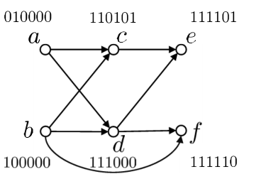
Fourier basis and frequency ordering. The columns of constitute the Fourier basis of the DAG. The first two have the lowest frequency w.r.t. the total variation in Definition 1. For example . All are shown in Fig. 7. Note, for example, that but .
Fourier transform. The inverse Fourier transform connecting signal and causes (spectrum) is given by . Thus the Fourier transform becomes . The Fourier transform matrix is given by :
| (23) |
Shifts. As an example, the shift is given by the matrix
| (24) |
For example,
| (25) |
which is a linear combination of signal values on common predecessors of and in .
Low-pass filter. In classical discrete-time SP, a basic low-pass filter is constructed by averaging a signal with its shifted version . Analogously, we construct a low-pass filter by summing the trivial shift and all shifts by , , and normalize by the largest eigenvalue: .
In our example, the trivial filter can be written as and thus with coordinate vector . In matrix form it is
| (26) |
The frequency response of this filter is which shows that indeed higher frequencies (associated with later nodes in the DAG) are attenuated (the highest two by ), while, in this case, the lowest two are maintained.
IV-D Relation to structural equation models
Structural equation models (SEMs), also called structural causal models (SCMs), are an important tool for analyzing causal data [2], modeled as a DAG of causally dependent random variables that satisfy functional relationships. For the special class of linear SEMs (e.g. [30], which uses them to learn DAGs from data), this relationship is linear.
Assuming, as before, a weighted DAG with nodes, a linear SEM is defined as
| (27) |
where is a random vector and a (usually i.i.d.) random noise vector, not necessarily Gaussian. Using (5) we can write (27) as
| (28) |
if we choose the -transitive closure associated with the pollution model (but now without restriction on the weights) to obtain from . In words, the noise chosen to sample the linear SEM is then, in our sense, the spectrum of the obtained signal.
Conversely, assume a weighted DAG with nodes and an arbitrarily chosen weighted transitive closure (e.g., from Table I), which defines a notion of spectrum in the sense of this paper. Let be the DAG associated with . Then the linear SEM is such that the noise chosen to sample is the spectrum of the obtained signal.
The latter allows the interpretation of any weighted transitive closure in the context of linear SEMs.
V Discussion and Related Work
We discuss related work and some of the salient aspects of our causal SP framework for DAGs.
Comparison to graph SP. Graph SP [6] is concerned with signals indexed by the nodes of a graph and generalizes classical SP concepts by choosing adjacency matrix or Laplacian, or variants thereof as shift (or variation) operator [5, 4], which is known to be the defining concept of any linear SP framework [26]. For undirected graphs, the eigendecomposition of the shift exists and yields an orthogonal Fourier transform. Other SP concepts and techniques take meaningful forms [6]. For directed graphs (digraphs) a proper generalization was still considered an open problem in [6, Sec. III.A], since an eigendecomposition does not exist in general and the more general Jordan normal form is not computable. DAGs constitute, in a sense, a worst case among digraphs since the adjacency shift has only one eigenvalue zero.
Several solutions have been proposed for digraphs. An overview including applications of digraph signal processing can be found in [7]. One approach computes a Fourier basis that minimizes the sum of directed variations [8], or evenly spreads them [9, 10]. Others include changing the shift to the Hermitian Laplacian [11], using an approximation based on the Schur decomposition [12], or adding generalized boundary conditions, i.e., additional edges to the digraph [13].
All these are fundamentally different from our approach which is applicable only to acyclic digraphs and based on a very different notion of shift and Fourier basis. The fundamental difference is best captured in the shift definition: graph shifts capture the neighbor structure, whereas our causal shifts capture the partial order structure provided by DAGs, directly manipulating causes, i.e., values of predecessors inserted to the DAG. As a result, all derived concepts differ substantially. In particular, in our framework DAGs first need to be transitively closed (and their are choices) and the exclusive dependency on predecessors motivated by causality makes shifts and Fourier transform triangular.
Our work can equivalently be interpreted as Fourier analysis for signals on weighted posets, i.e., with a weight assigned to each pair with .
Comparison to lattice SP. Our work substantially generalizes SP on meet/join lattices [31, 28, 32], which, in turn, generalizes SP with set functions from [33, 34]. These lattices are a special class of posets or DAGs, in which each two elements have a unique greatest lower bound, which yields the concise representation of the shift in (10). This paper drops this condition, which makes it applicable to arbitrary posets and thus arbitrary DAGs. Further, and equally important, we allow for non-trivial weights and thus interpretations like distance or influence, which should considerably expand applicability.
Causality and linear SEMs. Most closely related in causality research are linear SEMs as we formally explained in Section IV-D. Typically, in SEMs, linear or not, the causes of a node are the parents because of the form in (27). In this paper we use the term differently, namely for all predecessors of a node motivated by the form in (28).33 3 Thus, in our follow-up work [18] we used the term root causes instead.
Linear SEMs have been studied in [35, 36, 37, 38]. One question is identifiability of the data distribution, which depends on the distribution of in (27). If is i.i.d. Gaussian, linear SEMs can express any -variate distribution with a suitable DAG [38]. In contrast, motivated by our proposed Fourier analysis, our assumption in the linear SEM experiment later in Section VI-A is that is approximately sparse with random support.
An active research area is learning the DAG from data, with various approaches specifically targeting linear SEMs [39, 16, bello2022dagma, 17]. In particular, [16] captures acyclicity as a continuous constraint to obtain a solvable optimization problem. Our work [18] builds on it but changes the data generation from (27) to assume sparsity in the Fourier domain. Thus we believe that our has the potential to bring new, SP-inspired method to the domain of causal data analytics. We also note that the interpretation of different transitive closures as linear SEMs (Section IV-D) appears to be novel.
Multiple shifts. Our framework is shift-invariant and based on multiple basic shifts instead of just one in graph SP. This is not uncommon: e.g., filters on images are composed from independent shifts in and -direction, so also there the spectrum is partially ordered. Fundamentally, it just means that the filter space is a polynomial algebra in multiple variables [26].
SP on non-Euclidean domains. Besides graph SP, other SP frameworks for non-Euclidean domains have been proposed.
One line of work is topological SP [40] based on the Hodge Laplacian, which considers signals defined on simplicial complexes, with values assigned to nodes, edges, or higher-order faces. The framework was generalized to cell complexes in [41, 42].
Hypergraphs generalize graphs by allowing edges with more than two nodes. A topological approach to hypergraph SP similar to above was proposed in [43], whereas [44] uses the adjacency tensor and tensor decomposition to define a notion of spectrum, sampling theory, and filters.
Quiver SP [45] considers directed multigraphs (i.e., multiple directed edges between the same nodes are possible), and develops an SP theory based on the rich representation theory of these structures.
Graphon SP is a continuous extension of SP on undirected graphs, thus enabling sampling among other things [46].
SP on lattices and powersets [28, 34] are direct predecessors of our work as already explained above and our first attempt to go to arbitrary unweighted DAGs was in [19].
Several of the above generalized SP frameworks, and the work in this paper, build on the algebraic signal processing theory, which provides the axioms, insights, and derivation guidelines for any linear SP framework [26, 27] and was used to consider the first shifts beyond standard translation/delay [47, 48, 49].
VI Application: Fourier Sparsity
Our work provides a complete set of basic SP concepts for data on weighted DAGs. Thus, in principle, any SP method that builds on Fourier analysis or filtering can be ported. In this paper we focus on the concept of sparsity in the Fourier domain, which, in the causal setting, has the appealing equivalent interpretation of signals with few causes.
As an example, consider again the river network with measured pollution data from Section III-A. Fourier sparsity means that only few cities polluted in a data set, a reasonable assumption.
There are two problems that one can readily associate with Fourier sparsity:
- •
Reconstructing a DAG signal from samples under the assumption of Fourier sparsity.
- •
Learning the DAG from DAG signals under the assumption of Fourier sparsity.
We proposed a solution, called SparseRC, for the second problem in the follow-up work [18] for the special case of linear SEMs, i.e., the -transitive closure of the pollution model without weight restriction as explained in Section IV-D. The problem had not been considered before. We proved identifiability and showed that SparseRC could successfully learn DAGs up to thousands of nodes under mild assumptions. Further, in the recent CausalBench challenge [50] on learning gene interactions from single cell data, SparseRC was among the three winning teams [51], showing that the assumption of few causes can be relevant in practice.
In this paper we focus on the first problem of reconstructing a signal from samples. First, as a proof of concept, we consider a synthetic problem on randomly generated graphs, again based on a linear SEM. Then, in the following Section VII, we consider a more realistic semi-synthetic experiment at a much larger scale modeling infection spreading on a dynamic network along time. In that experiment the assumption of Fourier-sparsity is intuitive but not explicitly built into the experiment.
VI-A Learning DAG signals from samples
We generate signals on weighted, random DAGs using a corresponding linear SEM under the assumption of approximate Fourier-sparsity with unknown support w.r.t. our associated Fourier basis. Then we reconstruct the signal from samples, using a Lasso-method [52] (i.e., linear regression with a sparsity penalty) that is applicably with any basis. We compare against prior graph Fourier bases obtained by dropping directions in the DAGs.
Random graphs. We construct weighted DAGs with nodes using the Erdős–Rényi model [53], where each edge is created with probability and given a random weight in . To obtain a DAG, we order the nodes randomly and only keep the edges with . We construct DAGs, each one thus with approximately edges.
Signal generation. We generate approximately Fourier-sparse signals on a random DAG using a linear SEM as described in [18]. Namely, the inverse Fourier transform is the -transitive closure (Section IV-D) and the data is generated via
| (29) |
where is the sparse spectrum, i.e., the relevant few causes, is spectral noise, and models the noise in the measurement of . Here the term corresponds to the term in (28). Both and are assumed to be of negligible magnitude compared to . Specifically, we choose to be sparse with only nonzero values at random locations and in the range , and and are i.i.d. zero-mean Gaussian noise with a standard deviation of .
In the river network example, would be the inserted pollution by a city, negligible random pollution inserted by all cities, and the noise in the pollution measurement.
Reconstruction method. We reconstruct the generated signal s from samples at nodes by fitting a Lasso model. That is, we solve a linear regression with an -sparsity penalty:
| (30) |
Here is the -th Fourier basis vector (15), the linear regression approximates the samples as a signal on the DAG, while the -penalty promotes sparsity in the Fourier spectrum. With the minimizing found the obtained reconstructed signal is then
Baselines. As baselines we consider other Fourier bases in (30). Namely, the graph Fourier bases associated with adjacency and Laplacian matrices, for both the DAG and its transitive closure obtained by dropping the directions in the DAG, i.e., the eigenbases of and .
Further, we also consider our binary DAG Fourier basis obtained by setting all nonzero weights in to one and computing the Boolean transitive closure.
Results. Fig. 8 shows the results: the reconstruction error as a function of the fraction of the signal sampled. The shaded areas show the confidence intervals over 100 repetitions.
As expected, given enough samples, the signal can be well reconstructed with the Fourier basis used in its construction. The other bases fail since the signal is not approximately sparse in their Fourier domain. This also applies to our unweighted DAG basis. In other words, the weights and chosen transitive closure matter.
VII Application Example: Dynamic Networks
We present a more realistic example of learning a DAG signal from samples, again under the assumption of Fourier sparsity, i.e., few causes, but this time this sparsity is not present by construction. As signal domain we consider a class of DAGs that is obtained from graphs that change dynamically with time.
Examples of real-world (undirected) graphs include proximity of persons (used, e.g., for contact-tracing of infectious people during a pandemic), peer-to-peer networks between vehicles in traffic, or transactions between traders in a market. However, these graphs are often non-static, e.g., the edges change with time. The work in [54] shows how to encode such a dynamic network as a DAG by assigning the graphs to discrete time steps and connecting subsequent graphs.
We consider such DAGs as one possible application domain of our work and present in this section a prototypical, semi-synthetic example: we use real contact-tracing data to simulate the spread of an infection among individuals along time. Then we try to reconstruct, or learn, this infection signal from samples under the assumption of sparsity in the Fourier domain. We presented a restricted, simplified version of this experiment using unweighted DAGs in [19].
VII-A Infection Spreading on Dynamic DAGs
We explain the construction of DAGs from dynamically changing graphs and the model we use to generate infection signals from contact tracing data.
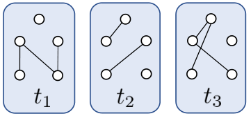
Dynamic networks as DAGs. We consider a dynamic network as a collection of (undirected) graphs where the set of edges changes with time . It can be modeled as a DAG using the idea from [54]. Namely, we make a copy of the node set for each time point, i.e., the new node set is , where is an added, last time point.
Further, we connect nodes with if and always with to form . This construction is illustrated on a small example in Fig. 9.


The Haslemere data set. We consider the data set from [55], which uses real smartphone proximity data to obtain a dynamic network on which the spread of a disease is then modeled and analyzed. Here we aim to learn the associated signal from samples. Concretely, the proximity of participants was measured for three days every 5 minutes between 7am and 11pm using a smartphone app, resulting in time points. Due to our infection model below we remove all edges with distance meters.
Haslemere DAG. With the above construction we turn the Haslemere dynamic network into a DAG . Since later we want to use standard graph SP as benchmark (with directions dropped), which requires an eigendecomposition of the Laplacian or adjacency matrix, we have to restrain the size of . Thus, we sample the contact data only every hour, resulting in time points leading to a DAG with nodes and edges.
Weights. At each time point the edges of the graphs are weighted by the distance of the participants. We convert the distances into influences as explained in Section III-B to ensure fading with large distances in space and, through the transitive closure, in time. Concretely, DAG edges of the form obtain weight 1, and edges of the form obtain weight , where is the distance at time . The transitive closure is then computed using Algorithm 3.
Infection signals. [55] uses the susceptible-exposed-infectious (SEI) model to simulate the spread of a disease from a number of initially infected individuals. In this model, a healthy individual is infected with a certain probability when exposed to an infected individual. Here, to make it more realistic, we include recovery and slightly extend it to a susceptible-infected-recovered (SIR) model.
Formally, from [55], the infection force from an infected individual (node) to a non-infected individual (node) at each time point is modeled using a cutoff exponential
| (31) |
where is the distance between and at time , the characteristic distance set to meters, and the cutoff distance set to meters. The overall infection force to a node is then
| (32) |
and the probability that the individual gets infected at time is
| (33) |
In our extension, a person which is infected at time recovers at time and is afterwards immune. The time of 5 hours is of course unrealistically short, but this is necessary due to the small number of considered time points. The exact choice is also irrelevant for our prototypical experiment.
VII-B Learning Fourier-Sparse Causal Signals
Using the model from Section VII-A we can generate binary (values are 0 or 1) infection signals on the DAG by starting with a small number of infected individuals at time point one and infecting individuals in subsequent time steps with the probabilities (33). Fig. 10 shows one such signal with nine initially infected individuals. Since the connectivity information (i.e., the edges of the DAG) is distracting from the signal (the infected individuals, i.e., the red dots) we will omit the edges in the following plots. Fig. 10 without edges is shown later in Fig. 15(g) where it is compared to its reconstructions.
Fig. 11 shows the spectrum of the signal (indexed by the same DAG because of Theorem 4, but now with edges omitted) in Fig. 10.


Now, we the goal is again to learn such a generated infection signal from a number of samples assuming sparsity in the Fourier domain. The approach is in concept similar to the one in Section VI-A, but the details are different. We explain it next and then show results, again comparing to standard graph SP Fourier bases obtained by dropping the direction of the DAG edges so they are well-defined.
Learning such signals from samples is hard. First, the signals are very sparse; thus a certain number of samples is needed to learn something about the signal at all. Second, the DAG model does not know the data generation process. In particular, the fixed recovery time is not known or used. Finally, the data generation process is stochastic in nature and hence no model can be absolute certain about the infection status after exposure and along time.
Fourier-sparse learning. The basic idea is to approximate a binary infection signal s with , where r is Fourier-sparse (i.e, has few nonzero values), is the logistic sigmoid function that converts elementwise real values to probabilities, and is a threshold function. In our case, the default simply rounds elementwise to 0 or 1.
Formally, with this approximation, the probability that a node is of class (infected) is then
| (34) |
with from (15) and for most .
We assume we observe signal values at random nodes , respectively. We estimate the nonzero Fourier coefficients in (34) by solving a logistic regression problem, regularized by an -loss term to promote sparsity of [56]. The resulting optimization problem is given as
| (35) |
where is a hyperparameter. We found that worked well for all bases.
Experiment. We generate a set of signals as follows. We start the SIR model with participants infected at random at time and propagate the infections as described in Section VII-A. For each we repeated the simulation ten times, resulting in DAG signals overall. The signals have value at node if the individual is infected at time and value otherwise.
We observe a fraction of the signal values and then use (35) with three different notions of Fourier basis to obtain a sparse , which in turn determines r and thus the prediction of s. For each of the three Fourier bases we consider two variants for a total of six experiments.
The three bases are our proposed basis and Laplacian/adjacency matrix GSP bases, as in Section VI-A, obtained by dropping direction in the DAG and computing eigenbases. For our basis we consider the weighted version, obtained by the transitive closure in the influence model as explained above, but also an unweighted version, obtained by a standard transitive closure (first row in Table I). For the Laplacian/adjacency matrix GSP bases we consider both the graph as is (but undirected) and its transitive closure.
All results shown are for the 30 considered signals: the respective solid lines show the mean and the shaded areas the confidence interval.
Evaluation. The first idea is to compute reconstruction accuracy, computed as , shown in Fig. 12 (note that the -axis starts at 0.8, which emphasizes differences). Since the signals are binary and highly imbalanced (way more person-time combinations are non-infected than infected), this metric is not suitable: a trivial estimator setting every value to “nobody infected” reaches about 0.9, shown as dotted line, but cannot detect any infected node and is thus useless. More generally, binary classifiers of similar such accuracy can have vastly different quality due to differences in the number of false positives.
Thus, instead, the quality of binary classifiers with imbalanced data is measured in machine learning with the receiver operator characteristic area under curve (ROC-AUC) [57]. The key underlying concept is the ROC that does a cost/benefit analysis [58]. Namely, the so-called ROC curve measures how the true positive rate or TPR (the probability of detecting an event, i.e., the benefit) changes with respect to the false positive rate or FPR (the probability of a false alarm, i.e., the cost) by varying the classification threshold . A random classifier that chooses detection with probability and not detected with probability yields the ROC curve if is varied in . A perfect classifier would approach the curve . So higher is better and the area under the ROC curve (ROC-AUC) is used as metric. The perfect classifier has AUC 1 and the trivial one (“nobody infected”) AUC 0.5.
Fig. 13 shows the ROC curves of the considered classifiers obtained with sampled data. The estimation based on our proposed causal Fourier basis performs best by a large margin, compared to both GSP Fourier bases associated with the Laplacian and adjacency matrix. Transitively closing the graphs makes it worse for them. The likely reason is that the for the GSP models the assumption of sparsity in the Fourier domain does not hold, and thus the signal could not be learned from samples using (35).
In contrast, in our Fourier domain sparsity indeed holds as already shown in Fig. 11. In our terminology this means relatively few causes are responsible for the signal, which the Fourier-sparse reconstruction can leverage. It shows that for the considered signals our combinatorial causal Fourier basis yields a better representation than the more geometric GSP bases.
It is interesting that both considered DAG Fourier bases perform well in this experiment. There are two possible explanations. First, both provide a model for the data in which approximate Fourier sparsity holds. Second, the weighted model may be conceptually the better fit, but the binary nature of the data gives an advantage to the unweighted model since the associated Fourier basis consists of binary vectors as well.

The corresponding ROC-AUC curve used to measure the benefit in ROC curves is shown in Fig. 14. It plots the AUC of the ROC lines as function of the fraction of data points sampled (higher is better). For the sample fraction of the values correspond to Fig. 13.
The superiority of our classifier compared to the benchmarks also becomes evident when looking at the reconstructed signals. Fig. 15 shows an example with the original signal shown in Fig. 15(g). We observe that the sparsity in the Laplacian/adjacency matrix-based reconstructions appears random, whereas for our novel DAG-based method the signals have structure as often values along time steps (horizontally) tend to stay constant which captures the causal nature of the infection signal.


VIII Conclusion
We presented a novel linear SP framework including shift, convolution, and Fourier analysis for signals on DAGs, or, equivalently, posets. Doing so is significant both theoretically and practically. On the fundamental side we fill a blind spot in graph SP, for which digraphs are problematic and DAGs are a worst case. For applications, DAGs are the natural index domain for causal data, in which each data point causally depends on the values of predecessors. We argue that if this causal dependency is linear, and with coefficients obtained by a suitable transitive closure of the DAG, the signal and causes can be viewed as a Fourier pair. If the linear relation is not causal our proposed Fourier analysis is still mathematically sound but the spectrum cannot be interpreted as causes.
Importantly, our framework allows for edge-weighted DAGs, and, different from other non-Euclidean SP frameworks, there is a degree of freedom in their interpretation and thus the transitive closure needed to obtain a Fourier basis.
One particular application domain are DAGs obtained from dynamic graphs evolving over discrete time. We show an example of learning infection signals on such a graph from few samples by assuming Fourier-sparsity.
Overall, our work leverages but also extends the classical theory of Moebius inversion to define a new notion of Fourier analysis for use in signal processing and learning.
Acknowledgements
We thank Panagiotis Misiakos for the insight on the relationship between structural equation models and our novel Fourier analysis for DAGs.
References
- [1] D. Koller and N. Friedman, Probabilistic Graphical Models, MIT Press, Cambridge, MA, 2009.
- [2] J. Peters, D. Janzing, , and B. Schölkopf, Elements of Causal Inference, MIT Press, Cambridge, MA, 2017.
- [3] B. Schölkopf, Causality for machine learning, pp. 765–804, ACM, 2022.
- [4] D. Shuman, S. K. Narang, P. Frossard, A. Ortega, and P. Vandergheynst, “The emerging field of signal processing on graphs: Extending high-dimensional data analysis to networks and other irregular domains,” IEEE Signal Process. Mag., vol. 30, no. 3, pp. 83–98, 2013.
- [5] A. Sandryhaila and J. M. F. Moura, “Discrete signal processing on graphs,” IEEE Trans. Signal Process., vol. 61, no. 7, pp. 1644–1656, 2013.
- [6] A. Ortega, P. Frossard, J. Kovačević, J. M. F. Moura, and P. Vandergheynst, “Graph Signal Processing: Overview, Challenges, and Applications,” Proc. IEEE, vol. 106, no. 5, pp. 808–828, 2018.
- [7] A. G. Marques, S. Segarra, and G. Mateos, “Signal Processing on Directed Graphs: The Role of Edge Directionality When Processing and Learning From Network Data,” IEEE Signal Process. Mag., vol. 37, no. 6, pp. 99–116, 2020.
- [8] S. Sardellitti, S. Barbarossa, and P. di Lorenzo, “On the Graph Fourier Transform for Directed Graphs,” IEEE J. Sel. Topics Signal Process., vol. 11, no. 6, pp. 796–811, 2017.
- [9] R. Shafipour, A. Khodabakhsh, G. Mateos, and E. Nikolova, “Digraph Fourier Transform via Spectral Dispersion Minimization,” in Proc. Int. Conf. Acoust., Speech, and Signal Process. (ICASSP), 2018, pp. 6284–6288.
- [10] R. Shafipour, A. Khodabakhsh, G. Mateos, and E. Nikolova, “A Directed Graph Fourier Transform with Spread Frequency Components,” IEEE Trans. Signal Process., vol. 67, no. 4, pp. 946–960, 2019.
- [11] S. Furutani, T. Shibahara, M. Akiyama, K. Hato, and M. Aida, “Graph Signal Processing for Directed Graphs based on the Hermitian Laplacian,” in Proc. European Conference on Machine Learning and Principles and Practice of Knowledge Discovery in Databases (ECML PKDD), 2019, pp. 447–463.
- [12] J. Domingos and J. M. F. Moura, “Graph Fourier Transform: A Stable Approximation,” IEEE Trans. Signal Process., vol. 68, pp. 4422–4437, 2020.
- [13] B. Seifert and M. Püschel, “Digraph Signal Processing with Generalized Boundary Conditions,” IEEE Trans. Signal Process., vol. 69, pp. 1422–1437, 2021.
- [14] M. J. Vowels, N. C. Camgoz, and R. Bowden, “D’ya like DAGs? A Survey on Structure Learning and Causal Discovery,” arXiv preprint arXiv:2103.02582, 2021.
- [15] R. Guo, L. Cheng, J. Li, P. R. Hahn, and H. Liu, “A survey of learning causality with data: Problems and methods,” ACM Computing Surveys (CSUR), vol. 53, no. 4, pp. 1–37, 2020.
- [16] Xun Zheng, Bryon Aragam, Pradeep K Ravikumar, and Eric P Xing, “Dags with no tears: Continuous optimization for structure learning,” Adv. Neur. Inf. Process. Syst. (NeurIPS), vol. 31, 2018.
- [17] Ignavier Ng, AmirEmad Ghassami, and Kun Zhang, “On the role of sparsity and DAG constraints for learning linear DAGs,” Adv. Neur. Inf. Process. Syst. (NeurIPS), vol. 33, pp. 17943–17954, 2020.
- [18] Panagiotis Misiakos, Chris Wendler, and Markus Püschel, “Learning dags from data with few root causes,” 2023.
- [19] B. Seifert, C. Wendler, and M. Püschel, “Learning Fourier-Sparse Functions on DAGs,” in ICLR 2022 Workshop on the Elements of Reasoning: Objects, Structure and Causality, 2022.
- [20] D. J. Lehmann, “Algebraic structures for transitive closure,” Theor. Comput. Sci., vol. 4, pp. 59–76, 1977.
- [21] R. P. Stanley, Enumerative Combinatorics, vol. 1 of Cambridge Studies in Advanced Mathematics, Cambridge University Press, 2 edition, 2011.
- [22] G.-C. Rota, “On the foundations of combinatorial theory. I. theory of Möbius functions,” Z. Wahrscheinlichkeitstheorie und Verwandte Gebiete, vol. 2, no. 4, pp. 340–368, 1964.
- [23] S. K. Abdali and B. D. Saunders, “Transitive closure and related semiring properties via eliminants,” Theor. Comput. Sci., vol. 40, pp. 257–274, 1985.
- [24] R. W. Floyd, “Algorithm 97 (SHORTEST PATH),” Commun. ACM, vol. 5, no. 6, pp. 345, 1962.
- [25] Goldberg A. V. and Tarjan R. E., “A new approach to the maximum-flow problem,” Journal ACM, vol. 35, no. 4, pp. 921––940, 1988.
- [26] M. Püschel and J. M. F. Moura, “Algebraic signal processing theory: Foundation and 1-D time,” IEEE Trans. Signal Process., vol. 56, no. 8, pp. 3572–3585, 2008.
- [27] M. Püschel and J. M. F. Moura, “Algebraic signal processing theory,” CoRR, vol. abs/cs/0612077, 2006.
- [28] M. Püschel, B. Seifert, and C. Wendler, “Discrete Signal Processing on Meet/Join Lattices,” IEEE Trans. Signal Process., vol. 69, pp. 3571–3584, 2021.
- [29] T. Pegolotti, B. Seifert, and M. Püschel, “Fast Moebius and Zeta transforms,” arXiv preprint, 2022.
- [30] X. Zheng, B. Aragam, P. K. Ravikumar, and E. P. Xing, “Dags with no tears: Continuous optimization for structure learning,” in Advances in Neural Information Processing Systems. 2018, vol. 31, pp. 9492––9503, Curran Associates, Inc.
- [31] M. Püschel, “A Discrete Signal Processing Framework for Meet/Join Lattices with Applications to Hypergraphs and Trees,” in Proc. Int. Conf. Acoust., Speech, and Signal Process. (ICASSP), 2019, pp. 5371–5375.
- [32] B. Seifert, C. Wendler, and M. Püschel, “Wiener filter on meet/join lattices,” in Proc. Int. Conf. Acoust., Speech, and Signal Process. (ICASSP), 2021, pp. 5355–5359.
- [33] M. Püschel, “A Discrete Signal Processing Framework for Set Functions,” in Proc. Int. Conf. Acoust., Speech, and Signal Process. (ICASSP), 2018, pp. 1935–1968.
- [34] M. Püschel and C. Wendler, “Discrete signal processing with set functions,” IEEE Trans. Signal Process., vol. 69, pp. 1039–1053, 2021.
- [35] Po-Ling Loh and Peter Bühlmann, “High-dimensional learning of linear causal networks via inverse covariance estimation,” J. Machine Learning Research, vol. 15, no. 1, pp. 3065–3105, 2014.
- [36] Jonas Peters and Peter Bühlmann, “Identifiability of Gaussian structural equation models with equal error variances,” Biometrika, vol. 101, no. 1, pp. 219–228, 2014.
- [37] Asish Ghoshal and Jean Honorio, “Learning identifiable Gaussian Bayesian networks in polynomial time and sample complexity,” Adv. Neur. Inf. Process. Syst. (NeurIPS), vol. 30, 2017.
- [38] Bryon Aragam and Qing Zhou, “Concave penalized estimation of sparse gaussian bayesian networks,” J. Machine Learning Research, vol. 16, no. 1, pp. 2273–2328, 2015.
- [39] Shohei Shimizu, Patrik O. Hoyer, Aapo Hyvärinen, and Antti Kerminen, “A Linear Non-Gaussian Acyclic Model for Causal Discovery,” J. Machine Learning Research, vol. 7, no. 72, pp. 2003–2030, 2006.
- [40] S. Barbarossa and S. Sardellitti, “Topological signal processing over simplicial complexes,” IEEE Trans. Signal Process., vol. 68, pp. 2992–3007, 2020.
- [41] T. M. Roddenberry, M. T. Schaub, and M. Hajij, “Signal processing on cell complexes,” arXiv preprint arXiv:2110.05614, 2021.
- [42] S. Sardellitti, S. Barbarossa, and L. Testa, “Topological signal processing over cell complexes,” arXiv preprint arXiv:2112.06709, 2021.
- [43] S. Barbarossa and M. Tsitsvero, “An introduction to hypergraph signal processing,” in Proc. Int. Conf. Acoust., Speech, and Signal Process. (ICASSP), 2016.
- [44] S. Zhang, Z. Ding, and S. Cui, “Introducing hypergraph signal processing: Theoretical foundation and practical applications,” IEEE Internet of Things Journal, vol. 7, no. 1, pp. 639–660, 2020.
- [45] A. Parada-Mayorga, H. Riess, A. Ribeiro, and R. Ghrist, “Quiver signal processing (qsp),” 2020.
- [46] L. Ruiz, L. F. O. Chamon, and A. Ribeiro, “Graphon signal processing,” IEEE Trans. Signal Process., vol. 69, pp. 4961 – 4976, 2021.
- [47] M. Püschel and J. M. F. Moura, “Algebraic signal processing theory: 1-D space,” IEEE Trans. Signal Process., vol. 56, no. 8, pp. 3586–3599, 2008.
- [48] M. Püschel and M. Rötteler, “Algebraic signal processing theory: 2-D hexagonal spatial lattice,” IEEE Trans. Image Proc., vol. 16, no. 6, pp. 1506–1521, 2007.
- [49] A. Sandryhaila, J. Kovacevic, and M. Püschel, “Algebraic signal processing theory: 1-D nearest-neighbor models,” IEEE Trans. Signal Process., vol. 60, no. 5, pp. 2247–2259, 2012.
- [50] M. Chevalley, Y. Roohani, A.h Mehrjou, J. Leskovec, and P. Schwab, “CausalBench: A Large-scale Benchmark for Network Inference from Single-cell Perturbation Data,” arXiv preprint arXiv:2210.17283, 2022.
- [51] “Results CausalBench challenge,” 2023.
- [52] Robert Tibshirani, “Regression shrinkage and selection via the lasso,” J. R. Stat. Soc., B: Stat., vol. 58, no. 1, pp. 267–288, 1996.
- [53] P. Erdős and A. Rényi, “On random graphs i,” Publ. Math. Debr., vol. 6, pp. 290, 1959.
- [54] H. Kim and R. Anderson, “Temporal node centrality in complex networks,” Phys. Rev. E, vol. 85, pp. 026107–1 – 026107–8, 2012.
- [55] S. Kissler, P. Klepac, M. Tang, A. J. K. Conlan, and J. Gog, “Sparking “The BBC Four Pandemic”: Leveraging citizen science and mobile phones to model the spread of disease,” bioRxiv preprint, 2018.
- [56] A. Y. Ng, “Feature selection, vs. regularization, and rotational invariance,” in Proc. Int. Conf. on Machine Learning (ICML), 2004, p. 78.
- [57] A. P. Bradley, “The use of the area under the ROC curve in the evaluation of machine learning algorithms,” Pattern Recognition, vol. 30, no. 7, pp. 1145–1159, 1997.
- [58] T. Fawcett, “An introduction to ROC analysis,” Pattern Recognition Letters, vol. 27, no. 8, pp. 861–874, 2006.
- [59] M. JR. Hall, Combinatorial Theory, John Wiley & Sons, 1998.
Proof of Theorem 1. The proof of the weighted Moebius inversion (7) generalizes the Moebius inversion in [22] and is similar to the proof of [59, Lemma 2.2.1].
First we show that
The first case holds since . For the second case,
where we used the definition of in Theorem 1.
With this we can write
Thus, the formula for in Theorem 1 implies the formula for , and since is invertible, the reverse holds as well.
Proof of Theorem 4. Using (13), we get
which also holds after normalization. It follows if and otherwise, which yields (21) and (22).
For the isomorphic partial ordering assume first for . Then implies , i.e., implies . It follows .
For the reverse assume , i.e., for all . It follows that implies , i.e., that implies . Setting yields the result.