Lower bound on the cosmological constant from the classicality of the Early Universe
Abstract
We use the quantum unimodular theory of gravity to relate the value of the cosmological constant, , and the energy scale for the emergence of cosmological classicality. The fact that and unimodular time are complementary quantum variables implies a perennially quantum Universe should be zero (or, indeed, fixed at any value). Likewise, the smallness of puts an upper bound on its uncertainty, and so a lower bound on the unimodular clock’s uncertainty or the cosmic time for the emergence of classicality. Far from being the Planck scale, classicality arises at around GeV for the observed , and taking the region of classicality to be our Hubble volume. We confirm this argument with a direct evaluation of the wavefunction of the Universe in the connection representation for unimodular theory. Our argument is robust, with the only leeway being in the comoving volume of our cosmological classical patch, which should be bigger than that of the observed last scattering surface. Should it be taken to be the whole of a closed Universe, then the constraint depends weakly on : for classicality is reached at GeV. If it is infinite, then this energy scale is infinite, and the Universe is always classical within the minisuperspace approximation. It is a remarkable coincidence that the only way to render the Universe classical just below the Planck scale is to define the size of the classical patch as the scale of non-linearity for a red spectrum with the observed spectral index (about times the size of the current Hubble volume). In the context of holographic cosmology, we may interpret this size as the scale of confinement in the dual 3D quantum field theory, which may be probed (directly or indirectly) with future cosmological surveys.
I Introduction
It is usually asserted that the Universe becomes quantum at the Planck time, but the arguments behind this are often nothing more than flimsy dimensional analysis. A closer examination shows that the issue depends on the concrete quantum gravity theory, and even then it may hinge on non-generic details (such as the choice of state or wavefunction). In this paper, we show that this is certainly the case in quantum unimodular theory Unruh 1989; Smolin 2009; Kuchař 1991; Henneaux and Teitelboim 1989; Carballo-Rubio et al. 2022, where the cosmological constant and unimodular (or 4-volume) time appear as quantum complementaries, subject to an uncertainty relation. This implies a relation between the non-zero value of the cosmological constant, , and the emergence of large scale classicality in the early universe.
Within such a theory, if were zero (or any fixed value), then the clock uncertainty would be infinite, and the Universe would be perennially quantum. More generally, stating that is small only makes sense if the uncertainty in is smaller than its central value. This places a lower bound on the clock’s uncertainty and on the time for the emergence of classicality in a unimodular theory. Thus, a lower bound in translates into an upper bound on the temperature at the emergence of classicality, during the cosmological radiation-dominated era, which is parametrically smaller than the Planck temperature. In this paper, we will find that for the observed values of and our comoving volume, the Universe becomes classical only for a temperatures lower than about GeV.
The argument presented here is very generic and robust, as we show in progressively great technical detail, starting in Sections II and III (basic argument), and closing in Sections IV and V (refinements). Indeed, the used for defining a unimodular clock does not even need to the observed , should there be radiative corrections, as we show at the end of Section V. This decouples our argument from some formulations of the cosmological constant problem Weinberg 1989; Padilla (as well as from some of the corresponding solutions Kaloper and Padilla 2014, which can be formulated as additions to the basic model used here Kaloper et al. 2016).
The only leeway is in the volume of cosmological patch where we required classical behaviour. This must be larger than the current observable Universe, but how close to this we do not know. If the Universe were closed or finite, its classical size would provide an upper bound on how large this patch is, but it could be much smaller. Conversely, in an infinite Universe, the energy scale of classicality would be infinite if classicality were required over and infinite patch (and there would be no quantum epoch, the Universe remaining classical within the minisuperspace approximation). This is because the commutation relations between and its clock involve the inverse of the comoving volume of this patch,
Given the need for apparent fine tuning for anything between the current Hubble scale and infinity (and so an energy scale for classicality of GeV and infinity), in Section VI we make a surprising discovery: The only way to render the Universe classical at the Planck scale is to define the size of the classical patch as the scale of non-linearity for a red spectrum coinciding with the observed spectral index . This length scale is huge but not infinite: about times the size of the current Hubble volume. We further discuss the interpretation of this finding in the context of holographic cosmology.
Finally, Section VII summarizes our results and outlines future steps, including possible observational tests for the two very distinct quantum cosmologies that emerge from our analysis.
Throughout this paper we use natural units (with some exceptions, where explicit is noted for clarity) and the definition of reduced Planck length: .
II Background
We work within the Henneaux and Teitelboim formulation of unimodular gravity Henneaux and Teitelboim 1989, where full diffeomorphism invariance is preserved, but one adds to the base action (here standard General Relativity) an additional term:
| (1) |
(where is an arbitrary normalization factor inserted for later convenience). In this expression is a density, and so the added term is diffeomorphism invariant whislt not requiring the use of the metric or the connection. Since does not appear in , we have:
| (2) |
i.e. on-shell constancy of . The other equation of motion is:
| (3) |
(where is Newton’s constant), and so is proportional to a well-known candidate for relational time: 4-volume time Henneaux and Teitelboim 1989; Bombelli et al. 1991; Smolin 2011 (a 4D generalization of the earlier Misner’s 3D volume time Misner 1969). Since the metric and connection do not appear in the new term, the Einstein equations (and other field equations) are left unchanged. Thus, classically nothing changes, except that becomes a constant of motion instead of a parameter in the Lagrangian.
However, the quantum theory is radically different. Performing a 3+1 split of the new term we find that is now a variable conjugate to the relational time . Upon quantization they become duals satisfying commutation relations. If represents the other degrees of freedom of matter and geometry (metric or connection), the Hamiltonian constraint can either be written in terms of (resulting in the standard Wheeler–DeWitt equation for timeless ) or in terms of its conjugate time (leading to a Schrödinger-like equation for ) Gielen and Menéndez-Pidal 2022; Magueijo 2021a; Magueijo. The general solution takes the form:
| (4) |
This is only a slight generalization of Eq.70 in Smolin’s groundbreaking paper Smolin 2011, with taken to be the Ashtekar connection, and the Chern-Simons state. To the best of our knowledge this is the earliest appearance of this solution in the literature.
In what follows, unless noted otherwise, we consider a cosmological mini-superspace reduction. Then the base action (before the addition of radiation and dust matter) becomes:
| (5) |
where is the lapse function, is the expansion factor, is the connection variable (on-shell ), is the curvature (taken to be 1 later in the paper), and is the comoving volume of the spatial region under study. It is convenient to choose ) in (1) so that the Poisson brackets of and mimic those of and :
| (6) |
Then, classically (on-shell) we have:
| (7) |
Quantum mechanically, we have commutation relations:
| (8) |
and the general solutions (4) have reduced form in the connection representation:
| (9) |
An advantage of the unimodular extension is that it suggests a natural inner product Magueijo; Gielen and Magueijo:
| (10) |
This is automatically conserved, so that the theory is unitary. It allows for the construction of normalizable wave packets, whereas the original fixed- solutions, just like any plane wave, are non-normalizable. It also implies a definition of probability and a measure in space (as we spell out in Section IV; see Magueijo; Gielen and Magueijo; Alexandre and Magueijo).
In closing we note that we could subject this construction to a canonical transformation and , for a generic function . All such theories are classically equivalent (and equivalent to GR), but their quantum mechanics is different. Their solutions (4) are different: a Gaussian in is not a Gaussian in a generic ; the frequency is not invariant under the canonical transformation. The natural unimodular inner product (10) is also not invariant Gielen and Magueijo; Magueijo. Although all these quantum theories are different, for a generic chosen within reason, their border with the semi-classical limit is the same, as we will comment in more detail later.
III Generic argument

We first propose a generic argument that does not depend on the detailed dynamics (although it does rely on the inner product (10), and it may be argued that the inner product choice already prefigures knowledge of the dynamics Magueijo; Gielen and Magueijo). The fact that and satisfy commutation relations (8), that they are hermitian under (10), and that physical states are normalizable under this product, implies a Heisenberg uncertainty relation:
| (11) |
(which can be intuitively depicted in the top panel of Figure (1)). The inequality is saturated when is a Gaussian:
| (12) |
so that for these states a given translates into the minimal , which, we stress, is constant in time. This is enough to derive a generic lower bound on from the fact that the Early Universe should be (semi-)classical for times , for a given time . In the next Section we will derive explicit solutions from the dynamics, showing that such a translates into a implying the same border between classical and quantum regimes, but the generic argument in this Section may be enough for most tastes.
A physical analogue is the broadening of the atomic emission lines (Figure 1, top panel), which is described by a Lorentzian profile:
| (13) | |||
| (14) |
In this case, in contrast to the Gaussian wavefunction (12), the variance of is divergent, but the 68% confidence region is
The main point is that in quantum unimodular theory, even when is subdominant, it supplies a quantum clock for the Universe via its conjugate11 1 In standard unimodular theory this is the only quantum clock. In other theories one could consider multiple clocks at different epoch of the Universe Gielen and Menéndez-Pidal 2022; Magueijo 2021a; Magueijo; Gielen and Magueijo; Alexandre and Magueijo, or even at the same epoch Alexandre and Magueijo 2021. The constraints on each of these different theories are specific to each of them.. For the Universe to be classical at time , the clock’s uncertainty should be negligible for the relevant timing purposes, i.e.: . Hence the classicality of the Early Universe imposes a lower bound on . If were zero, then , implying via (11) that , and so a permanently quantum gravitational Universe. Generally, stating that is “small” only makes sense if is “smaller” than its central value : . This implies a lower bound on , and so on the time when (so that classicality occurs for ).
Since we do not know how much smaller than the actually is, we parameterize with . Saturation of (11) then produces:
| (15) |
This implies a Universe in the realm of quantum cosmology at times such that , that is for . Hence we can only ignore quantum gravity at time if:
| (16) |
As in any quantum cosmology argument based on minisuperspace the question arises as to what should be. We offer 3 possibilities:
- •
, that is the comoving volume corresponding to the present observable universe. The rationale behind this is that we do not know if the Universe is classical or quantum on a larger scale.
- •
The whole of a spherical Universe, i.e. , if we set when the Universe has unit radius. If we set today, then the 3D volume of the Universe is , so
(17) This introduces a free parameter, , in our prediction.
- •
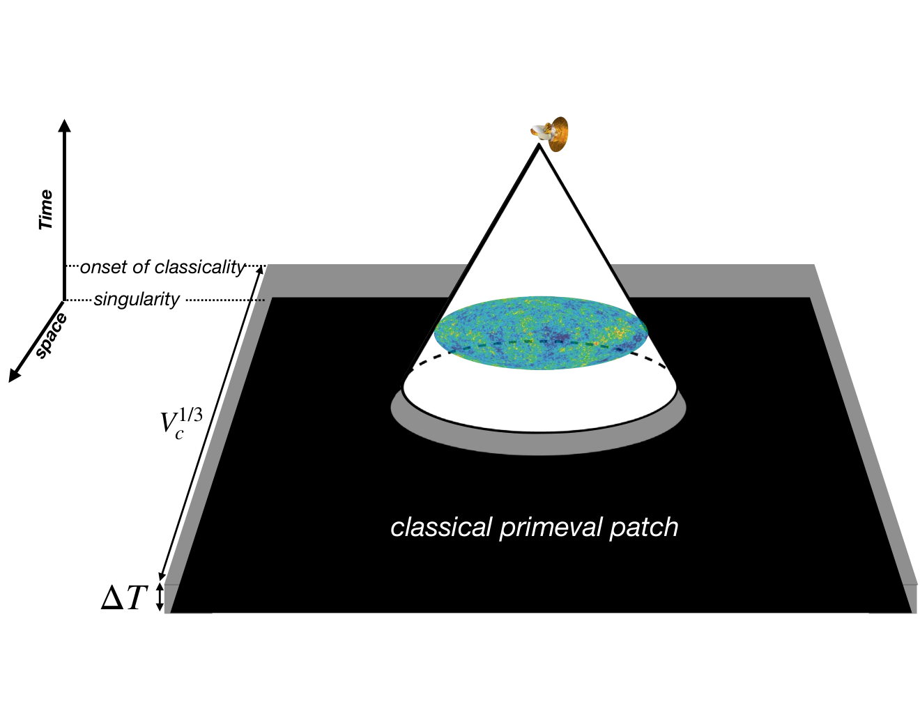
There is an intrinsic infrared cutoff for the size of the classical primeval patch . We can parameterize
(18) with varying from model to model.
We combine all of this into
| (19) |
where and pull in opposite directions and . We can also obtain (17) by setting .
We can now relate unimodular time and redshift via a change of variables:
| (20) |
and use the Friedmann equation to find:
| (21) |
We can also use, under the assumption of adiabatic expansion:
| (22) | |||
| (23) | |||
| (24) |
to obtain:
| (25) |
| (26) |
where we have used the fact that does not change with time. Inserting (19) we arrive at:
| (27) |
so that the Universe can only be classical at the relevant large scales for
| (28) |
For a whole closed Universe this becomes:
| (29) |
For (for ultra-relativistic Standard Model) and , these imply:
| (30) | |||||
or in a closed universe:
| (31) | |||||
which is shown in Figure (2), and compared to the current observational bounds on . As we see, rather than being the Planck scale, the most natural scale for the emergence of classicality in this theory is GeV.
This is the main conclusion in this paper, and the rest of the paper is devoted to refining the argument and checking how robust it might or might not be. This conclusion will be reinforced and vindicated, until at the very end of this paper, where a surprising discovery provides an interesting exception to the rule.
IV Gaussian States in Mini-Superspace
It is possible to confirm the argument in the last Section with explicit dynamical solutions. For a Universe with , matter and radiation, the in (4) must satisfy the Hamiltonian constraint for:
| (32) |
General solutions in the connection representation have been found in Magueijo; Gielen and Magueijo; Alexandre and Magueijo. They can be written as:
| (33) |
for functions which take the simple asymptotic forms:
| (34) | |||||
| (35) | |||||
| (36) |
in the , matter and radiation epochs, respectively (we have ignored the curvature , and highlighted the dependence in via ). Here and are constants which are irrelevant for our purposes. Assuming a sharp Gaussian for we can Taylor expand and explicitly evaluate (4) as:
| (37) |
where
| (38) |
is the monochromatic partial wave for the central value (which is a pure phase), where:
| (39) |
and where:
| (40) |
indeed saturates the Heisenberg bound, and therefore is constant, as assumed in the argument of the previous Section. For the 3 epochs of the Universe we have respectively:
| (41) | |||||
| (42) | |||||
| (43) |
and it can be checked that represents the classical trajectory. This is followed by the peak of the Gaussian, so absence of quantum behavior can be assessed from the induced
| (44) |
following from error propagation and . Thus:
| (45) | |||||
| (46) | |||||
| (47) |
for the 3 epochs in the life of the Universe. Considering that we are just entering the Lambda epoch (so that up to factors of order 1, ), this implies up to factors of order 1:
| (48) |
where we have used (21) in the last step.
Hence not only do the explicit minisuperspace solutions vindicate the essential assumption that is a constant and that its effects translate into uncertainties in the cosmic evolution (in terms of ), but they do not lead to significant numerical corrections.
V Robustness with regards to the choice of function
The choice of (see end of Section II) leads to different quantum theories; indeed the most natural one to emerge from the dynamics is , the “wavenumber” appearing in the Chern-Simons state (cf. Eq.34, see also Kodama 1990; Magueijo 2021b; Magueijo). However, unless is very contrived, this does not affect the discussion in this paper, modulo factors of order 1. For example, for any power-law , if , then, from small error propagation:
| (49) |
and nothing changes qualitatively in our arguments unless or (i.e. making the results applicable to the topical case ). More generally, if a Gaussian is sufficiently sharply peaked, then the distribution of any function of its random variable is also approximately a sharply peaked Gaussian with variance obtained by small error propagation .
So all we need is for to be order 1 at . The arguments in Sections III and IV then follow. A coherent state in is quasi-coherent in any and vice versa. The arguments in Section III follow through because:
| (50) |
Likewise for the arguments in Section IV since:
so that the extra factor in cancels throughout (in the peak trajectory and in ). Obviously we can design functions for which the argument fails because the small error propagation formula breaks down. Any power-law with very large or small would do this. However one might argue that these are very contrived situations.
We can also consider , that is, two cosmological constants entering the Hamiltonian constrain, but only one contributing to the unimodular clock. This could be case of radiative corrections according to some authors Weinberg 1989; Padilla. In this case our argument still does go through. Although does not need to be small ( and have opposite signs), its variance must still be small because:
| (51) |
In other words, the variance in would have to be small with regards to the total Lambda, for the cancellation to leave with . Hence we obtain the same relation between the time of classicality and the total cosmological constant, .
The same is true in the sequester model Kaloper and Padilla 2014; Kaloper et al. 2016, where one removes the space-time average of the trace of the Einstein equations, so that the unimodular is not observable. Although this is true classically, one can only do this within in the semiclassical theory, so that propagates into the observable defined in Kaloper and Padilla 2014; Kaloper et al. 2016 (that is )22 2 Note that if , it would only tighten the constraints obtained here. We defer a full discussion to future work.. Again, the same relation is obtained between and . The situation, however, is complicated by the fact that in Kaloper et al. 2016 there are two clocks (a Ricci clock as well as a unimodular clock), so that a new layer comes into the argument. We defer a full analysis to a future publication.
VI In search of a superhorizon infrared scale
The only leeway we have in our results therefore relates to , the comoving volume of the classical primeval patch, and obviously we would destroy our bound by letting , since then and all uncertainties would go to zero. There is, however, no reason for choosing this, quite the contrary. Indeed in this case the energy scale for classicality would be infinite, that is, at least in the minisuperspace limit the Universe would not be subjected to quantum gravity, even deep in the Planck epoch.
Nonetheless, we use this limit as inspiration for trying to find a physically motivated context in which our bound would emerge weakened, and instead seek a context within which the Planck scale could be the scale of classicality for these theories: . Given that (at least for now) we cannot see beyond the last scattering surface at 13 Gpc, the scale that sets the size of the classical primeval patch only has a firm lower limit. But how big can it really be?
Current observations indicate a red spectrum of primordial scalar perturbations, implying that fluctuations become more nonlinear on large superhorizon scales. Similar to Quantum Chromodynamics (QCD), this may lead to a strong coupling scale in the deep infrared. Following this hypothesis, we will use the solution to the 1-loop renormalization group (RG) equation for a generic renormalizable theory (such as 4D Yang-Mills) to capture running of the scalar power spectrum:
| (52) |
where is the scalar spectral index, and is the conventional pivot scale. We can see that this power spectrum diverges at:
| (53) |
Notice that does not appear in this expression because it concerns a scale for a divergence, therefore erasing any fine tuning that might come from . If we identify this scale with the (inverse of the) size of the classical primeval patch, i.e., (with defined in Equation 18), combining Equations (28) and (53) yields:
| (54) |

Now, imagine we require classicality to emerge somewhere within . This implies:
| (55) |
which is consistent with the current combined Planck 2018 bound: Aghanim et al. 2020.
This is a very surprising result, given that the two numbers, and , are a priori not related at all. The only way to get the Planck scale as the scale of classicality in this model is for the classical patch to be not infinite, but about times the linear size of the current horizon, i.e. precisely the scale that becomes nonlinear given the observed scalar spectral tilt of . This coincidence is depicted in Figure (3).
The qualitative connection between the RG flow of 3D quantum field theories and the cosmological power spectra can be made concrete in the context of McFadden & Skenderis’ Holographic Cosmology program McFadden and Skenderis 2010. In particular, our surprising discovery of the connection between and through the Planck scale points to renormalizable 3D quantum theories (which have logarithimc running), and suggests that the cosmological correlations may be fully described by a finite number of couplings within these theories, which (broadly speaking) includes Chern-Simons 3-form coupling, as well as and Yukawa couplings 33 3 K. Skenderis, private communication.. To the best of our knowledge, determining the classes of these theories that lead to IR confinement (as suggested by our observed value of ), remains an open question.
VII Conclusions
In summary, we have related the value of the cosmological constant and the energy scale for the emergence of classicality in a unimodular universe: A lower bound in the former translating into an upper bound in the latter and vice versa. The argument is robust with respect to many technicalities, with the exception of the choice of the comoving volume taken for the “classical primeval patch” of the Universe. If this is taken to be the current Hubble volume or even the whole of a closed Universe with a small but non-negligible then this scale is naturally around GeV, and not the Planck scale. It would be interesting to relate this number to the amplitude of the fluctuations in inflationary models operating at this energy scale.
A second surprise found in this paper is obtained if we allow ourselves latitude for a much larger patch of classicality, ; specifically setting it to be the scale where the primordial fluctuations become divergent for a red spectrum. While this is not entirely model-independent, it suggests that a very large classical primeval patch can lift the energy scale of classicality to the Planck scale for values of close to the observed ones. Note that if the scale were to be infinite (i.e. if an infinite Universe were to be globally classical), then the energy scale for classicality would be infinite, and not the Planck energy either. Hence it is a remarkable coincidence that the observed values of spectral tilt of and cosmological constant Aghanim et al. 2020 point to a value of that set the energy scale of classicality at the Planck energy. In the context of holographic cosmology McFadden and Skenderis 2010, this coincidence suggests that the holographic 3D quantum field theory that describes our cosmological observations must be a renormalizbale theory with an IR confinement scale of times the current comoving Hubble radius.
So, what next?
On the theoretical front a clearer understanding of what may happen as we approach the scale of the classical primeval patch is required. In the context of our first scenario with GeV, one may be tempted to entertain the rich zoology of eternally inflating models, but intriguingly, a positive curvature with any appreciable (is believed to) rule them out entirely Kleban and Schillo 2012. Qualitatively, it will be hard to reconcile a near-scale invariant spectrum (as observed) with a small scale of non-linearity comparable to Hubble radius in any model. Nonetheless, interesting lessons may be learnt from 3D lattice simulations Cossu et al. 2021 in the context of super-renormalizble holographic dual theories (e.g., McFadden and Skenderis 2010; Afshordi et al. 2017a; Afshordi et al. 2017b). A less-charted, but potentially more fertile territory may be a systematic study of the RG flows in renormalizable 3D quantum field theories that manifest confinement in the IR, and connects to our second scenario with . At a more foundational level, one may wonder whether there exists a holographic interpretation of the unimodular gravity.
On the observational front, there will be “dragons” (or other new physics) beyond the cosmological horizon. Indeed, in the first scenario, the quantum cosmology dragons should be in our face and right around the corner. Maybe an explanation for the infamous CMB anomalies Akrami et al. 2020 such as “The axis of evil” Land and Magueijo 2005, “Planck Evidence for a closed Universe” Handley 2021; Di Valentino et al. 2019 (Figure 2), or rather more subtle “cosmological zero modes” Afshordi and Johnson 2018 could be their tail? The fingerprints of the second scenario will be more subtle, but also more robust. For example, Equation (52) predicts the running of the spectral index to be , setting a clear target for the next generation of cosmological surveys (e.g., Li et al. 2018). Furthermore, we expect the same IR strong coupling scale, (Eq. 53) for both scalar and tensor modes. Therefore, using the same functional form as Equation (52) for tensors, we further can predict the tilt for tensors (should they ever be detected).
The two scenarios are certainly distinguishable and falsifiable separately. For example, the observation of topological defects left over from a phase transition at an energy scale above GeV would kill the first scenario (but we are not holding our breath). Furthermore, given that such low scale of classicality only allows for low-scale inflation, then inflationary modes should be unobservable44 4 We thank Tony Padilla for pointing this out.. There are also other intriguing but very model-dependent possibilities for the first scenario, for example regarding the amplitude of scalar fluctuations. The ratio between and the Planck scale is then , not too different from . Could the value of and that the amplitude of the primordial fluctuations be related?
We close with general comments regarding other work on the cosmological constant. We note that the argument we presented here gives a (minimal) width for the distribution of , and not its central value, solving what Weinberg referred to as the “new cosmological constant problem” Weinberg. The “old cosmological problem” of why is contained within (or at the centre) of this distribution may find a solution through the non-perturbative structure of quantum gravity (e.g., Hawking 1984; Afshordi; Aslanbeigi et al. 2011; Kaloper and Westphal). We note also that the scale could appear in the variance itself, as happens in causal set models Sorkin 2003; Ahmed et al. 2004; Zwane et al. 2018, where is a Poissonian process. This does not affect our argument, since the point made here is that must be smaller than the central value on whatever scale of classicality, , we have defined.
Acknowledgements.
We thank Bruno Alexandre, Davide Gaiotto, Tony Padilla, and Kostas Skenderis for discussions related to this paper. NA is funded by the University of Waterloo, the National Science and Engineering Research Council of Canada (NSERC) and the Perimeter Institute for Theoretical Physics. Research at Perimeter Institute is supported by the Government of Canada through Industry Canada and by the Province of Ontario through the Ministry of Economic Development & Innovation. JM is funded by the STFC Consolidated Grant ST/T000791/1. JM also thanks the Perimeter Institute for hospitality and support.References
- Unruh (1989) W. G. Unruh, Phys. Rev. D 40, 1048 (1989).
- Smolin (2009) L. Smolin, Phys. Rev. D 80 (2009), arXiv:0904.4841 .
- Kuchař (1991) K. V. Kuchař, Phys. Rev. D 43, 3332 (1991).
- Henneaux and Teitelboim (1989) M. Henneaux and C. Teitelboim, Phys. Lett. B 222, 195 (1989).
- Carballo-Rubio et al. (2022) R. Carballo-Rubio, L. J. Garay, and G. García-Moreno, (2022), arXiv:2207.08499 [gr-qc] .
- Weinberg (1989) S. Weinberg, Rev. Mod. Phys. 61, 1 (1989).
- (7) A. Padilla, 1502, arXiv:1502.05296 .
- Kaloper and Padilla (2014) N. Kaloper and A. Padilla, Phys. Rev. Lett 112 (2014), arXiv:1309.6562 .
- Kaloper et al. (2016) N. Kaloper, A. Padilla, D. Stefanyszyn, and G. Zahariade, Phys. Rev. Lett 116 (2016), arXiv:1505.01492 .
- Bombelli et al. (1991) L. Bombelli, W. E. Couch, and R. J. Torrence, Phys. Rev. D 44, 2589 (1991).
- Smolin (2011) L. Smolin, Phys. Rev. D 84, 044047 (2011), arXiv:1008.1759 [hep-th] .
- Misner (1969) C. W. Misner, Phys Rev. 186 (1969).
- Gielen and Menéndez-Pidal (2022) S. Gielen and L. Menéndez-Pidal, Class. Quant. Grav. 39, 075011 (2022), arXiv:2109.02660 [gr-qc] .
- Magueijo (2021a) J. Magueijo, Phys. Lett. B 820, 136487 (2021a), arXiv:2104.11529 [gr-qc] .
- (15) J. Magueijo, Phys. Rev. D in press, arXiv::2110.05920 .
- (16) S. Gielen and J. Magueijo, Quantum analysis of the recent cosmological bounce in comoving Hubble length, arXiv:2201.03596 [[gr-qc]] .
- (17) B. Alexandre and J. Magueijo, arXiv:2207.03854 [[gr-qc]] .
- Alexandre and Magueijo (2021) B. Alexandre and J. Magueijo, Rev. D 104, 124069 (2021), arXiv:2110.10835 [[gr-qc]] .
- Aghanim et al. (2020) N. Aghanim et al. (Planck), Astron. Astrophys. 641, A6 (2020), [Erratum: Astron.Astrophys. 652, C4 (2021)], arXiv:1807.06209 [astro-ph.CO] .
- Handley (2021) W. Handley, Phys. Rev. D 103, L041301 (2021), arXiv:1908.09139 [astro-ph.CO] .
- Di Valentino et al. (2019) E. Di Valentino, A. Melchiorri, and J. Silk, Nature Astron. 4, 196 (2019), arXiv:1911.02087 [astro-ph.CO] .
- Kodama (1990) H. Kodama, Phys. Rev. D 42, 2548 (1990).
- Magueijo (2021b) J. Magueijo, Phys. Rev. D 104, 026002 (2021b), arXiv:2012.05847 [[gr-qc]] .
- McFadden and Skenderis (2010) P. McFadden and K. Skenderis, Phys. Rev. D 81 (2010), 10.1103/PhysRevD.81.021301, arXiv:0907.5542 [[hep-th]] .
- Kleban and Schillo (2012) M. Kleban and M. Schillo, JCAP 6 (2012), 10.1088/1475-7516/2012/06/029, arXiv:1202.5037 .
- Cossu et al. (2021) G. Cossu, L. D. Debbio, A. Juttner, B. Kitching-Morley, J. K. L. Lee, A. Portelli, H. B. Rocha, and K. Skenderis, Phys. Rev. Lett. 126, 221601 (2021), arXiv:2009.14768 [[hep-lat]] .
- Afshordi et al. (2017a) N. Afshordi, C. Coriano, L. D. Rose, E. Gould, and K. Skenderis, Phys. Rev. Lett. 118, 041301 (2017a), arXiv:1607.04878 [[astro-ph.CO]] .
- Afshordi et al. (2017b) N. Afshordi, E. Gould, and K. Skenderis, Phys. Rev. D 95, 123505 (2017b), arXiv:1703.05385 [ [astro-ph.CO]] .
- Akrami et al. (2020) Y. Akrami et al. (Planck), Astron. Astrophys. 641, A7 (2020), arXiv:1906.02552 [astro-ph.CO] .
- Land and Magueijo (2005) K. Land and J. Magueijo, Phys. Rev. Lett. 95, 071301 (2005), arXiv:astro-ph/0502237 .
- Afshordi and Johnson (2018) N. Afshordi and M. C. Johnson, Phys. Rev. D 98, 023541 (2018), arXiv:1708.04694 [astro-ph.CO] .
- Li et al. (2018) X. Li, N. Weaverdyck, S. Adhikari, D. Huterer, J. Muir, and H.-Y. Wu, Astrophys. J. 862, 137 (2018), arXiv:1806.02515 [astro-ph.CO] .
- (33) S. Weinberg, arXiv:astro-ph/0005265 [ [astro-ph]] .
- Hawking (1984) S. W. Hawking, Phys. Lett. B 134, 403 (1984).
- (35) N. Afshordi, arXiv:0807.2639 [[astro-ph]] .
- Aslanbeigi et al. (2011) S. Aslanbeigi, G. Robbers, B. Z. Foster, K. Kohri, and N. Afshordi, Phys Rev. D 84 (2011), 10.1103/PhysRevD.84.103522, arXiv:1106.3955 [[astro-ph.CO]] .
- (37) N. Kaloper and A. Westphal, arXiv:2204.13124 [[hep-th]] .
- Sorkin (2003) R. D. Sorkin, in School on Quantum Gravity (2003) pp. 305–327, arXiv:gr-qc/0309009 .
- Ahmed et al. (2004) M. Ahmed, S. Dodelson, P. B. Greene, and R. Sorkin, Phys. Rev. D 69, 103523 (2004), arXiv:astro-ph/0209274 .
- Zwane et al. (2018) N. Zwane, N. Afshordi, and R. D. Sorkin, Class. Quant. Grav. 35, 194002 (2018), arXiv:1703.06265 [gr-qc] .