跳到论文正文
W Papers独立论文阅读器 arXiv:2209.07715 论文正文 计算阅读时间 · 0%
引用这篇论文根据当前论文元数据生成,正式投稿前建议核对。


License: CC BY-NC-ND 4.0
arXiv:2209.07715v1 [cs.AI] 16 Sep 2022

Comments on “Iteratively Re-Weighted Algorithm for Fuzzy c-Means”

Astha Saini    Prabhu Babu Thanks: Astha Saini and Prabhu Babu are with the Centre for Applied Research in Electronics, Indian Institute of Technology Delhi, New Delhi 110016, India (e-mail: astha.saini@care.iitd.ac.in, prabhu.babu@care.iitd.ac.in).
Abstract

In this comment, we present a simple alternate derivation to the IRW-FCM algorithm presented in [1] for Fuzzy c-Means problem. We show that the iterative steps derived in [1] are nothing but steps of the popular Majorization Minimization (MM) algorithm. The derivation presented in this note is much simpler and straightforward and, unlike the derivation in [1], the derivation here does not involve introduction of any auxiliary variable. Moreover, by showing the steps of IRW-FCM as the MM algorithm, the inner loop of the IRW-FCM algorithm can be eliminated and the algorithm can be effectively run as a “single loop” algorithm. More precisely, the new MM-based derivation deduces that a single inner loop of IRW-FCM is sufficient to decrease the Fuzzy c-means objective function, which speeds up the IRW-FCM algorithm.

Index Terms:
Fuzzy c-Means, IRW-FCM, MM Algorithm.

I Introduction and IRW-FCM Algorithm

Following the notations used in [1], let 𝐱1,𝐱2,…..,𝐱n{\mathbf{x}_{1},\mathbf{x}_{2},.....,\mathbf{x}_{n}} denote the data points that have to be divided into ‘cc’ clusters with centers {𝐦j}j=1c\{\mathbf{m}_{j}\}_{j=1}^{c}, and fi​jf_{ij} denote the (i,j)th(i,j)^{\text{th}} element of the membership matrix 𝐅\mathbf{F} which indicates the membership of the ithi^{\text{th}} data point to the jthj^{\text{th}} cluster. It is obvious that the elements of 𝐅\mathbf{F} have to be non-negative and unlike the K-Means clustering technique, which requires the elements of 𝐅\mathbf{F} to be either 0 or 1, in the case of Fuzzy clustering the elements of 𝐅\mathbf{F} can be between 0 and 1 but the sum of elements in any row of 𝐅\mathbf{F} should be equal to 1, i.e., 𝐅𝟏=𝟏\mathbf{F1}=\mathbf{1}. With this, the Fuzzy c-Means problem can be stated as follows:

min𝐅𝟏=𝟏,𝐅≥0,{𝐦j}∑j=1c∑i=1nfi​jr∥𝐱i−𝐦j∥22,\displaystyle\min_{\mathbf{F1}=\mathbf{1},\mathbf{F}\geq 0,\{\mathbf{m}_{j}\}}\sum_{j=1}^{c}\sum_{i=1}^{n}f_{ij}^{r}\|\mathbf{x}_{i}-\mathbf{m}_{j}\|_{2}^{2},
min𝐅𝟏=𝟏,𝐅≥0,{𝐦j}∑j=1c∑i=1nfi​jr(𝐱iT𝐱i−2𝐱iT𝐦j+𝐦jT𝐦j).\displaystyle\min_{\mathbf{F1}=\mathbf{1},\mathbf{F}\geq 0,\{\mathbf{m}_{j}\}}\sum_{j=1}^{c}\sum_{i=1}^{n}f_{ij}^{r}(\mathbf{x}_{i}^{T}\mathbf{x}_{i}-2\mathbf{x}_{i}^{T}\mathbf{m}_{j}+\mathbf{m}_{j}^{T}\mathbf{m}_{j}). (1)

The parameter rr in (I) indicates the level of fuzziness in the clustering. A usual approach to solve (I) is to use alternating minimization, i.e., for a fixed 𝐅\mathbf{F}, update {𝐦j\mathbf{m}_{j}} and vice-versa. For a fixed 𝐅\mathbf{F}, the minimizer over {𝐦j\mathbf{m}_{j}} is given by:

𝐦j=∑i=1nfi​jr​𝐱i∑i=1nfi​jr=∑i=1ngi​j​𝐱i∑i=1ngi​j=𝐗𝐠j𝐠jT​𝟏,\mathbf{m}_{j}=\frac{\sum_{i=1}^{n}f_{ij}^{r}\mathbf{x}_{i}}{\sum_{i=1}^{n}f_{ij}^{r}}=\frac{\sum_{i=1}^{n}g_{ij}\mathbf{x}_{i}}{\sum_{i=1}^{n}g_{ij}}=\frac{\mathbf{X}\mathbf{g}_{j}}{\mathbf{g}_{j}^{T}\mathbf{1}}, (2)

where gi​j=fi​jrg_{ij}=f_{ij}^{r}. With fixed {𝐦j\mathbf{m}_{j}}, solving for 𝐅\mathbf{F} via the Lagrange Multiplier method with the constraint ∑j=1cfi​j=1\sum_{j=1}^{c}f_{ij}=1 gives:

fi​j=di​j(21−r)∑k=1cdi​k(21−r),f_{ij}=\frac{d_{ij}^{(\frac{2}{1-r})}}{\sum_{k=1}^{c}d_{ik}^{(\frac{2}{1-r})}}, (3)

where di​j=‖𝐱i−𝐦j‖2d_{ij}=\|\mathbf{x}_{i}-\mathbf{m}_{j}\|_{2}. The alternating steps of (2) and (3) is known as FCM algorithm [2]. In [1], the authors have stated that the FCM algorithm suffers from convergence to sub-optimal minimum by blaming the alternating approach of FCM, and they proposed a new algorithm named IRW-FCM, that minimizes an equivalent problem of (I). More precisely, they obtained a problem only in 𝐅\mathbf{F} by substituting for the optimal minimizer over {𝐦j\mathbf{m}_{j}} (from (2)) in (I) and obtained the equivalent problem as shown below:

min𝐅𝟏=𝟏,𝐅≥0\displaystyle\min_{\mathbf{F1}=\mathbf{1},\mathbf{F}\geq 0} ϕ⁡({𝐠j})=△\displaystyle\phi(\{\mathbf{g}_{j}\})\stackrel{{\scriptstyle{\tiny\triangle}}}{{=}}
∑j=1c∑i=1ngi​j​𝐱iT​𝐱i−∑j=1c(𝐠jT​𝐗T​𝐗𝐠j𝐠jT​𝟏),\displaystyle\sum_{j=1}^{c}\sum_{i=1}^{n}g_{ij}\mathbf{x}_{i}^{T}\mathbf{x}_{i}-\sum_{j=1}^{c}\left(\frac{\mathbf{g}_{j}^{T}\mathbf{X}^{T}\mathbf{X}\mathbf{g}_{j}}{\mathbf{g}_{j}^{T}\mathbf{1}}\right), (4)

which they solved as follows. First, they introduced an auxiliary variable 𝐬∈ℝc×1\mathbf{s}\in\mathbb{R}^{c\times 1} and came up with a problem in {𝐠j}\{\mathbf{g}_{j}\} and 𝐬\mathbf{s}, which is equivalent to (I):

min𝐅𝟏=𝟏,𝐅≥0,𝐬⁡ψ⁡({𝐠j},𝐬)=△∑j=1c∑i=1ngi​j​𝐱iT​𝐱i+∑j=1c(sj2​𝐠jT​𝟏−2​sj​𝐠jT​𝐗T​𝐗𝐠j).\begin{split}&\min_{\mathbf{F1}=\mathbf{1},\mathbf{F}\geq 0,\mathbf{s}}\psi(\{\mathbf{g}_{j}\},\mathbf{s})\stackrel{{\scriptstyle{\tiny\triangle}}}{{=}}\\ &\sum_{j=1}^{c}\sum_{i=1}^{n}g_{ij}\mathbf{x}_{i}^{T}\mathbf{x}_{i}+\sum_{j=1}^{c}(s_{j}^{2}\mathbf{g}_{j}^{T}\mathbf{1}-2s_{j}\sqrt{\mathbf{g}_{j}^{T}\mathbf{X}^{T}\mathbf{X}\mathbf{g}_{j}}).\end{split} (5)

For a fixed 𝐅\mathbf{F}, the optimal minimizer over 𝐬\mathbf{s} is given by {sj=𝐠jT​𝐗T​𝐗𝐠j𝐠jT​𝟏}\left\{s_{j}=\frac{\sqrt{\mathbf{g}_{j}^{T}\mathbf{X}^{T}\mathbf{X}\mathbf{g}_{j}}}{\mathbf{g}_{j}^{T}\mathbf{1}}\right\}, and substituting it back in (5), we get (I) and this proves the equivalence of (I) and (5). Then they proposed to solve (5) via alternating minimization: For fixed 𝐬\mathbf{s}, update 𝐅\mathbf{F} and vice-versa. For a fixed 𝐬\mathbf{s} (say 𝐬t+1\mathbf{s}^{t+1} computed using 𝐅t\mathbf{F}^{t}), the minimization problem over 𝐅\mathbf{F} is given by:

min𝐅𝟏=𝟏,𝐅≥0∑j=1c∑i=1ngi​j​𝐱iT​𝐱i+∑j=1c((sjt+1)2​𝐠jT​𝟏−2​sjt+1​𝐠jT​𝐗T​𝐗𝐠j).\begin{split}\min_{\mathbf{F1}=\mathbf{1},\mathbf{F}\geq 0}&\sum_{j=1}^{c}\sum_{i=1}^{n}g_{ij}\mathbf{x}_{i}^{T}\mathbf{x}_{i}+\\ &\sum_{j=1}^{c}\left((s_{j}^{t+1})^{2}\mathbf{g}_{j}^{T}\mathbf{1}-2s_{j}^{t+1}\sqrt{\mathbf{g}_{j}^{T}\mathbf{X}^{T}\mathbf{X}\mathbf{g}_{j}}\right).\end{split} (6)

However, (6) does not have any closed form solution, so they resorted to another optimization strategy named IRW[3], which approximates the negative square root function −𝐠jT​𝐗T​𝐗𝐠j-\sqrt{\mathbf{g}_{j}^{T}\mathbf{X}^{T}\mathbf{X}\mathbf{g}_{j}} in (6) with a linear function at some given 𝐅t\mathbf{F}^{t}, and solved the following approximated problem:

min𝐅𝟏=𝟏,𝐅≥0∑j=1c∑i=1ngi​j𝐱iT𝐱i+∑j=1c((sjt+1)2𝟏T𝐠j−2sjt+1𝐚jT𝐠j),\min_{\mathbf{F1}=\mathbf{1},\mathbf{F}\geq 0}\sum_{j=1}^{c}\sum_{i=1}^{n}g_{ij}\mathbf{x}_{i}^{T}\mathbf{x}_{i}+\sum_{j=1}^{c}((s_{j}^{t+1})^{2}\mathbf{1}^{T}\mathbf{g}_{j}-2s_{j}^{t+1}\mathbf{a}_{j}^{T}\mathbf{g}_{j}), (7)

where 𝐚j=𝐗T​𝐗𝐠jt(𝐠jt)T​𝐗T​𝐗𝐠jt\mathbf{a}_{j}=\frac{\mathbf{X}^{T}\mathbf{X}\mathbf{g}_{j}^{t}}{\sqrt{(\mathbf{g}_{j}^{t})^{T}\mathbf{X}^{T}\mathbf{X}\mathbf{g}_{j}^{t}}}. The problem in (7) has a closed form solution given by:

fi​jt+1=(𝐱iT​𝐱i+(sjt+1)2−2​sjt+1​ai​j)11−r∑k=1c(𝐱iT​𝐱i+(skt+1)2−2​skt+1​ai​k)11−r.f_{ij}^{t+1}=\frac{(\mathbf{x}_{i}^{T}\mathbf{x}_{i}+(s_{j}^{t+1})^{2}-2s_{j}^{t+1}a_{ij})^{\frac{1}{1-r}}}{\sum_{k=1}^{c}(\mathbf{x}_{i}^{T}\mathbf{x}_{i}+(s_{k}^{t+1})^{2}-2s_{k}^{t+1}a_{ik})^{\frac{1}{1-r}}}. (8)

Thus, the IRW-FCM approach which solves (I) is iterative, and effectively it is a “double loop” algorithm (one loop for alternating minimization and second inner loop for IRW procedure) as summarized in Algorithm 1.

Algorithm 1 IRW-FCM Algorithm
 Input(𝐗,c)(\mathbf{X},c)
 Initialize 𝐅0\mathbf{F}^{0}
 repeat
     Calculate {sjt+1}\{s_{j}^{t+1}\}
     repeat
      Calculate 𝐚j\mathbf{a}_{j}
      Calculate 𝐅\mathbf{F} using equation (8)
     until convergence, Output 𝐅t+1\mathbf{F}^{t+1}
 until convergence
 Output 𝐅∗\mathbf{F}^{*}, 𝐅∗\mathbf{F}^{*} denotes the optimal minimizer.

II MM BASED DERIVATION

The authors of [1] criticised the alternating minimization approach of FCM by saying that it suffers from convergence to sub-optimal minimum and motivated to solve the equivalent problem in (I) to avoid any such issues. However, in the process of solving (I) they “reversed back” and introduced a new auxiliary variable and again relied on the alternating minimization approach to solve the equivalent problem in (5). Moreover, they had to resort to a separate iterative procedure of IRW to solve one of the subproblems of the alternating minimization, which results in a “double-loop” algorithm.

In the following, we are going to present a much straightforward procedure in which we try and derive an iterative algorithm to solve (I) by working only with the variable of interest (𝐅\mathbf{F}). We will employ a popular approach named Majorization-Minimization (MM)[4] to accomplish this. Before we venture into solving the problem in (I), we first briefly introduce the MM approach. Let us say that we are interested in minimizing a function f⁡(𝐱)f(\mathbf{x}) over a domain χ\mathbf{\chi}, MM does the job in two steps: In the first step, given some 𝐱t\mathbf{x}^{t} (𝐱t∈χ\mathbf{x}^{t}\in\mathbf{\chi}), it constructs a tighter upperbound h⁡(𝐱|𝐱t)h(\mathbf{x}|\mathbf{x}^{t}) to the cost function f⁡(𝐱)f(\mathbf{x}), and in the second step it minimizes the upperbound h⁡(𝐱|𝐱t)h(\mathbf{x}|\mathbf{x}^{t}) w.r.t. 𝐱\mathbf{x} and obtains the next iterate 𝐱t+1\mathbf{x}^{t+1} and this is repeated till convergence. The upperbound h⁡(𝐱|𝐱t)h(\mathbf{x}|\mathbf{x}^{t}) should satisfy the following properties:

f⁡(𝐱t)=h⁡(𝐱t|𝐱t),and​f​(𝐱)≤h⁡(𝐱|𝐱t)​∀𝐱∈χ.f(\mathbf{x}^{t})=h(\mathbf{x}^{t}|\mathbf{x}^{t}),\text{and}\>f(\mathbf{x})\leq h(\mathbf{x}|\mathbf{x}^{t})\;\;\forall\,\mathbf{x}\in\mathbf{\chi}. (9)

It is easy to verify that the series of iterates obtained via MM will monotonically decrease the objective as shown below:

f⁡(𝐱t+1)≤h⁡(𝐱t+1|𝐱t)≤h⁡(𝐱t|𝐱t)=f⁡(𝐱t).f(\mathbf{x}^{t+1})\leq h(\mathbf{x}^{t+1}|\mathbf{x}^{t})\leq h(\mathbf{x}^{t}|\mathbf{x}^{t})=f(\mathbf{x}^{t}). (10)

The first inequality in (10) is due to (9) and the second inequality is due to fact that 𝐱t+1\mathbf{x}^{t+1} is obtained by minimizing h⁡(𝐱|𝐱t)h(\mathbf{x}|\mathbf{x}^{t}), and the last equality is also due to (9). Now, coming back to problem in (I), it is easy to see that the second term (without the negative sign) in (I) is a quadratic over linear function (with 𝐠jT​𝟏>0\mathbf{g}_{j}^{T}\mathbf{1}>0), which is a convex function (see section 3.1.5 in [5]) or, in other words, the function −𝐠jT​𝐗T​𝐗𝐠j𝐠jT​𝟏-\frac{\mathbf{g}_{j}^{T}\mathbf{X}^{T}\mathbf{X}\mathbf{g}_{j}}{\mathbf{g}_{j}^{T}\mathbf{1}} is a concave function in ‘𝐠j\mathbf{g}_{j}’. Thus a tighter upperbound (at a given 𝐅t\mathbf{F}^{t}) can be obtained via a tangent hyperplane passing through 𝐅t\mathbf{F}^{t}, which of course can be obtained via first order Taylor series expansion as shown below:

−𝐠jT​𝐗T​𝐗𝐠j𝐠jT​𝟏≤−(𝐠jt)T​𝐗T​𝐗𝐠jt(𝐠jt)T​𝟏−[2​(𝐠jt)T​𝟏​(𝐠jt)T​𝐗T​𝐗−(𝐠jt)T​𝐗T​𝐗𝐠jt​𝟏T𝟏T​𝐠jt​(𝐠jt)T​𝟏​(𝐠j−𝐠jt)],\begin{split}&-\frac{\mathbf{g}_{j}^{T}\mathbf{X}^{T}\mathbf{X}\mathbf{g}_{j}}{\mathbf{g}_{j}^{T}\mathbf{1}}\leq-\frac{(\mathbf{g}_{j}^{t})^{T}\mathbf{X}^{T}\mathbf{X}\mathbf{g}_{j}^{t}}{(\mathbf{g}_{j}^{t})^{T}\mathbf{1}}\;-\\ &\bigg[\frac{2(\mathbf{g}_{j}^{t})^{T}\mathbf{1}(\mathbf{g}_{j}^{t})^{T}\mathbf{X}^{T}\mathbf{X}-(\mathbf{g}_{j}^{t})^{T}\mathbf{X}^{T}\mathbf{X}\mathbf{g}_{j}^{t}\mathbf{1}^{T}}{\mathbf{1}^{T}\mathbf{g}_{j}^{t}(\mathbf{g}_{j}^{t})^{T}\mathbf{1}}(\mathbf{g}_{j}-\mathbf{g}_{j}^{t})\bigg],\end{split} (11)

with equality achieved at 𝐠j=𝐠jt\mathbf{g}_{j}=\mathbf{g}_{j}^{t}.The MM upperbound for the objective in (I) at some given (𝐅t)(\mathbf{F}^{t}) is then given by:

ϕ({𝐠j})≤∑j=1c∑i=1ngi​j𝐱iT𝐱i−∑j=1c[(𝐠jt)T​𝐗T​𝐗𝐠jt(𝐠jt)T​𝟏+\displaystyle\phi(\{\mathbf{g}_{j}\})\leq\sum_{j=1}^{c}\sum_{i=1}^{n}g_{ij}\mathbf{x}_{i}^{T}\mathbf{x}_{i}-\sum_{j=1}^{c}\bigg[\frac{(\mathbf{g}_{j}^{t})^{T}\mathbf{X}^{T}\mathbf{X}\mathbf{g}_{j}^{t}}{(\mathbf{g}_{j}^{t})^{T}\mathbf{1}}\;+
2​(𝐠jt)T​𝟏​(𝐠jt)T​𝐗T​𝐗−(𝐠jt)T​𝐗T​𝐗𝐠jt​𝟏T𝟏T​𝐠jt​(𝐠jt)T​𝟏(𝐠j−𝐠jt)]\displaystyle\frac{2(\mathbf{g}_{j}^{t})^{T}\mathbf{1}(\mathbf{g}_{j}^{t})^{T}\mathbf{X}^{T}\mathbf{X}-(\mathbf{g}_{j}^{t})^{T}\mathbf{X}^{T}\mathbf{X}\mathbf{g}_{j}^{t}\mathbf{1}^{T}}{\mathbf{1}^{T}\mathbf{g}_{j}^{t}(\mathbf{g}_{j}^{t})^{T}\mathbf{1}}(\mathbf{g}_{j}-\mathbf{g}_{j}^{t})\bigg]
=△h⁡({𝐠j}|{𝐠jt}).\displaystyle\stackrel{{\scriptstyle{\tiny\triangle}}}{{=}}h(\{\mathbf{g}_{j}\}|\{\mathbf{g}_{j}^{t}\}). (12)

Then, the upperbound minimization problem to be solved is given by:

min𝐅𝟏=𝟏,𝐅≥0⁡h⁡({𝐠j}|{𝐠jt})=∑j=1c∑i=1ngi​j​𝐱iT​𝐱i−∑j=1c[2​(𝐠jt)T​𝐗T​𝐗𝐠j(𝐠jt)T​𝟏−(𝐠jt)T​𝐗T​𝐗𝐠jt​𝟏T​𝐠j𝟏T​𝐠jt​(𝐠jt)T​𝟏]+const.\begin{split}&\min_{\mathbf{F1}=\mathbf{1},\mathbf{F}\geq 0}h(\{\mathbf{g}_{j}\}|\{\mathbf{g}_{j}^{t}\})=\sum_{j=1}^{c}\sum_{i=1}^{n}g_{ij}\mathbf{x}_{i}^{T}\mathbf{x}_{i}-\\ &\sum_{j=1}^{c}\bigg[2\frac{(\mathbf{g}_{j}^{t})^{T}\mathbf{X}^{T}\mathbf{X}\mathbf{g}_{j}}{(\mathbf{g}_{j}^{t})^{T}\mathbf{1}}-\frac{(\mathbf{g}_{j}^{t})^{T}\mathbf{X}^{T}\mathbf{X}\mathbf{g}_{j}^{t}\mathbf{1}^{T}\mathbf{g}_{j}}{\mathbf{1}^{T}\mathbf{g}_{j}^{t}(\mathbf{g}_{j}^{t})^{T}\mathbf{1}}\bigg]+\text{const.}\end{split} (13)

Leaving out the constant terms, we get

min𝐅𝟏=𝟏,𝐅≥0∑j=1c∑i=1ngi​j​𝐱iT​𝐱i−∑j=1c[2​(𝐠jt)T​𝐗T​𝐗𝐠j(𝐠jt)T​𝟏−(𝐠jt)T​𝐗T​𝐗𝐠jt​𝟏T​𝐠j𝟏T​𝐠jt​(𝐠jt)T​𝟏],\begin{split}\min_{\mathbf{F1}=\mathbf{1},\mathbf{F}\geq 0}&\sum_{j=1}^{c}\sum_{i=1}^{n}g_{ij}\mathbf{x}_{i}^{T}\mathbf{x}_{i}\;-\\ &\sum_{j=1}^{c}\bigg[2\frac{(\mathbf{g}_{j}^{t})^{T}\mathbf{X}^{T}\mathbf{X}\mathbf{g}_{j}}{(\mathbf{g}_{j}^{t})^{T}\mathbf{1}}-\frac{(\mathbf{g}_{j}^{t})^{T}\mathbf{X}^{T}\mathbf{X}\mathbf{g}_{j}^{t}\mathbf{1}^{T}\mathbf{g}_{j}}{\mathbf{1}^{T}\mathbf{g}_{j}^{t}(\mathbf{g}_{j}^{t})^{T}\mathbf{1}}\bigg],\end{split} (14)

which has a simple closed form solution given by:

fi​jt+1=[𝐱iT​𝐱i+(𝐠jt)T​𝐗T​𝐗𝐠jt𝟏T​𝐠jt​(𝐠jt)T​𝟏−2​𝐱iT​𝐗𝐠jt(𝐠jt)T​𝟏]11−r∑k=1c[𝐱iT​𝐱i+(𝐠kt)T​𝐗T​𝐗𝐠kt𝟏T​𝐠kt​(𝐠kt)T​𝟏−2​𝐱iT​𝐗𝐠kt(𝐠kt)T​𝟏]11−r​∀i,j.f_{ij}^{t+1}=\frac{\left[\mathbf{x}_{i}^{T}\mathbf{x}_{i}+\frac{(\mathbf{g}_{j}^{t})^{T}\mathbf{X}^{T}\mathbf{X}\mathbf{g}_{j}^{t}}{\mathbf{1}^{T}\mathbf{g}_{j}^{t}(\mathbf{g}_{j}^{t})^{T}\mathbf{1}}-2\frac{\mathbf{x}_{i}^{T}\mathbf{X}\mathbf{g}_{j}^{t}}{(\mathbf{g}_{j}^{t})^{T}\mathbf{1}}\right]^{\frac{1}{1-r}}}{\sum_{k=1}^{c}\left[\mathbf{x}_{i}^{T}\mathbf{x}_{i}+\frac{(\mathbf{g}_{k}^{t})^{T}\mathbf{X}^{T}\mathbf{X}\mathbf{g}_{k}^{t}}{\mathbf{1}^{T}\mathbf{g}_{k}^{t}(\mathbf{g}_{k}^{t})^{T}\mathbf{1}}-2\frac{\mathbf{x}_{i}^{T}\mathbf{X}\mathbf{g}_{k}^{t}}{(\mathbf{g}_{k}^{t})^{T}\mathbf{1}}\right]^{\frac{1}{1-r}}}\forall{i,j}. (15)

If one takes a closer look at the problem in (14), it is nothing but the problem in (7) with choice of sjt+1=(𝐠jt)T​𝐗T​𝐗𝐠jt(𝐠jt)T​𝟏s_{j}^{t+1}=\frac{\sqrt{(\mathbf{g}_{j}^{t})^{T}\mathbf{X}^{T}\mathbf{X}\mathbf{g}_{j}^{t}}}{(\mathbf{g}_{j}^{t})^{T}\mathbf{1}}, 𝐚j=𝐗T​𝐗𝐠jt(𝐠jt)T​𝐗T​𝐗𝐠jt\mathbf{a}_{j}=\frac{\mathbf{X}^{T}\mathbf{X}\mathbf{g}_{j}^{t}}{\sqrt{(\mathbf{g}_{j}^{t})^{T}\mathbf{X}^{T}\mathbf{X}\mathbf{g}_{j}^{t}}}. This in a way proves that the iterative steps of IRW-FCM can be easily derived via the MM approach, and more importantly, the inner loop of IRW-FCM algorithm can be run only for one time and that is sufficient to decrease the cost function in (I).

Sr. No. FCM-MM FCM-IRW
1. Single loop algorithm. Double loop algorithm.
2. Does not involve introduction of any auxiliary variable therefore has less space complexity. Requires auxiliary variables and therefore requires more storage.
3. Faster than FCM-IRW as it is equivalent to FCM-IRW with the inner loop run only one time. Slower due to the redundant inner loop.
Table I: DIFFERENCES AND SIMILARITIES BETWEEN FCM-MM AND FCM-IRW ALGORITHMS

III Numerical Simulation Results

Refer to caption
(a)
Refer to caption
(b)
Refer to caption
(c)
Refer to caption
(d)
Refer to caption
(e)
Refer to caption
(f)
Refer to caption
(g)
Refer to caption
(h)
Refer to caption
(i)
Refer to caption
(j)
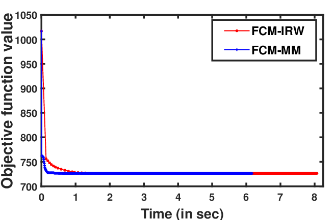
Figure 1: Convergence curves for IRW-FCM and FCM-MM with same initialization on 5 datasets (1(a)) Iris, (1(b)) Audit, (1(c)) Automobile, (1(d)) Haberman Survival, (1(e)) UCIHAR, (1(f)) SCADI, (1(g)) Data Cortex Nuclear, (1(h)) Gesture Phase Segmentation (Processed), (1(i)) EEG Eye State and (1(j)) HTRU2.
Refer to caption
(a)
Refer to caption
(b)
Refer to caption
(c)
Refer to caption
(d)
Refer to caption
(e)
Refer to caption
(f)
Refer to caption
(g)
Refer to caption
(h)
Refer to caption
(i)
Refer to caption
(j)
Figure 2: Objective function value vs Runtime (Bottom Plot) for IRW-FCM and FCM-MM with same initialization on 5 datasets (2(a)) Iris, (2(b)) Audit, (2(c)) Automobile, (2(d)) Haberman Survival, (2(e)) UCIHAR, (2(f)) SCADI, (2(g)) Data Cortex Nuclear, (2(h)) Gesture Phase Segmentation (Processed), (2(i)) EEG Eye State and (2(j)) HTRU2.

In this section, we present some simulation results comparing the double loop IRW-FCM11 1 The MATLAB codes for IRW-FCM are obtained from https://github.com/Sara-Jingjing-Xue from [1] and the MM based algorithm derived in this note (we named it as FCM-MM). We consider five different datasets from the UCI ML Repository22 2 http://archive.ics.uci.edu/ml/index.php with features mentioned in Table I. In Figure 1 and Figure 2, we show the objective vs iteration and objective vs runtime (in sec) of the IRW-FCM and FCM-MM algorithms for the five datasets. The initialization (𝐅0\mathbf{F}^{0}) for both the algorithms is kept the same and in the case of IRW-FCM, the objective is plotted with respect to the outer iterations and the inner loop is run till convergence. It can be noticed from figure 1 that IRW-FCM seem to be converging faster in terms of iterations, however, in terms of runtime FCM-MM is generally faster than IRW-FCM algorithm- this clearly indicates that running the inner loop of IRW-FCM till convergence is not necessary and it can be run only one time to attain the same minimum at a much faster runtime.

IV Conclusion

In this note, we present a simple alternate derivation to the IRW-FCM algorithm presented in [1] to solve the Fuzzy c-Means problem. The derivation presented in this note is based on the popular Majorization-Minimization approach which enjoys nicer convergence properties. The derivation presented in this note shows that the inner loop in the IRW-FCM algorithm can be eliminated (by running it only one time) and yet convergence can be guaranteed.

References

  • [1] J. Xue, F. Nie, R. Wang, and X. Li, “Iteratively re-weighted algorithm for fuzzy c-means,” IEEE Transactions on Fuzzy Systems, In Press, 2022.
  • [2] J. C. Bezdek, R. Ehrlich, and W. Full, “FCM: The fuzzy c-means clustering algorithm,” Computers & Geosciences, vol. 10, no. 2, pp. 191–203, 1984.
  • [3] C. L. Lawson, “Contribution to the theory of linear least maximum approximation,” Ph.D. dissertation, Queensland University of Technology, 1961.
  • [4] Y. Sun, P. Babu, and D. P. Palomar, “Majorization-minimization algorithms in signal processing, communications, and machine learning,” IEEE Transactions on Signal Processing, vol. 65, no. 3, pp. 794–816, 2017.
  • [5] S. Boyd and L. Vandenberghe, Convex optimization, 7th ed. New York: Cambridge University Press, 2009.