Hybrid Window Attention Based Transformer Architecture for Brain Tumor Segmentation
Abstract
As intensities of MRI volumes are inconsistent across institutes, it is essential to extract universal features of multi-modal MRIs to precisely segment brain tumors. In this concept, we propose a volumetric vision transformer that follows two windowing strategies in attention for extracting fine features and local distributional smoothness (LDS) during model training inspired by virtual adversarial training (VAT) to make the model robust. We trained and evaluated network architecture on the FeTS Challenge 2022 dataset. Our performance on the online validation dataset is as follows: Dice Similarity Score of 81.71%, 91.38% and 85.40%; Hausdorff Distance (95%) of 14.81 mm, 3.93 mm, 11.18 mm for the enhancing tumor, whole tumor, and tumor core, respectively. Overall, the experimental results verify our method’s effectiveness by yielding better performance in segmentation accuracy for each tumor sub-region. Our code implementation is publicly available.
Keywords:
Deep Learning Brain Tumor Segmentation Medical Image Segmentation Vision Transformers Virtual Adversarial Training.1 Introduction
Interpreting clinically acquired, multi-institutional multi-parametric magnetic resonance imaging (mpMRI) scans is a long-standing challenge in the medical AI as these medical volumes consist of intrinsically heterogeneous lesions, tumors, or anatomical objects. Accurate segmentation is a prerequisite for clinical diagnosis and treatment planning. Federated Tumor Segmentation (FeTs) challenge has clinically acquired mpMRI, and the task of the challenge is to segment intrinsically heterogeneous brain tumors (gliomas), and the objective is to create a consensus segmentation model acquired from various institutions without pooling their data together [11, 14, 1, 16]. Segmenting brain tumors from the medical scans is a tedious process and it requires expertise and concentration since tumors are heterogeneous. Therefore, implementing a generalized deep learning model that can produce reliable predictions or segmentation masks with precise regions of interest for patient data from various institutional distributions is highly demanded in scientific research. Traditionally, automated segmentation tools were implemented using manual feature engineering based learning methods such as decision forest [21], conditional random field (CRF) [19]. However, with the recent progress in Convolutional Neural networks (CNN) and improvements in computational resources (e.g., Graphical Processing Units (GPU)), deep learning models for tumor segmentation has been widely developed and studied by many researchers in medical AI domain [8, 12]. For most of these methods, U-Net [15] and 3D U-Net [3] are the foundation architectures. These U-Shaped architectures enables local feature extraction while maintaining its contextual cues. However, what lacks in these CNN based methods are their inability to extract long range dependencies during training. Focusing more on local cues than global cues sometimes may lead to extract uncertain or imprecise information which degrades the segmentation performance and reliability.
Transformer architectures were originally proposed to address the above inductive bias issues. These transformer models are designed to extract long-range dependencies for sequence-to-sequence tasks [17]. Inspired by recent progress in Vision Transformers for Volumetric brain tumor segmentation [18, 20, 6, 13], and it’s unique abilities over Convolutional Neural Network (CNN) based models, we propose a U-shaped encoder-decoder neural network that adapts two way windowing approach during decoding for fine detail extraction. Vision Transformers [5, 2, 4] have shown ground breaking performance improvement in extracting long range dependencies by maintaining a flexible receptive fields. Also, the better robustness against data corruptions and occlusions [10], shown in Transformer based deep learning models is unarguably the best thing that ever asked for in a neural network design. Considering these aspects of Transformer Network, in our proposed method we used two popular window based attention mechanisms namely, Cross-Shaped window attention based Swin Transformer block and Shifted window attention based Swin Transformer block to constrcut a U-shaped Volumetric Transformer (CR-Swin2-VT). In CR-Swin2-VT model, Swin Transformer blocks [2] and CSWin Transformer blocks [4] are constructed parallel in the encoder side to capture voxel information precisely while only Swin Transformer blocks are used in the decoder side. In summary our major contributions are, (1) We propose a volumetric transformer architecture that can process medical scans as volumes entirety. (2) We design encoding path with two window based attention mechanisms to capture local and global features of medical volumes. (3) We conduct extensive experiments on FeTS Challenge 2022 dataset for brain tumor segmentation task.
2 Method

| (b) | ||
 | ||
| (a) | (c) |
We denote vectors and matrices in bold lower-case and bold upper-case , respectively. Let be a sequence representing the voxel patches of the medical volume (e.g., an MRI volume). Here, each is considered as a token. Following previous work by Vaswani et al. [17], we define Self-Attention (SA) as:
| (1) |
where , by stacking tokens s into the rows of (i.e., ).
This conventional SA mechanism is altered in many ways in recent transformer based studies, mainly by including typical positional encoding methods during SA calculation. This allows adding back positional information back in action during model training. One of the most popular methods is Relative Positional Encoding (RPE), which is used in celebrated work Swin Transformer [7]. SA with RPE is defined as:
| (2) |
where, is trainable and acts as a relative positional bias across tokens in the volume with , , and .
Dong et al. proposed Locally-enhanced Positional Encoding (LePE), which adds the positional encoding as a parallel module to the SA operation [4].
| (3) |
where, is trainable and acts as a locally-enhanced positional bias operates on projected Values, in each CSwin Transformer block and this mechanism can enforce stronger local inductive bias. Therefore, our proposed CR-Swin2-VT architecture adapts two attention based windowing mechanisms with distinct positional encoding methods to extract strong long-range features accurately during contracting path of encoder-decoder design.
2.1 Overall Architecture
The overall architecture of CR-Swin2-VT is illustrated in Fig. 1. The input to CR-Swin2-VT model is a 3D volume of size . The output is a dimensional volume. Here, denotes the number of classes. Similar to [13], the proposed model comprises of CR-Swin2-VT Encoder, CR-Swin2-VT Bottleneck and CR-Swin2-VT Decoder.
CR-Swin2-VT Encoder.
CR-Swin2-VT Encoder consists of 3D Patch Partitioning layer combined with Linear embedding layer, 3D CSwin Transformer blocks, 3D Swin Transformer blocks, Fusion block and 3D Patch merging layer. During 3D patch partitioning, the input medical volumes (e.g., T1, T1CE, Flair, T2 MRI sequences) are split into non-overlapping voxel/3D patches and feed to the next linear embedded layer as a set of tokens. Here we used a partitioning kernel where and , which results in patch partitioning kernel. During linear embedding the resultant tokens are mapped into a dimensional vector (Embedded Dimensions). In our experiments, we set . These tokens are then passed through two successive 3D Swin Transformer blocks [7](VT-W-MSA-Blk), which are comprised of (1) Window Multi Head SA (W-MSA), (2) Shifted Window Multi Head SA (SW-MSA) and two successive CSwin Transformer blocks [4](VT-CS-W-MSA-Blk) which are consisted of Cross shaped Window SA (CSW-MSA).
VT-W-MSA-Blk.
During W-MSA operation, the volume is evenly split into smaller non-overlapping windows and attention is calculated for those windows. In order to extract long range dependencies, shifted window approach is used during SW-MSA operation [7]. Therefore, VT-W-MSA Block’s functionality is defined as:
| (4) |
where and denote the output features of the W-MSA module and the Multi Layer Perceptron (MLP) module for block , respectively. A Layer Normalization (LN) is applied before every MSA and MLP, and a residual connection is applied after each module.
VT-CS-W-MSA-Blk.
CSW-MSA operation consisted of calculating SA in horizontal and vertical stripes in parallel that form a cross-shaped window [4]. The VT-CS-W-MSA Block’s functionality is defined as:
| (5) |
where and denote the output features of the CSW-MSA module and the Multi Layer Perceptron (MLP) module for block , respectively. A Layer Normalization (LN) is applied before every MSA and MLP, and a residual connection is applied after each module.
Fusion Block.
The output tokens generated from each VT-W-MSA-Blk and VT-CS-W-MSA-Blk are then aggregated using fusion function which gives . is defined as:
| (6) |
where, we use a linear combination with . The aggregated output produced from fusion block is then passed into 3D patch merging layer to generate feature hierarchies in the encoder of CR-Swin2-VT.
Bottleneck.
The bottleneck consisted of one successive block from VT-W-MSA-Blk and VT-CS-W-MSA-Blk together with 3D Patch Expanding layer.
CR-Swin2-VT Decoder.
The CR-Swin2-VT decoder starts with successive VT-W-MSA-Blks together with 3D patch expanding layers and a classifier at the end to generate final volumetric segmentation masks.
2.2 Training Objective
The CR-Swin2-VT model’s objective is to segment volumetric medical images and it’s model learning process is morel image segmentation and the training process is more deeply shared across the loss functionthat we used.
Loss Function.
Let denote the labeled data from patients, where each pair has an image and its associated ground-truth mask . To train CR-Swin2-VT, we jointly minimize the Dice Loss (DL), Cross Entropy (CE) loss and VAT loss. The three loss terms are modified and computed in a voxel-wise manner. The DL is defined as:
| (7) |
where and denote the transformer model and the model parameters, respectively. The CE loss is defined as:
| (8) |
During CR-Swin2-VT model training we make use of VAT to update the model by the weighted sum of the gradient and considered the loss introduced during VAT as a regularization term for out full objective function. Inspired by the VAT method by Takeru et al. [9], is calculated as Kullback-Leibler (KL) divergence loss which measures the divergence between ground truth distribution and perturbed prediction distribution. The VAT block improves the CR-Swin2-VT model’s robustness against adversarial samples that violates the virtual adversarial direction. Therefore, the VAT loss term is defined as a divergence based Local Distributional Smoothness (LDS):
| (9) |
where is a hyper-parameter which controls the contribution of VAT loss term. Therefore, the full objective function is:
| (10) |
3 Experiments
Dataset.
We use mpMRI from the FeTS Challenge 2022 [11, 14, 1, 16] for CR-Swin2-VT model training and evaluation. The training dataset has 1251 MR volumes of shape from four MRI sequences, that are conventionally used for giloma detection: T1 weighted sequence (T1), T1-weighted contrast enhanced sequence using gadolinium contrast agents (T1Gd) (T1CE), T2 weighted sequence (T2), and Fluid attenuated inversion recovery (FLAIR) sequence. These sequences are then used to identify, four distinct tumor sub-regions as: The Enhancing Tumor (ET) which corresponds to area of relative hyper-intensity in the T1CE with respect to the T1 sequence, Non Enhancing Tumor (NET), Necrotic Tumor (NCR) which are both hypo-intense in T1-Gd when compared to T1, Peritumoral Edema (ED) which is hyper-intense in FLAIR sequence. These almost homogeneous sub-regions are then converted into three semantically meaningful tumor classes as: Enhancing Tumor (ET), addition of ET, NET and NCR represents the Tumor Core (TC) region and addition of ED to TC represents the Whole Tumor (WT).
Image Pre-processing.
Intensities of MRI volumes are inconsistent due to various factors such as motions of patients during the examination, different manufacturers of acquisition devices, sequences and parameters used during image acquisition. To standardize all volumes, min-max scaling was performed followed by clipping intensity values. Images were then cropped to a fixed patch size of by removing unnecessary background pixels.
Implementation Details.
The proposed CR-Swin2-VT model is implemented in PyTorch with a single Nvidia RTX 3090 GPU with 24GB. The weights of Swin-T [7] pre-trained on ImageNet-22K are used to initialize the model. To train CR-Swin2-VT we use Adam optimizer with the learning rate of 1e-04 with batch size of 1, 1000 epochs and ploy decay for learning rate scheduling. We split the original FeTS 2022 training dataset into training set (80%) and validation set (20%). Therefore, 1000 MR volumes are used to train the model while 251 MR volumes were used as validation set to evaluate model’s performance on unseen patient data during training. The best performing model for validation set is saved as the best model for official validation and testing phase evaluation. The FeTS 2022 validation dataset contains 219 MR volumes and synapse portal conducts the evaluation. In the inference phase, the original volume re-scaled using min-max scaling and feed forward through the CR-Swin2-VT model. During inference, we use sliding window approach with the patch size of .
Evaluation Matrice.s
Segmentation accuracy of three classes (i.e., ET, TC and WT) are evaluated during training and inference. Both qualitative and quantitative analysis is performed to evaluate the model accuracy. The proposed CR-Swin2-VT model is evaluated using four matrices (1) Dice Srensen coefficient (DSC), (2) Hausdorff Distance, (3) Sensitivity and (4) Specificity.
| Method | Class | Hausdorff Distance | Dice Score | Sensitivity | Specificity |
| CNN VAT based Method [12] | ET | 21.83 | 81.398 | 83.40 | 99.97 |
| TC | 8.56 | 85.39 | 85.07 | 99.98 | |
| WT | 5.37 | 90.77 | 92.09 | 99.91 | |
| CR-Swin2-VT | ET | 14.81 | 81.71 | 82.38 | 99.98 |
| TC | 11.19 | 85.40 | 84.33 | 99.98 | |
| WT | 3.93 | 91.38 | 91.23 | 99.93 |
Experimental Results.
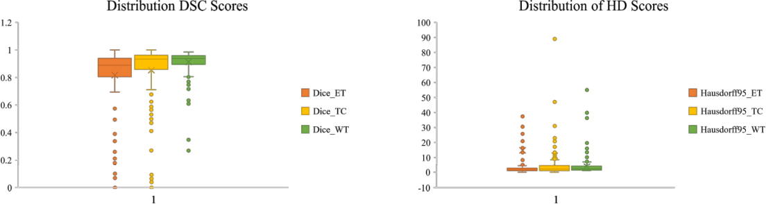
The quantitative and qualitative results of online validation phase evaluation for the proposed approach is shown in Table 1 Fig. 4 and Fig. 3.
 |
 |
4 Conclusion
We proposed a Transformer-based method that has adapted two windowing strategies in encoder to extract the long-range dependencies both within and across different modalities of mpMRI. We validated our method on brain tumor segmentation using FeTS Challenge 2022 dataset and results demonstrate the effectiveness of the proposed method.
References
- [1] Baid, U., Ghodasara, S., Bilello, M., Mohan, S., Calabrese, E., Colak, E., Farahani, K., Kalpathy-Cramer, J., Kitamura, F.C., Pati, S., et al.: The rsna-asnr-miccai brats 2021 benchmark on brain tumor segmentation and radiogenomic classification. arXiv preprint arXiv:2107.02314 (2021)
- [2] Cao, H., Wang, Y., Chen, J., Jiang, D., Zhang, X., Tian, Q., Wang, M.: Swin-unet: Unet-like pure transformer for medical image segmentation. arXiv preprint arXiv:2105.05537 (2021)
- [3] Çiçek, Ö., Abdulkadir, A., Lienkamp, S.S., Brox, T., Ronneberger, O.: 3d u-net: learning dense volumetric segmentation from sparse annotation. In: International conference on medical image computing and computer-assisted intervention. pp. 424–432. Springer (2016)
- [4] Dong, X., Bao, J., Chen, D., Zhang, W., Yu, N., Yuan, L., Chen, D., Guo, B.: Cswin transformer: A general vision transformer backbone with cross-shaped windows. arXiv preprint arXiv:2107.00652 (2021)
- [5] Dosovitskiy, A., Beyer, L., Kolesnikov, A., Weissenborn, D., Zhai, X., Unterthiner, T., Dehghani, M., Minderer, M., Heigold, G., Gelly, S., et al.: An image is worth 16x16 words: Transformers for image recognition at scale. arXiv preprint arXiv:2010.11929 (2020)
- [6] Hatamizadeh, A., Tang, Y., Nath, V., Yang, D., Myronenko, A., Landman, B., Roth, H.R., Xu, D.: Unetr: Transformers for 3d medical image segmentation. In: Proceedings of the IEEE/CVF Winter Conference on Applications of Computer Vision. pp. 574–584 (2022)
- [7] Liu, Z., Lin, Y., Cao, Y., Hu, H., Wei, Y., Zhang, Z., Lin, S., Guo, B.: Swin transformer: Hierarchical vision transformer using shifted windows. arXiv preprint arXiv:2103.14030 (2021)
- [8] Luu, H.M., Park, S.H.: Extending nn-unet for brain tumor segmentation. arXiv preprint arXiv:2112.04653 (2021)
- [9] Miyato, T., Maeda, S.i., Koyama, M., Ishii, S.: Virtual adversarial training: a regularization method for supervised and semi-supervised learning 41(8), 1979–1993 (2018)
- [10] Naseer, M., Ranasinghe, K., Khan, S., Hayat, M., Khan, F.S., Yang, M.H.: Intriguing properties of vision transformers. arXiv preprint arXiv:2105.10497 (2021)
- [11] Pati, S., Baid, U., Zenk, M., Edwards, B., Sheller, M., Reina, G.A., Foley, P., Gruzdev, A., Martin, J., Albarqouni, S., et al.: The federated tumor segmentation (fets) challenge. arXiv preprint arXiv:2105.05874 (2021)
- [12] Peiris, H., Chen, Z., Egan, G., Harandi, M.: Reciprocal adversarial learning for brain tumor segmentation: a solution to brats challenge 2021 segmentation task. arXiv preprint arXiv:2201.03777 (2022)
- [13] Peiris, H., Hayat, M., Chen, Z., Egan, G., Harandi, M.: A volumetric transformer for accurate 3d tumor segmentation. arXiv preprint arXiv:2111.13300 (2021)
- [14] Reina, G.A., Gruzdev, A., Foley, P., Perepelkina, O., Sharma, M., Davidyuk, I., Trushkin, I., Radionov, M., Mokrov, A., Agapov, D., et al.: Openfl: An open-source framework for federated learning. arXiv preprint arXiv:2105.06413 (2021)
- [15] Ronneberger, O., Fischer, P., Brox, T.: U-net: Convolutional networks for biomedical image segmentation. In: MICCAI. pp. 234–241. Springer (2015)
- [16] Sheller, M.J., Edwards, B., Reina, G.A., Martin, J., Pati, S., Kotrotsou, A., Milchenko, M., Xu, W., Marcus, D., Colen, R.R., et al.: Federated learning in medicine: facilitating multi-institutional collaborations without sharing patient data. Scientific reports 10(1), 1–12 (2020)
- [17] Vaswani, A., Shazeer, N., Parmar, N., Uszkoreit, J., Jones, L., Gomez, A.N., Kaiser, Ł., Polosukhin, I.: Attention is all you need. In: Advances in neural information processing systems. pp. 5998–6008 (2017)
- [18] Wang, W., Chen, C., Ding, M., Yu, H., Zha, S., Li, J.: Transbts: Multimodal brain tumor segmentation using transformer. In: International Conference on Medical Image Computing and Computer-Assisted Intervention. pp. 109–119. Springer (2021)
- [19] Wu, W., Chen, A.Y., Zhao, L., Corso, J.J.: Brain tumor detection and segmentation in a crf (conditional random fields) framework with pixel-pairwise affinity and superpixel-level features. International journal of computer assisted radiology and surgery 9(2), 241–253 (2014)
- [20] Zhou, H.Y., Guo, J., Zhang, Y., Yu, L., Wang, L., Yu, Y.: nnformer: Interleaved transformer for volumetric segmentation. arXiv preprint arXiv:2109.03201 (2021)
- [21] Zikic, D., Glocker, B., Konukoglu, E., Criminisi, A., Demiralp, C., Shotton, J., Thomas, O.M., Das, T., Jena, R., Price, S.J.: Decision forests for tissue-specific segmentation of high-grade gliomas in multi-channel mr. In: International Conference on Medical Image Computing and Computer-Assisted Intervention. pp. 369–376. Springer (2012)