Existence of Partially Quadratic Lyapunov Functions That Can Certify The Local Asymptotic Stability of Nonlinear Systems
Abstract
This paper proposes a method for certifying the local asymptotic stability of a given nonlinear Ordinary Differential Equation (ODE) by using Sum-of-Squares (SOS) programming to search for a partially quadratic Lyapunov Function (LF). The proposed method is particularly well suited to the stability analysis of ODEs with high dimensional state spaces. This is due to the fact that partially quadratic LFs are parametrized by fewer decision variables when compared with general SOS LFs. The main contribution of this paper is using the Center Manifold Theorem to show that partially quadratic LFs that certify the local asymptotic stability of a given ODE exist under certain conditions.
I Introduction
There is an abundance and diversity of applications found throughout science where a dynamical system is modelled as a nonlinear Ordinary Differential Equation (ODE). ODEs are at the core of many topics ranging from chaos theory, with the Lorenz equation [1], population dynamics [2], power systems [3] and many more. Understanding the long term properties of solutions to general ODEs is therefore of critical importance. Arguably the most fundamental and sort after long term property is that of local stability. A system described by an ODE is said to be locally asymptotically stable if solutions initialized near an equilibrium point remain near this equilibrium point for all time and furthermore converge towards this equilibrium point as time increases.
This paper considers the following problem: Given an ODE and its equilibrium point, certify whether or not this ODE is locally asymptotically stable. To solve this problem we take the approach that is perhaps the most universally used technique, Lyapunov’s second method. This method certifies the stability of ODEs by finding a function satisfying certain properties called a Lyapunov Function (LF).
A common approach to numerically searching for LFs has been to use Sum-of-Square (SOS) programming [4]. Unfortunately, searching for SOS LFs is known to scale poorly with respect to the state space dimension of the system [5]. One approach to improving the scalability of SOS has been to decompose large scale systems into lower dimensional subsystems. Several methods exist that show that if a suitable decomposition can be found then the stability of the lower dimensional subsystems imply the stability of the original large scale system [6, 7, 8]. Unfortunately, these methods often lack generality assuming that the system has a certain structure that allows for such decompositions.
Recently there has been significant interest in improving the scalability of SOS methods by searching for “separable” or “structured” LFs of the form,
Such separable LFs can be found in the works of [9, 10, 11] and in the related reachable set computation problems [12, 13]. These works demonstrate that searching for “structured” LFs improve numerical performance. It has been shown in [14] that monotone systems over compact state spaces posses max-separable LFs. However, in general, it is unknown for what class systems possess such “structured” LFs.
Inspired by the works of [15, 16] that use the Center Manifold Theorem to construct converse LFs with certain structure, in this paper we propose a new approach for certifying the local asymptotic stability of general high state space nonlinear ODEs by searching for partially quadratic LFs of the form,
where , , and . Such LFs are partially quadratic since a subset of the state space variables, , appear in with degree at most two. The main contribution of this paper is to provide several conditions under which it can be shown that partially quadratic LFs exist.
II Notation
We denote a ball with radius centred at the origin by . Let be the space of continuous functions with domain and image . We denote the set of differentiable functions by . For we denote as the matrix function such that . For and we denote to be the vector of monomial basis in -dimensions with maximum degree . We denote the space of scalar valued polynomials with degree at most by . We say is a Sum-of-Squares (SOS) polynomial if there exists such that . We denote to be the set of -degree SOS polynomials.
III ODEs and Solution Maps
Consider a nonlinear Ordinary Differential Equation (ODE) of the form
| (1) |
where is the vector field. Note that, throughout this paper we will assume , implying the origin is an equilibrium point of the ODE (1).
The Solution Map of ODEs
Given , and we say any function satisfying
| (2) |
is a solution map of the ODE (1) over . For simplicity throughout the paper we will assume there exists a unique solution map to the ODE (1) over all . Note, if the vector field, , is Lipschitz continuous then the solution map exists for some finite time interval, furthermore, this finite time interval can be arbitrarily extended if the solution map does not leave some compact set, see [15].
Stability of Nonlinear ODEs
We now use the solution map of the ODE (1) to define several notions of stability.
Definition 1:
The equilibrium point of ODE (1) is,
- •
Stable if, for each , there exists such that
- •
Asymptotically stable if it is stable and there exists such that
- •
Exponentially stable if there exists such that
Given an ODE, if origin is an asymptotically stable equilibrium point of the ODE then we will say that the ODE is locally asymptotically stable.
Certifying the Stability of Nonlinear ODEs
In general there is no analytical expression for the solution map of a nonlinear ODE. Hence, directly certifying whether a nonlinear ODE is locally asymptotically stable by first finding the solution map, and then showing over some set is challenging. Fortunately, there exists several methods that can certify the local asymptotic stability of an ODE without first finding the solution map. Arguably, the most important of these methods, that we now state next, are Lyapunov’s first and second methods.
Lemma 1 (Lyapunov’s First Method):
Consider an ODE (1) defined by some vector field with . Let
| (3) |
It follows that,
- •
If all the real parts of the eigenvalues of are negative then the ODE is locally asymptotically stable.
- •
If there exists an eigenvalue of whose real part is positive then the ODE is not locally asymptotically stable.
From Lem. 1 we see that in the case when , given in Eq. (3), has an eigenvalue that is purely imaginative we are unable to use Lyapunov’s first method to certify whether the associated ODE is locally asymptotically stable or not. For this case we can still certify local asymptotic stability using Lyapunov’s Second Method, stated next.
Theorem 1 (Lyapunov’s Second Method [17]):
Consider an ODE (1) defined by some with . The ODE is locally asymptomatically stable if and only if there exists and that satisfies,
| (4) | ||||
| (5) |
In the special case of asymptotically stable linear systems, , it is well known that there exists a quadratic LF, where , and the Lyapunov condition of Thm. 1 reduces to the Matrix Equation (6) as shown in the next theorem.
Theorem 2 ([18]):
For any symmetric positive definite matrix , the Lyapunov matrix equation,
| (6) |
has a unique symmetric positive definite solution if every eigenvalue of has strictly negative real part.
Coordinate changes for block diagonalization of linearization matrix
In order to state the main result in Thm. 3, that there exists a converse partially quadratic LF, we must first make a coordinate change to the ODE (1). This coordinate change will allow us to write the ODE as two coupled ODEs whose state variables will either appear quadratically or non-quadratically in our converse LF.
Since we are concerned with certifying whether the ODE (1) is locally stable, WLOG, we now assume that the associated linearization matrix, , given in Eq. (3), has purely imaginary eigenvalues and that the remaining eigenvalues of have negative real parts. We assume this WLOG because in the case where all of the eigenvalues of have negative real parts (i.e ) we can certify that the ODE is locally stable by Lem. 1. Alternatively, if any of the eigenvalues of have positive real part then by Lem. 1 we can certify that the ODE is not locally asymptotically stable. In both of these cases there would be no need to find a LF.
Now, for a matrix, , that has eigenvalues that are either purely imaginary or have negative real parts, Lemma 3 (found in the Appendix) shows that there exists an invertible matrix for which
| (7) |
where has only purely imaginary eigenvalues and has eigenvalues with only negative real part.
Note that for any vector field with associated linearization matrix, , given in Eq. (3), it follows that , where is such that . Thus given an ODE (1), defined by a vector field , WLOG we assume for some function such that . Then, by making the coordinate change to ODE (1) we can consider the equivalent nonlinear ODE:
| (8) | ||||
| (9) |
where has purely imaginary eigenvalues, has eigenvalues with only negative real part, is such that for , is such that for , , is the algebraic multiplicity of eigenvalue , and is the set of distinct eigenvalues of with zero real part.
IV Converse Partially Quadratic LFs
We now use the Center Manifold Theorem (Thm. 4 found in the Appendix) to prove the main result of the paper, Thm. 3, that shows that under certain conditions there exists a partially quadratic LF. Before stating Thm. 3 we first give a preliminary result. This preliminary result shows that the conditions required in our main result are satisfied by some commonly encountered systems. Note that similar conditions appear in [19].
Lemma 2:
Consider an ODE (1) defined by a vector field . Suppose one or more of the following statements holds:
- •
The ODE is locally exponentially stable (Def. 1).
- •
The ODE is a gradient system. That is its vector field is of the form , where is some function that satisfies , for all and if and only if .
- •
The ODE is locally asymptotically stable with a one dimensional state space.
Then there exists a radius, , and a LF, , satisfying
| (10) | ||||
where and is such that .
Suppose the ODE is locally exponentially stable. Then by Corollary 77 from Page 245 in [20] there exists a LF that satisfies Eq. (10) with .
Next, suppose the ODE is a gradient system. Then satisfies Eq. (10) with .
Finally, suppose the ODE has state space dimension equal to one. By defining we see that the ODE is a gradient system. Hence, Eq. (10) is satisfied. ∎
We now show that for the ODE given in Eqs. (8) and (9) if Eq. (10) holds for the associated reduced ODE (30) then there exists a partially quadratic LF of the form given in Eq. (15) that can certify the local asymptotic stability of the ODE.
Theorem 3 (Existence of converse partially quadratic LFs):
Consider an ODE given by Eqs. (8) and (9) and the associated reduced ODE (30). Suppose there exists a function satisfying Eq. (10) for the vector field of the reduced ODE (30). Then, the ODE given by Eqs. (8) and (9) is locally asymptotically stable if and only if there exists a matrix , a scalar and functions and such that
| (11) |
and
| (12) | ||||
| (13) | ||||
| (14) | ||||
| (15) |
First suppose that there exists a matrix , a scalar and functions and such that Eqs. (11), (12), (13) and (14) hold, where is given by Eq. (15). Now, it follows that is a LF for the ODE given by Eqs. (8) and (9) and hence this ODE is locally asymptotically stable by Thm. 1.
On the other hand let us now suppose the ODE given by Eqs. (8) and (9) is locally asymptotically stable. Consider the following function,
where satisfies Eq. (10) for some radius and for the vector field of the reduced ODE (30), given by , where satisfies PDE (29) for some radius (known to exist by Thm. 4), and is such that
| (16) |
Note that such a exists by Thm. 2 since is defined in Eq. (9) to have eigenvalues with only negative real part.
Now, it clearly follows by multiplying out the quadratic terms in that,
| (17) |
Hence, satisfies Eq. (15) with and .
We next show that satisfies Eqs. (12) and (13). The function comprises of the sum of two positive terms and thus it is clear for all . Clearly if and only if both of these positive terms are zero. Now, if and only if and if and only if . If and then (note that by Theorem 4). Therefore if and only if .
We next show that satisfies Eq. (14). First note that and defined in Eqs. (8) and (9) are such that and . Then by Lem. 4 (found in the Appendix) it follows that for , where is the largest eigenvalue of , there exists such that
| (18) | ||||
The second equality from Eq. (19) follows from the application of PDE (29), found in Thm. 4 from the Appendix. The first inequality of Eq. (19) follows from Eqs. (10) and (16) and the Cauchy Schwarz inequality. The second inequality of Eq. (19) follows from Eq. (18). The third inequality of Eq. (19) using the inequality for all . The fourth and final inequality in Eq. (19) follows since and hence and .
Therefore it follows that , given in Eq. (17), satisfies Eqs. (12), (13) and (14) for . ∎If there exists a function satisfying Eq. (10) for the reduced ODE (30) then Thm. 3 shows that the ODE given in Eqs. (8) and (9) is locally asymptotically stable if and only if there exists a partially quadratic LF. Further to this Lem. 2 provides some sufficient conditions that guarantee the existence of such a function . In the next corollary we combine these results to show the existence of partially quadratic LFs for systems whose linearization matrix has only one purely imaginary eigenvalue. This corollary provides the theoretical justification for the search of partially quadratic LFs to certify local asymptotic stability in our numerical examples in Sec. VI.
Corollary 1:
Consider an ODE (1) with associated linearization matrix defined in Eq. (3). Suppose there is a single purely imaginary eigenvalue of and all other eigenvalues of have negative real parts. Then the ODE is stable if and only if there exists a partially quadratic LF of the form given in Eq. (15) that satisfies Eqs (12), (13) and (14).
Follows using Prop. 1, Lem. 2 and Thm. 1. ∎Note, the proof of the existence of partially quadratic LFs given in Thm. 3 is non-constructive, being based on the center manifold, , for which in general there is no analytical formula. In the special case where the center manifold is analytically known the proof becomes constructive. In the following illustrative example we use Eq. (17) to construct a partially quadratic LF without any computation. Later, in Sec. V we will consider high dimensional systems for which the center manifold is not known and hence such a LF cannot be constructively found. For such systems we will use numerical methods to search for partially quadratic LFs to certify local asymptotic stability.
An Illustrative Example
Consider the following ODE,
| (20) | ||||
The associated linearization matrix, found in Eq. (3), is given by . The matrix has eigenvalues and and thus ODE (20) cannot be certified as locally asymptotically stable using Lyapunov’s first method (Lem. 1).
Note that without any coordinate transformations ODE (20) is already in the form of ODE given by Eqs. (8) and (9) with and . Thus setting it follows that . It is shown in [21] that gives the center manifold. Hence, the reduced ODE (30) associated with ODE (20) is,
| (21) |
ODE (21) has a one dimensional state space so by Lem. 2 it follows that there exists a function satisfying Eq. (10). Specifically, if we let it can be shown satisfies Eq. (10) with . The proof of Thm. 3 then shows that the function given in Eq. (17) is a LF. For this ODE this then implies that the following function is a LF to ODE (20),
| (22) |
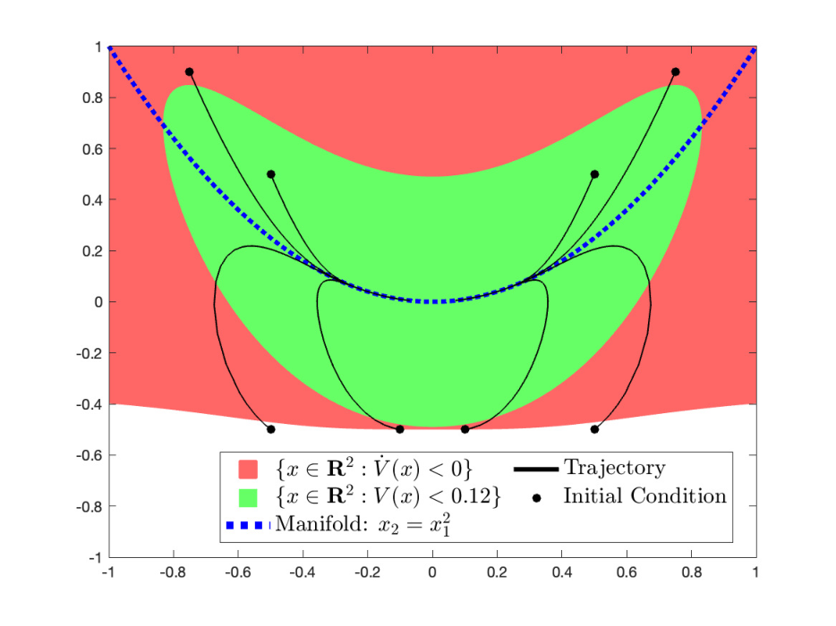
Clearly, the LF given in Eq. (22) is partially quadratic since the terms appear with degree at most while the terms can have degree greater . We have plotted the largest set of initial conditions that this LF can certify as asymptotically stable as the green region in Fig. 1(a).
V Using SOS to Certify Local Stability
Consider the problem of certifying the local stability of an ODE (1), defined by some vector field . This problem can be solved by using Lyapunov’s second method (Thm. 1). In cases where the vector field, , is polynomial we can search for such a LF using SOS programming [4, 22]. We can find such LFs by solving the following -degree SOS feasibility problem:
| (23) | ||||
where and . Note that is included in Opt. (23) so we only enforce to be a LF locally (over the ball ). Also note that is included in Opt. (23) to avoid the trivial solution . Typically and are selected to be small, for instance .
If ODE (1) is of the form given in Eqs. (8) and (9) then Thm. 3 indicates that we can certify local stability by searching for a partially quadratic LF of the form given in Eq. (15). This motivates the following -degree SOS feasibility problem:
| (24) | ||||
where , and .
Note, Opt. (24) can certify the local asymptotic stability of ODEs of the form given in Eqs. (8) and (9). General ODEs can be converted to be of this form using a coordinate change given in Eq. (7). This coordinate change can be numerically found using Matlab functions jordan and cdf2rdf.
Searching for partially quadratic LFs by solving Opt. (24) as opposed to searching for fully non-quadratic LFs by solving Opt. (23) results in computational savings due to the reduction in decision variables. These computational savings will be demonstrated through several numerical examples in the next section.
VI Numerical Examples
Example 1 (The Generalized Lotka–Volterra equations):
The competition of different groups (species, resources, etc) can be modelled by the following ODE,
| (25) | ||||
Clearly, ODE (25) has an equilibrium point at . The corresponding linearization matrix , given in Eq. (3), is such that Let us consider randomly generated values for and where and for all . Hence has eigenvalues which in this case are either purely imaginative or have negative real part. Thus we are unable to determine the stability of by Lyapunov’s first method. Cor. 1 shows this system is asymptotically stable iff there exists a partially quadratic LF. Solving Opts. (23) and (24) for to at , and , allows us to find feasible LFs in each case. In Fig. 1(b) we have plotted the difference in the number of decision variables associated with each optimization problem. For it took Yalmip [23] and Mosek 213s to solve Opt. (23) and 157s to solve Opt. (24).
Example 2 (Stable linear systems with nonlinear interconnection):
Let us consider the following ODE system,
| (26) | |||
where is such that and where all the eigenvalues of and have negative real part. The linearization matrix, given in Eq. (3), for this system is then This matrix is already in the block diagonal form of Eq. (7) with and . Since is one dimensional by Cor. 1 the system is locally asymptotically stable iff there exists a partially quadratic LF for this system.
For simplicity we will consider the case , and . For this ODE, , and we solve Opts. (23) and (24) for to , finding a LF in each case. Fig. 1(c) shows how the number of decision variables grows for each problem. For it took Yalmip [23] and Mosek 12645s to solve Opt. (23) and 10398s to solve Opt. (24).
VII Conclusion
We have proposed conditions for which there exists a partially quadratic LF that can certify the local asymptotic stability of nonlinear ODEs. The existence proof was non-constructive, relying on the existence of the center manifold. However, knowledge of the existence of partially quadratic LFs allows us to tighten our search of LFs, providing computational savings. This paper opens up many directions of future work such as investigating the conditions for which there exists a SOS partially quadratic LF and the conditions under which the proposed methods can be extended to global stability analysis.
References
- [1] Edward N Lorenz. Deterministic nonperiodic flow. Journal of atmospheric sciences, 20(2):130–141, 1963.
- [2] Vincent AA Jansen and Alun L Lloyd. Local stability analysis of spatially homogeneous solutions of multi-patch systems. Journal of mathematical biology, 41(3):232–252, 2000.
- [3] Lucas Lugnani, Morgan Jones, Luís F. C. Alberto, Mathew Peet, and Daniel Dotta. Combining trajectory data with energy functions for improved region of attraction estimation, 2021.
- [4] Declan Jagt, Sachin Shivakumar, Peter Seiler, and Matthew Peet. Efficient data structures for exploiting sparsity and structure in representation of polynomial optimization problems: Implementation in sostools, 2022.
- [5] Amir Ali Ahmadi and Anirudha Majumdar. Dsos and sdsos optimization: more tractable alternatives to sum of squares and semidefinite optimization. SIAM Journal on Applied Algebra and Geometry, 3(2):193–230, 2019.
- [6] Soumya Kundu and Marian Anghel. A sum-of-squares approach to the stability and control of interconnected systems using vector lyapunov functions. In 2015 American Control Conference (ACC), pages 5022–5028. IEEE, 2015.
- [7] James Anderson and Antonis Papachristodoulou. A decomposition technique for nonlinear dynamical system analysis. IEEE Transactions on Automatic Control, 57(6):1516–1521, 2011.
- [8] Corbinian Schlosser and Milan Korda. Sparse moment-sum-of-squares relaxations for nonlinear dynamical systems with guaranteed convergence. arXiv preprint arXiv:2012.05572, 2020.
- [9] Hiroshi Ito, Sergey Dashkovskiy, and Fabian Wirth. Capability and limitation of max-and sum-type construction of lyapunov functions for networks of iiss systems. Automatica, 48(6):1197–1204, 2012.
- [10] M Ali Al-Radhawi, David Angeli, and Eduardo D Sontag. A computational framework for a lyapunov-enabled analysis of biochemical reaction networks. PLoS computational biology, 16(2):e1007681, 2020.
- [11] Weehong Tan and Andrew Packard. Stability region analysis using polynomial and composite polynomial lyapunov functions and sum-of-squares programming. IEEE Transactions on Automatic Control, 53(2):565–571, 2008.
- [12] Matteo Tacchi, Carmen Cardozo, Didier Henrion, and Jean Bernard Lasserre. Approximating regions of attraction of a sparse polynomial differential system. IFAC-PapersOnLine, 53(2):3266–3271, 2020.
- [13] Vit Cibulka, Milan Korda, and Tomáš Haniš. Spatio-temporal decomposition of sum-of-squares programs for the region of attraction and reachability. IEEE Control Systems Letters, 6:812–817, 2021.
- [14] Anders Rantzer, Björn S Rüffer, and Gunther Dirr. Separable lyapunov functions for monotone systems. In 52nd IEEE Conference on Decision and Control, pages 4590–4594. IEEE, 2013.
- [15] H Khalil. Nonlinear Systems. 1996.
- [16] Bernard Haasdonk, Boumediene Hamzi, Gabriele Santin, and Dominik Wittwar. Kernel methods for center manifold approximation and a weak data-based version of the center manifold theorem. Physica D: Nonlinear Phenomena, 427:133007, 2021.
- [17] Andrea Bacciotti and Lionel Rosier. Liapunov functions and stability in control theory. Springer Science & Business Media, 2005.
- [18] Robert L Williams, Douglas A Lawrence, et al. Linear state-space control systems. John Wiley & Sons, 2007.
- [19] Ahmad N Atassi and Hassan K Khalil. A separation principle for the stabilization of a class of nonlinear systems. IEEE Transactions on Automatic Control, 44(9):1672–1687, 1999.
- [20] M. Vidyasagar. Nonlinear Systems Analysis: Second Edition. Classics in Applied Mathematics. Society for Industrial and Applied Mathematics (SIAM, 3600 Market Street, Floor 6, Philadelphia, PA 19104), 2002.
- [21] AJ Roberts. Low-dimensional modelling of dynamical systems. arXiv preprint chao-dyn/9705010, 1997.
- [22] James Anderson and Antonis Papachristodoulou. Advances in computational lyapunov analysis using sum of squares programming. Discrete and Continuous Dynamical Systems B, 20(8):2361–2381, 2015.
- [23] Johan Lofberg. Yalmip: A toolbox for modeling and optimization in matlab. In 2004 IEEE international conference on robotics and automation (IEEE Cat. No. 04CH37508), pages 284–289. IEEE, 2004.
- [24] Serge Lang. Linear algebra. Springer Science & Business Media, 1987.
Lemma 3:
Suppose the matrix has distinct eigenvalues for some . If sets are such that , , and if then for . Then there exists a non-singular matrix such that
where the set of eigenvalues of is equal to , the set of eigenvalues of is equal to , and is the algebraic multiplicity of eigenvalue .
Apply Theorem 4.2 Page 257 from [24]. ∎
Lemma 4:
Consider . Let . Then
| (27) |
Furthermore, if then for any there exists such that
| (28) |
By the Mean Value Theorem for any there exists such that
Then letting it follows that for all and . Hence, Eq. (27) follows.
Now suppose . Since it follows that , where . Then for any there exists such that for all . Thus it follows,
implying . Hence, Eq. (28) holds. ∎