FlexER: Flexible Entity Resolution for Multiple Intents (Technical Report)Conference: ; ;
Abstract.
Entity resolution, a longstanding problem of data cleaning and integration, aims at identifying data records that represent the same real-world entity. Existing approaches treat entity resolution as a universal task, assuming the existence of a single interpretation of a real-world entity and focusing only on finding matched records, separating corresponding from non-corresponding ones, with respect to this single interpretation. However, in real-world scenarios, where entity resolution is part of a more general data project, downstream applications may have varying interpretations of real-world entities relating, for example, to various user needs. In what follows, we introduce the problem of multiple intents entity resolution (MIER), an extension to the universal (single intent) entity resolution task. As a solution, we propose FlexER, utilizing contemporary solutions to universal entity resolution tasks to solve multiple intents entity resolution. FlexER addresses the problem as a multi-label classification problem. It combines intent-based representations of tuple pairs using a multiplex graph representation that serves as an input to a graph neural network (GNN). FlexER learns intent representations and improves the outcome to multiple resolution problems. A large-scale empirical evaluation introduces a new benchmark and, using also two well-known benchmarks, shows that FlexER effectively solves the MIER problem and outperforms the state-of-the-art for a universal entity resolution.
1. Introduction
An essential component of any data science lifecycle involves data preparation. Accordingly, contemporary data projects intensively invest in large-scale data cleaning and integration techniques to combine data from multiple heterogeneous sources into meaningful and valuable information. Consider, for example, a data-intensive organization (e.g., an online shopping company) that continuously collects data on user queries to better understand their needs. The (mostly implicit) intents of users may vary. While some users are interested in basketball shoes, regardless of their brand, others may be more interested in buying branded products, caring less whether shoes are designated as running shoes.
At the heart of the data preparation realm lies the entity resolution task (with variations of entity matching, record linkage, deduplication, and more), which has been extensively studied over the past decades (see books and surveys (Elmagarmid et al. 2006; Getoor and Machanavajjhala 2012; Christen 2012)). Entity resolution is a data integration task that aims at identifying same real-world entities that are represented by different data records (instances). Specifically, entity resolution can be used to “clean” a dataset from duplicate tuples referring to the same entity, offering a useful post processing tool for integrating multiple data sources.
Entity resolution techniques for resolving duplicates in a dataset were developed over years of research. Traditional methods focused on string similarity (Levenshtein 1966; Jaro 1989; Lin et al. 1998; Jaro 1995) and rule-based methods (Singla and Domingos 2006; Singh et al. 2017). Learning-based approaches were also suggested (Bilenko and Mooney 2003; Konda et al. 2016), followed by deep learning methods in recent years (Joty and Tang 2018; Mudgal et al. 2018; Fu et al. 2019; Kasai et al. 2019; Zhao and He 2019; Fu et al. 2020; Li et al. 2020b). Following a common practice for text processing, the use of pre-trained language models, and specifically, BERT-based models (Devlin et al. 2019), was also introduced for entity resolution (Li et al. 2020a; Brunner and Stockinger 2020; Li et al. 2021b; Peeters and Bizer 2021).
The aforementioned methods share a common assumption regarding the universality of the entity resolution problem, assuming the existence of a single interpretation to the notion of a real-world entity. In particular, most solutions aim to create a single clean view of a dataset, by separating corresponding from non-corresponding record pairs, with respect to this single interpretation.
The universal property of entity resolution solutions is being challenged by the development of applications that require the ability to provide a fine-grained (or personalized) analysis, offering services that are tailored to specific user needs and requirements (Yoganarasimhan 2019; Boratto and Marras 2021). For example, online shops aim at personalizing shopping experience to the needs of individual users, having to infer such needs from mainly implicit feedback (Kelly and Teevan 2003), such as clicks and mouse movements. In such a setting, having a universal resolution facility is likely to cripple the resolution process, failing to cater to the needs of all applications at all times. To illustrate the need for a non-universal (flexible) resolution, we use the AmazonMI dataset, a newly suggested benchmark based on amazon products data (see Section 5.1), in the following motivating example.
1.1. Motivating Example: From Record Duplication to Entity Resolution Interpretation
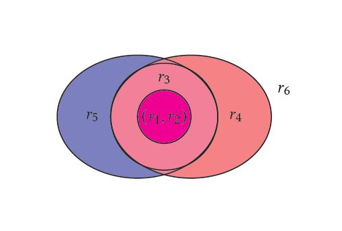
Table 1 depicts an excerpt of the AmazonMI dataset to illustrate the differences between the universal approach to entity resolution and the flexible entity resolution we present and address in this work. Figure 1 offers visual illustration to the multiplicity of entity interpretations in the example.
Record duplication is usually the result of discordant representations (e.g., multi-lingual, synonyms, capitalizations), changes in the data over time, typos, etc. For example, records and in Table 1 refer to the same pair of Nike basketball shoes called “Men’s Lunar Force 1 Duckboot.” The difference between and originates from capitalization issues (Nike vs. NIKE) and additional specification (e.g., color). Contrarily, and will most likely be conceived as different, as the latter refers to a book.
The pair () is an example of a pair that, under a certain interpretation, does not refer to the same entity, representing two different Nike basketball shoe variants. Yet, under a different interpretation, both and are Nike basketbsall shoes. Similarly, differs from and since they represent a different type of Nike shoes (basketball vs. running) and basketball shoes of different brands (Nike vs. Adidas), respectively, but may be determined to be representatives of the same entity (Nike shoes and basketball shoes, respectively) under a broader interpretation. Such different interpretation may be attributed to different user tastes or different contexts. For example, a pro basketball player would be more sensitive to differences between basketball shoes than a user that seeks shoes for a neighborhood afternoon fun game.
Over the years, entity resolution solutions resolved a single entity interpretation, detecting and as duplicates, to create a (single) clean dataset, e.g., by only preserving . The multiple intent phenomenon challenges any downstream application that requires entity matching and involves personalization to user’s needs. Beyond online shopping, multiple intents can be frequently found in the domain of recommendation systems, where user’s implicit feedback (e.g., item selection and search queries) can serve in understanding a user’s intent for better responding to her needs (Kelly and Teevan 2003).
| Product title | |
| Nike Men’s Lunar Force 1 Duckboot | |
| NIKE Men Lunar Force 1 Duckboot, | |
| Black/Dark Loden-BROGHT Crimson | |
| NIKE Men’s Air Max Stutter | |
| Step Ankle-High Basketball Shoe | |
| Nike Men’s Air Max 2016 Running Shoe | |
| adidas Performance Men’s | |
| D Rose 6 Boost Primeknit Basketball | |
| The Man Who Tried to Get Away |
1.2. Main Contributions
The motivating example offers an intuitive description of a scenario where a single dataset may serve as a basis for multiple clean views to be generated by an entity resolution solution, suggesting different interpretations of an entity in each such view. We use the term intent (formally defined in Section 2.2) to reflect user preferences that, in the scope of this paper, relate to the interpretation of the output view. We are, in particular, interested in intents that are unknown apriori and therefore cannot be constructed using data that exists in the database. Rather, such intents are known only through the training set that labels tuple pairs to be matched under a given interpretation. A typical such scenario can be found in recommendation systems where feedback is collected from users, either implicitly or explicitly, to be used to indicate intent. Another possible scenario may be motivated using machine learning algorithm for entity matching, where different tuning parameters yield different outcomes even for the same algorithm. For example, see the use-case of Yad VaShem, the Jewish Holocaust museum in Jerusalem (Sagi et al. 2016).
In this work, we define the problem of multiple intents entity resolution (MIER), an extension to the universal (single intent) entity resolution task. The MIER task considers multiple intents when creating a solution for potential downstream applications that involve entity resolution problems. In the absence of human interpretation to intents (recall the use of implicit feedback in recommendation systems to indicate intent), we aim at training a model to offer such interpretation based on training data and intent cross learning. We propose FlexER, a solution to the MIER problem that utilizes contemporary solutions to universal entity resolution tasks (e.g., DITTO (Li et al. 2020a)). FlexER positions the problem as a multi-label classification problem and combines intent-based representations of tuple pairs by creating an expressive multiplex graph. Graph neural network (GNN) uses the multiplex graph to learn latent relationships among intents, which in turn improves the outcome to multiple resolution problems. Our empirical evaluation uses two well-known benchmarks and proposes a new dataset for MIER, showing that FlexER provides accurate results for MIER. Moreover, FlexER outperforms state-of-the-art for the universal entity resolution problem. Specifically, the paper offers the following four contributions.
- (1)
A formulation of a new variation of the entity resolution problem, MIER, addressing the challenge of integrating and cleaning data in a multi-intent environment (Section 2.3).
- (2)
- (3)
A large-scale empirical evaluation showing the effectiveness of FlexER in solving MIER, while also outperforming the state-of-the-art on standard, universal entity resolution (Section 5).
- (4)
An open source access to FlexER implementation and the newly suggested benchmark dataset 11 1 https://github.com/BarGenossar/FlexER/.
2. Model and Problem Definiton
We present next an entity resolution model (Section 2.1) and introduce resolution intent (Section 2.2) as an extension to the universal entity resolution model to address multiple intents (Section 2.3). Table 2 summarizes the notations used throughout the following two sections.
| Notation | Meaning |
| Set of data records | |
| Set of entities | |
| Mapping from to | |
| Set of candidate record pairs | |
| A candidate pair in C | |
| Resolution | |
| Intent | |
| Set of intents | |
| The true label of with respect to intent | |
| The matcher prediction of with respect to intent |
2.1. (Single Intent) Entity Resolution
Entity resolution has several (analogous) definitions in the literature. We now present the model definition we use in this paper.
Let be a set of data records (dataset) and a set of real-world entities (). Each record is associated with an entity in using an entity mapping (mapping for short) . Whenever is unknown, for example, due to the absence of unique keys to identify entities, entity resolution solutions aim to pair records in such that if are paired together then . is usually characterized by a set of attributes , such that a record is assigned with values to all attributes (some of which may be null values). It is worth noting that in a data integration scenario where multiple data sources are involved, schema matching (Shraga et al. 2020) can provide an integrated attribute set and can be composed as a union of the sources.
Entity resolution is typically a three phase problem (see Figure 2). It starts with a blocking phase (Christen 2012), which aims to reduce the number of comparisons between records by eliminating record pairs for which . Such pairs can be deduced from the construction of . For example, in the case of a clean-clean resolution, where the integration task aims at integrating two clean data sources, each source is assumed to be duplicate-free by itself. Thus, two records that belong to the same data source cannot be matched together. Entity resolution solutions in the literature use the blocking phase as a tool to improve performance, by applying heuristics to assess the chance of and eliminating pairs that are unlikely to match. The blocking phase generates a set of candidate record pairs , over which matchers perform pairwise record pair comparisons.

During the matching phase, which is the focus of our work, a matcher assigns likelihood (similarity) scores to record pairs that endured the blocking phase. The likelihood score can be viewed as an estimation for the probability that . Applying a threshold over the likelihood scores yields , a resolution, containing record pairs that the matcher resolve to represent the same real-world entity. The relationship between resolution and entity mapping can be defined as follows.
Definition 0 (Resolution Satisfaction).
Let be a dataset, an entity set, , and an entity mapping. satisfies (denoted ) if , .
Finally, induced by the pairs in , the merging phase involves deriving , a clean view of , by choosing equivalence class representatives (Elmagarmid et al. 2006) (assuming reflexivity, symmetry, and transitivity).
Example 2.2.
Recall Table 1 (termed ) and let . Assume that some matcher assigns likelihood scores of to , to and a likelihood score lower than to all other record pairs in . Applying a threshold of , we obtain a resolution of , clustered into with a possible clean view .
Entity resolution matchers use similarity as a proxy to equivalence. Contemporary entity resolution solutions use learning-based matchers and typically cast the problem as a binary classification problem, classifying record pairs in a set as matched (equivalent) () or non-matched (). Record pair representation is the core ingredient of learning-based matchers. Prior art used multiple similarity scores (Konda et al. 2016), while recent works use record information (attribute values) to obtain a latent feature representation, based on individual representations (Joty and Tang 2018; Zhao and He 2019; Li et al. 2020b), attribute representations (Mudgal et al. 2018; Fu et al. 2019; Fu et al. 2020; Cappuzzo et al. 2020), or by creating a combined representation (Li et al. 2020a; Brunner and Stockinger 2020). Learning-based matchers typically assume the availability of a (labeled) training set to train a matcher, where denotes a record pair training set and if and otherwise.
Example 2.3 (DITTO Matcher).
DITTO (Li et al. 2020a) is an example of a deep learning-based state-of-the-art matcher for the entity resolution task. DITTO matches entities over candidate record pairs from two data sources and . DITTO serializes and tokenizes record pairs, adding a special token (termed ) to support classification (see (Devlin et al. 2019) for details). Then, it applies fine-tuning of a pre-trained transformer-based language (BERT-based) model to obtain latent representations (dimension of 768) for each tuple pair. These latent representations are used for binary classification using a linear layer. To enrich learning, DITTO injects domain knowledge, augments training data, and summarizes long strings.
2.2. Resolution Intents for Multiple Entity Interpretations
Standard resolution methods provide an adequate solution for universal entity resolution, a standalone task with a single interpretation (which we refer to as the equivalence intent). Yet, as motivated in Section 1.1, downstream data cleaning/integration applications may require different interpretations for the same input, to be formalized next as multiple resolution intents. We start with defining an intent.
Definition 0 (Resolution Intent).
Let be a dataset, an entity set and mapping from to . A resolution intent (intent for short) is a pair .
To better understand the meaning of multiple intents, we note that the universal view of entity resolution implicitly assumes a single entity set by which the entity resolution solution must abide. Such an entity set is not explicitly known, yet typically referred to abstractly as a “real-world entity." We argue that an entity set of choice may vary according to user needs, and that different users may seek different interpretations (and accordingly different solutions) for the same dataset. For illustration purposes, recall the motivating example (Section 1.1) demonstrating a case where users may seek varying entity interpretations. An attempt to seek a universal solution whenever multiple interpretations exist reduces the quality of the resolution outcome. For example, an intent to resolve and as matching records would fail under the universal entity resolution solution, which solely dictates .
We argue that the universal entity resolution has an underlying equivalence intent and assumes the existence of a single entity set and mapping such that if , then the records and refer to the same real world entity in (see Section 2.1). Entity resolution matchers, such as DITTO (see Example 2.3), all aim at solving the entity resolution problem with an equivalence intent. The framework that we suggest here takes into account resolution intent in the entity resolution process.
A mapping , while can be theoretically defined exhaustively, is pragmatically unknown. For ease of representation, we label intents using predicates such as “same category” or “same brand” when offering illustrating examples. Such labeling is for illustration purposes only and does not indicate that these predicates are known or can be derived from the data at hand. Rather, the model “perceives” the intents as sets of inputs (as explained in Example 2.3) and corresponding labels, and learns the underlying relationships between intents (to be explained in Section 4). We use to denote an intent.
Example 2.5.
Recall Table 1 with the dataset and let be an equivalence intent. We obtain under , using the subscript to relate the resolution with the intent description.
Let be an intent of “same brand.” Then, we obtain that all pairs are part of a resolution under . This means that the user having a intent, intends to resolve the records (Nike products). When looking at a “same category” intent , the resolution becomes less obvious. For example, , , , and share the same exact category (jointly representing basketball shoes). However, if we zoom out and look at the shoes category, a resolution satisfying the intent should also include . Such differences are reflected in the definition of intents, taking into account the overlap between categories. An additional intent may combine the two, referring to “same brand” and “same category,” to produce a resolution with record pairs (Nike basketball shoes). It is worth noting here that all intents are determined using the same input dataset.
2.3. Multiple Intents Entity Resolution (MIER)
Equipped with an intent definition as an entity set against which a mapping is computed, we next define the problem of multiple intents entity resolution (MIER). A MIER involves a set of (possibly related) entity mappings for a set of intents , offering multiple interpretations to resolve the entities in , each serving as a solution for a respective intent.
Problem 1 (Multiple Intents Entity Resolution).
Let be a dataset, and a set of intents.. A multiple intents entity resolution (MIER) seeks a set of resolutions over such that for each .
Intuitively, a solution for MIER should provide multiple solutions, each constituting a clean dataset view of for a different intent.
Example 2.6.
Recalling again our running example, now associated with a set of intents , a possible MIER solution over returns the resolutions , , , for the intents , , , and , respectively (illustrated in Figure 1). Out of these resolutions, we can generate the following clean views of , , , , (heuristically choosing representatives by order).
2.4. Intents Interrelationships
As illustrated in Example 2.5, intents are not simply standalone entity sets. Interrelationships among intents may provide useful hints on how to mix and match resolution results aiming to satisfy different intents. We begin with defining overlapping intents.
Definition 0 (Overlapping Intents).
Let be a dataset, , and two intents, where and are entity sets and and mappings from to and , respectively. are resolutions such that and . and overlap if .
For example, intents and overlap since the record pair is part of both resolutions.
In Section 4 we present our methodology to train a model to identify interrelationships among intents using multiplex graphs and a GNN. At times, it may be possible to identify special cases of overlapping intents. For example, consider subsumed intents, defined as follows.
Definition 0 (Subsumed Intents).
Let be a dataset, , and two intents, and resolutions such that and . is a sub-intent of if .
For example, is a sub-intent of . and are overlapping but not subsumed intents since, for example, is in but not in .
Subsumed intents may be the result of algorithm parameter tuning in a way that weakens the matching criteria so that the conditions of Definition 2.8 are met.
The resolution process can benefit from intents interrelationships. For example, having a resolution for an equivalence intent, we already know that all resolved record pairs with this intent will also be part of a resolution for a “same brand” intent, the former subsumed by the latter.
Whereas intents can be the outcome of inherent characteristics of the data (e.g., ontology, available attributes, etc.), they can also be formed according to user specifications. For intuition sake, recall Table 1 and assume the availability of sales data. The R&D department wishes to examine the impact a product’s store location has on its selling (e.g., how placing products of the same category but different brands in neighboring shelves contributes to the selling of the lower-price brand). In parallel, the purchasing department wants to determine the desired brand quantities to acquire. Although intents meaning by themselves are not necessarily unknown, interrelationships among them can be derived, either deterministically or stochastically. In this case, the R&D department focuses on category-level matching, while the purchasing department on brand-level matching. By receiving a set of candidate pairs with corresponding binary matching decisions of these intents, a machine learning model can derive, despite being agnostic to the intents’ underlying essence, that a match with respect to the latter intent implies a match with respect to the former.
3. Flexible Entity Resolution
As a preface to presenting our proposed solution, we first describe a general approach for addressing flexible entity resolution, entity resolution with more than one intent (Section 3.1). Then, we provide two baseline solutions to MIER. The first, termed in-parallel, treats multiple intents as a set of independent single intent problems. In this setting, each intent is considered individually and provides an independent solution for a single intent entity resolution (Section 3.2). An alternative approach, solving all intents jointly using multi-label learning, is presented in Section 3.3.
3.1. Entity Resolution Beyond a Single Intent
Just like other machine learning methods, learning-based matchers (e.g., DITTO, see Example 2.3), are trained (or fine-tuned) over a given set of training examples. In the context of universal single intent entity resolution (Section 2.1), a set of record pairs is labeled with respect to an equivalence intent (Section 2.2) to form a training set . Specifically, a record pair is labeled if the record pair satisfies .
Recalling that an intent induces a boolean space of record pairs, an entity resolution problem can be cast as a binary classification problem. Accordingly, a matcher22 2 We use the term matcher rather than classifier, noting that in the case of supervised learning these terms can be used interchangeably. aims to learn a resolution creation mapping , which separates record pairs that correspond () from those that do not (). Given an (unlabeled) test set of record pairs , the matcher classifies pairs, aiming for a resolution . In this setting, a Cross Entropy (CE) loss is used to train (fine-tune) the classifiers (Li et al. 2020a). Let and be the label and the likelihood score assigned by a matcher to , respectively. The cross entropy loss for the record pair is given by:
| (1) |
Similar to the way matchers learn to resolve a dataset under an equivalence intent, we can utilize the flexibility of learning-based matchers to learn other intents as well. Classifiers learn what we teach them. Thus, by using the same with different labels, we can train a matcher to resolve record pairs for any given intent. Therefore, given an intent , we can create a respective dataset , such that if the record pair satisfies , and otherwise.
3.2. Multiple Matchers For Multiple Intents
An in-parallel approach to MIER solves each intent separately, as illustrated in Figure 3. Specifically, an in-parallel approach transforms the multi-label problem into a set of binary problems, one for each label, as suggested by Read et al. (Read et al. 2011). This means that we solve each of the intents using separate training, yielding a different matcher and different record pair representations for each intent.

Given a set of intents (Section 2.2), we train binary matchers (one for each intent), where the matcher is responsible for creating a resolution to satisfy . We fine-tune each matcher independently using the CE loss (Eq. 1), i.e., , where is the likelihood score assigned by a matcher to according to the the ’th intent and is the label.
Given a (test) set of candidate pairs , a multi-label matcher returns binary labels as a solution for MIER. A set of resolutions is created with binary matchers , independently applying each .
3.3. Joint Learning of Multiple Intents
A possible disadvantage of an in-parallel solution is that intents are unaware of each other and the relationships between them are ignored. We now lay the groundwork for FlexER, aiming to jointly learn multiple intents. To do so, we treat the multi-label problem directly. The inherent assumption of this approach is that, since intents are interrelated, there exists some (latent) record pair representation (embedding) that can satisfy multiple intents simultaneously. This assumption, in fact, is also beneficial performance-wise. The in-parallel solution (Section 3.2) requires (the number of intents) separate training phases, whereas the multi-label solution requires a single, combined, training phase.

Given a set of intents , we create a multi-label dataset , such that is a binary label corresponding to the intent . Using the multi-label dataset, we train (fine-tune) a single multi-label matcher, , out of which we can also create a binary matcher for each intent, as illustrated in Figure 4.
Having a multi-label output, the standard cross entropy loss (Equation 1) does not capture the severity of an error per each head. For this reason, we replace it with a multi-label adaptation (Durand et al. 2019). Let and be the correct and predicted (likelihood scores) multi-label for , respectively. The loss for the record pair is given by:
| (2) | ||||
where is the function and is a weight, assigned to an error of the ’th intent.
To offer an intuition to the design choices of Eq. 2 we note that a multi-label problem is a generalization of multi class, where only a single class can be correct, i.e., . With multi-class classification, an extended version of the CE loss (Eq. 1) typically applies a transformation over the predictions representing a distribution over the classes to be the single correct class. With multiple intents, multiple classes can be labeled as true simultaneously. Therefore, instead of using , we apply a activation by element. To compensate for class (intent) imbalance, where some intents create bigger resolution sets (see Table 4 for imbalance illustration over the datasets in our experiments), intents can be assigned with different weights ().
Given a (test) candidate record pair from , we apply the trained resolution creation mappings over the intents to create a set of solutions out of which we can create a set of resolutions .
4. FlexER: Enhanced Resolution with Multiple Intents
Our proposed flexible entity resolution (FlexER) solution is a flexible approach to the MIER problem (Problem 1). FlexER zeros in on the matching phase, casting the problem as a multi-class multi-label task. FlexER builds upon the initial representations drawn from the in-parallel approach (Section 3.2) and extends the multi-label solution (see Section 3.3 and Figure 4), offering support to learning interrelationships among intents.
Recall that we target intents that are neither given explicitly nor known a-priori. They are not available as categories in the dataset and are not guided by human experts. Rather, they may be the outcome of occasional labeling following either explicit or implicit input of users. In particular, such labeling may follow different parameter tuning of algorithmic solutions to entity resolution that yields multiple interpretations of the data at hand. In such a setting, we argue that solving MIER requires a learning component to understand the interrelationships among intents as part of the main general task of yielding intent-level resolutions.
To obtain the maximum utility from record pair representations, FlexER makes use of an intents graph, a multiplex graph (Hamilton 2020) over record pair intent-based representations that codifies intents interrelationships (see Section 2.4). A multiplex graph is a special type of a multi-relational graph (Hamilton 2020), a graph with multiple edge types. Formally, a multi-relational graph is a triplet , where is a set of nodes, is a set of relation types and is a set of typed edges that connect pairs of nodes. An edge is a triplet, where and . Multiplex graphs are built in layers (see Figure 5, to be discussed in Section 4.1, for iilustration) and every node is duplicated in each of the layers. Each layer represents a unique concept and intra-layer edges correspond to relationships between nodes according to this concept. Nodes across different layers can be connected using inter-layer edges.
Multiplex graph allows an intuitive representation of a problem, of which the information regarding an object (node) is multi-faceted. Such graphs are prevalent in multi-dimensions systems like transportation networks and social networks. We design our intent graph as a multiplex graph, where a layer corresponds to an intent, and node in a layer corresponds to a record pair representation, according to that intent. The intent graph consists of node representation layers. We assign each record pair with a corresponding set of nodes , built upon initial representations drawn from the in-parallel approach (Section 3.2). Then, nodes referring to the same record pair are connected via intra-layer edges, whereas nodes within the same layer are connected through inter-layer edges to their closest record pair counterparts.
By applying a graph neural network (GNN) model over it, FlexER provides enriched intents-aware representations, which results in improved resolutions, yielding an intent-aware prediction for all record pairs. The entire process of FlexER involves three main phases, namely graph creation, message propagation, and prediction per intent, as detailed next.
4.1. Graph Creation
We begin with a brief description of generating intent-based representations, which are used to initialize the nodes of the graph, after which we discuss edge creation and labeling.

We use a pre-trained model and fine-tune it for each intent (intent-based representation). To support intent interrelationships, we enrich intent-based representations with the aid of other intent-based representations.
4.1.1. Nodes:
First, FlexER constructs a set of intent-layer nodes (see Figure 5 for an illustration of the constructed graph). These intent layers are initialized with the independent intent-based representation of all record pairs in a given set of candidate pairs , namely . In total, the number of nodes in the intents graph is .
We treat a node representation of a record pair as an initial feature vector, capturing the underlying semantics of the pair with respect to the task for which it was trained or tested against. Specifically, this task involves predicting whether a record pair matches a given intent. Node representations of the same pair for different intents are obtained independently, as the training process is carried out separately for each intent (see Section 3.2). As a result, node representations of different intent layers, while having the same dimensionality, belong to different latent spaces and their node representations are not aligned with each other, as the feature of each intent carries different meanings for the same record pair. Therefore, a main challenge here involves offering a meaningful way for pairs to update their initial representation by communicating with nodes at different layers.
4.1.2. Inter-Layer Edges:
To pave the way to intents-aware node representation, we define a set of inter-layer edges where . A set contains exactly edges, connecting a node from intent to its peer, the node representing the same record pair, of intent . These edges are utilized to propagate representation changes among layers. It is noteworthy that and are different and directionality of message propagation plays a key role in the next phase (Section 4.2). The total number of inter-layer edges is .
4.1.3. Intra-Layer Edges:
In addition to inter-layer edges, we also define , a set of intra-layer edges connecting a given node to its closest counterparts among the nodes of the same intent. This way, a pair representation can be enriched with those that are closely related to it for a specific intent. The intuition behind adding intra-layer edges comes from the nearest neighbor algorithm, where vector-space similarity is interpreted as agreement between samples (Bhatia et al. 2010). In Section 5.6 We empirically show that adding intra-layer edges improves FlexER’s performance.
We connect a node to its nearest neighbors, computed over an initial node representation. The identity of a node’s nearest neighbors may change during the iterative GNN process, yet the set of edges is predetermined and remains constant, which is in line with common good practices in GNN construction. The total number of generated intra-edges is . Note that intra-edges are directional. Therefore, while might be among the nearest neighbors of , the opposite does not necessarily hold.
4.1.4. Intent Graph as a Whole:
We illustrate the graph structure using Figure 5. In this example there are 11 record pairs, taken from Table 1. A pair in this figure is denoted by a node with the numbers of the two records it represents, and it appears in each of the given intent-layers. As portrayed by this figure, nodes can be spread differently in the space for different intents. Within a layer, a node is connected to its ( in this case) nearest neighbors with incoming edges. In addition, a node from one layer is connected to its peers from all other layers. For sake of ease of presentation, we present the inter-layer edges for the record pairs and only, and only between consecutive layers. We use a bidirectional edge to signify that two nodes are among the nearest neighbors of each other, e.g., pairs and for the Intent layer. When a record pair is a match according to a given intent, its underlying intent-layer node is marked with a dark color and white numbering, e.g., the pair for the Intent layer.
4.2. Message Propagation
The multiplex graph, whose generation is detailed in Section 4.1, lays the foundation to the usage of a GNN model as a mechanism to learn to characterize intents, as elaborated next. In what follows, it is worth noting that the term layer, as is being used in GNNs, refers to the pipeline of receiving messages from neighboring nodes, aggregating them, and applying a fully connected neural network with an activation function. For the intent graph, being a multiplex graph, a layer refers to a set of nodes of the same intent.
A general GNN architecture is composed of layers, each producing a hidden state vector, is generated by aggregating the vectors of adjacent nodes. Using the multi-layer GNN, each node iteratively transmits its current information to itself and its neighboring nodes (connected by outgoing edges). Numerous GNN models has been introduced in recent years. In this work, we follow the model of GraphSAGE (Hamilton et al. 2017) due to its popularity and ease of use.
The first hidden layer for the node , , is initialized to be the intent-based representation of the respective intent. In GraphSAGE, the update to the hidden state vectors at layer () of node is executed in two stages. First, neighbor messages are aggregated, yielding ’s neighborhood representation as follows.
| (3) |
where is an aggregation function (e.g., sum or mean) and is the set of ’s neighbors, connected by incoming edges. Then, this representation is concatenated to ’s previous layer representation, such that the resulted vector is fed into a fully connected neural network, followed by an activation function, as follows.
| (4) |
where is a vector concatenation operator, is an activation function (e.g., ReLU) applied in each layer except the last, and is the weights matrix of the -th convolution layer. We use a modified version of Eq. 3, adjusted for multiplex graphs. For more details we refer the interested reader to (Schlichtkrull et al. 2018).
4.3. Prediction per Intent
The final phase of training, after messages are propagated through the GNN, involves obtaining a prediction for each intent over all final hidden layers. FlexER is trained over versions of the same graph, one for each intent, to allow proper fine-tuning with respect to the target intent.
To provide a prediction for an intent , the final hidden representation of the node (), corresponding to the intent , is fed into a fully connected layer followed by a and an operations yielding the following:
| (5) |
where is the weights matrix of the fully connected layer and is a 2-dimensional prediction vector with entries corresponding to classes likelihood (its second entry, corresponding to the label , can be used as a likelihood score for , see Section 2.1). Given a record pair , is assigned with the entry ( or ) that has the highest likelihood, serving as the prediction for the intent .
5. Empirical Evaluation
We conducted a set of experiments to test FlexER’s ability to offer accurate resolutions and improve on single intent resolutions. We also evaluate the benefit of learning intents over intent graphs using a GNN architecture. We begin by describing the benchmarks (Section 5.1) and experimental setup (Section 5.2). Our main results, can be summarized as follows.
- •
FlexER effectively solves the task of MIER (Section 5.3).
- •
FlexER outperforms state-of-the-art baselines over all examined benchmarks for the entity resolution task (Section 5.4).
- •
FlexER benefits from inter-layer edges, making use of intent-based information to improve its performance for the task of universal entity resolution (Section 5.5).
- •
FlexER utilizes the component of intra-layer edges, such that connecting all nodes with other nodes from their own multiplex graph layer enhances the performance of the model over the task of universal entity resolution (Section 5.6).
5.1. Benchmarks and Intent Definition
We experimented with three benchmarks, among which a new publicly available benchmark for the MIER task (AmazonMI). In addition, we conducted experiments with a standard (clean-clean) entity matching benchmark (Walmart-Amazon) (Konda et al. 2016) and a product matching benchmark (WDC) (Primpeli et al. 2019). The datasets and their respective intent-based labels are provided in a git repository 33 3 https://github.com/BarGenossar/FlexER/tree/main/data/.
| Dataset | #Records | #Pairs | #Intents |
| () | () | () | |
| AmazonMI | |||
| Walmart-Amazon | |||
| WDC |
Metadata including cardinality of (#Records), (#Pairs), and number of intents (#Intents) is provided in Table 3. Table 4 presents the proportion of positive (matching) samples (%Pos) for each intent over the training, validation, and test sets.
| Dataset | Intent | %Pos | ||
| Train | Valid | Test | ||
| AmazonMI | (1) Eq. | 15.1% | 16.2% | 15.4% |
| (2) Brand | 20.0% | 21.3% | 21.4% | |
| (3) Set-Cat | 49.7% | 50.7% | 49.0% | |
| (4) Main-Cat. | 66.8% | 67.3% | 67.2% | |
| (5) Main-Cat. & | ||||
| Set-Cat. | 49.7% | 50.7% | 49.0% | |
| Walmart-Amazon | (1) Eq. | 9.4% | 9.4% | 9.4% |
| (2) Brand | 75.7% | 75.7% | 76.4% | |
| (3) Main-Cat. | 79.9% | 79.0% | 80.0% | |
| (4) General-Cat. | 89.7% | 90.2% | 90.5% | |
| WDC | (1) Eq. | 11.6% | 11.4% | 11.3% |
| (2) Cat. | 43.8% | 43.8% | 43.8% | |
| (3) General-Cat. | 67.0% | 66.6% | 67.2% | |
The datasets and corresponding intents are detailed next. All intents overlap (see Definition 2.7) and some are subsumed (see Definition 2.8). It is worth noting that Walmart-Amazon and WDC benchmarks are labeled solely for equivalence. Therefore, to support the empirical evaluation, we have created additional labeling using the provided data and known (to us but not the model) relationships between intents. Specifically, we ensure that labels according to a supersuming intent comply with subsumed intents.
The amazon multi intent benchmark (AmazonMI) consists of products, extracted from the amazon website. Product details include asin (unique identifier), title, brand, and an ordered category set. We only use product titles for matching, while other attributes (including the categories) are used for labeling only. To obtain the set of candidate pairs we use a standard blocker (Konda et al. 2016)44 4 https://github.com/anhaidgroup/py_entitymatching, preserving record pairs that share at least a 4-gram. We have created a ground truth of five intents for this benchmark, namely, equivalence (Eq.), same brand (Brand), same main-category (Main-Cat.), similar category-set (Set-Cat.), same main-category and similar category-set (Main-Cat. & Set-Cat.), as detailed next.
Tuple pairs were labeled according to the equivalence intent using an available online list of duplicated products 55 5 http://deepyeti.ucsd.edu/jianmo/amazon/metaFiles/duplicates.txt. For other intents we use the available product metadata. Pairs complying with the same brand intent (Brand) share a complete correspondence under the brand attribute. It is worth noting that during preprocessing, we defined the category of books as book and electronic books (Kindle) as Kindle, since those products did not have a brand value. The main-category (Main-Cat.) is defined as the first category in the (ordered) category-set provided by Amazon. The category-set reflects the product path in Amazon’s website; Hence, the first (main) category in the category-set depicts the most general affiliation of the product, wheres the last category is the most fine-grained. We define the intent of similar category set (Set-Cat.) as achieving a jaccard similarity of at least between the category-sets of a record in a pair. The last intent (Main-Cat. & Set-Cat.) satisfies both same main category and similar category set.
Walmart-Amazon 66 6 http://pages.cs.wisc.edu/~anhai/data1/deepmatcher_data/Structured/Walmart-Amazon/ matches entities of various product domains (Konda et al. 2016). We use the published pre-defined candidate pair sets provided in the literature as a basis for a ground truth of four intents. Similar to the AmazonMI dataset, the input of the model includes only the title, using other attributes for labeling intents. For this reason, the results we present for the equivalence (Section 5.4) intent cannot be directly compared with those reported in (Li et al. 2020a).
The intents used for Walmart-Amazon are equivalence (Eq.), same brand (Brand), same main category (Main-Cat.), and same general category (General-Cat.). The pairs were labeled as same brand if the two corresponding attribute values overlap. The creation of the category-based intents Main-Cat. and General-Cat. labels was not straightforward. Differences of category-tagging conventions between the two sources from which the data was taken (Walmart and Amazon) prevent direct comparison between tuples with respect to the category attribute. For example, for the matching tuples targus red tg-6660tr tripod with 3-way panhead and new-targus red tg-6660tr tripod with 3-way panhead 66 - meytg6660tr (only tuple titles are presented here), the category of the first tuple is photography - general, whereas the category of the second is tripods. Although these tuples match, the category of the first is more general than the second. To align between different category conventions, we manually created a hierarchical list of categories. The most general categories are electronics, personal equipment, house and cars. Other categories describe more specific concepts, e.g., computers is a subset of electronics. The full lists can be found in the git.77 7 https://github.com/BarGenossar/FlexER/
The web data commons (WDC) dataset 88 8 http://webdatacommons.org/largescaleproductcorpus/v2/index.html contains product data extracted from multiple e-shops, split into four categories, namely computers, cameras, watches, and shoes. Following (Li et al. 2020a), we only use product titles. For fair comparison, we use the pre-defined candidate pair sets, labeled for equivalence intent 99 9 https://github.com/megagonlabs/ditto/tree/master/data/wdc/all and use, to comply with other dataset sizes, the small size training set.
We define a category intent for this dataset, whose labels are obtained by the association to the relevant sub-datasets, each provided in a separate file.This structure creates a scenario where all pairs are labeled as matching (1) for the category intent within a provided category file. Thus, we expanded the dataset with cross-category pairs. To do so, we performed an additional blocking phase to generate additional non-matching pairs. For each pair of categories, we applied a blocker and pairs with a common 4-grams threshold (Konda et al. 2016) serve as cross-category, yet similar, tuple pairs. Out of these pairs, we randomly sampled pairs to be added to the original record pairs, yielding a new dataset with record pairs. We created an additional intent of general category by merging the computers and cameras categories into an electronics category, while watches and shoes were merged into a dressing category.
Finally, we randomly re-split the dataset into training, validation, and test subsets with the ratio of 3:1:1. Note that the original dataset contained total tuple pairs split into training, validation, and test set with sizes of , , and , respectively. This change affects our ability to reproduce the results reported in (Li et al. 2020a). The new version of the dataset in provided in the git repository 1010 10 https://github.com/BarGenossar/FlexER/tree/main/data/WDC/WDC_small.
Benchmarks Profiling: The AmazonMI forms a natural environment to the MIER problem, while the other two were modified to fit it. Recent works (Primpeli and Bizer 2020; Wang et al. 2021) focus on characterizing entity matching baselines, based on which we can derive insights regarding our expectations and room for improvements over these benchmarks (with respect to the equivalence intent). Primpeli et al. (Primpeli and Bizer 2020) defined a set of five profiling criteria, namely schema complexity (number of relevant attributes), textuality, sparsity (existence of null values), development size, and corner cases. Walmart-Amazon and WDC were already analyzed in this work, the former classified as textual with few corner cases, and the latter classified as textual with many corner cases group. Note that while we use a slightly different version of WDC this difference does not change the analysis. AmazonMI consists of a single attribute (title) with no null values. It contains long strings (>7 words) and low number of corner cases (<0.15). It is therefore classified as 1) dense data with simple schema, and 2) textual data with few corner cases. As pointed out by Primpeli et al. (Primpeli and Bizer 2020), these groups are expected to be relatively easy to solve; therefore, achieving a substantial improvement over existing baseline is challenging. We present in section 5.2.3 an evaluation measure (Eq. 7) which is aimed to asses the performance of a new model comparing to a given baseline in such cases.
5.2. Experimental Setup
Experiments were performed on a server with 2 Nvidia Quadro RTX 6000 and a CentOS 6.4 operating system. Networks were implemented using PyTorch (Paszke et al. 2019) and PyTorch Geometric (Fey and Lenssen 2019). The DITTO matcher (Li et al. 2020a) (see Example 2.3) was used to generate vector-based representations for all benchmarks, using RoBERTa (Liu et al. 2019) following (Li et al. 2020a). The complete code is available in a git.1111 11 http://github.com/BarGenossar/FlexER/
5.2.1. Implementation Details
We now provide implementation details for the central components in FlexER. We begin with describing the basic matching method (based on DITTO (Li et al. 2020a)), which is used as a preliminary step to create record pair representations, and continue with the graph creation, followed by intent interrelationships learning (using GNN).
DITTO: We adopted the implementation of DITTO (Li et al. 2020a) provided in publicly available code 1212 12 https://github.com/megagonlabs/ditto. Following (Li et al. 2020a), we set the input sequence to 512 tokens, the learning rate to , the number of epochs per run to , and use a batch size of 16. We tested three optimizations (Li et al. 2020a), namely data augmentation with the option of deleting spans of tokens, injecting domain knowledge on products, and data summarization to handle long input sequences, of which only the first yielded improved results. Therefore, we report only on the performance with data augmentation. Finally, we report the average performance over 5 different seeds. For the multi-label baseline (Section 3.3), we allocate an equal weight for each intent, after preliminary experiments showed no significant difference between this simple heuristic to parameters learning.
Multiplex Graph: Tuple pair representations serve in generating a multiplex graph that captures intent interrelationships. We employed vector-space similarity search using Faiss (Johnson et al. 2019) to connect each node to its nearest neighbors using distance. We tested and report on possible values (). For some of the experiments, we report only on the value that achieved the best performance over the validation set.
GNN: We enrich intent-based tuple pair representations, for better inference, using GNN that learns the interactions between intents (Section 4). We experimented with two or three layers of GraphSAGE (Hamilton et al. 2017), noting that more layers slowed down the training without enhancing performance. We trained the model over 150 epochs using Adam optimizer (Kingma and Ba 2014) with learning rate of , weight decay of and cross entropy loss function. We perform the hidden layer update (see Eq. 4) with ReLU activation function. In our experiments we examined several dimensions within the set , while for three-layer model the dimensionality is set as half of . We select the best preforming model over the validation set, and report the results over the test set.
5.2.2. Methodology
For each benchmark (Section 5.1), we first train a DITTO-based matcher/s. To generate independent intent-based representations, we train separate matchers, extracting for each an intent-based representation using the independent latent representations (see Example 2.3). For the multiple intent representation, we train a multi-task network, including a multi-label output and binary outputs (one per intent), using a single DITTO matcher. After fine-tuning the multi-task network, we extract the intent-based representations, using the latent representation of the layer prior to the output, per intent. These representations are used to construct the intent graph and the rest of the GNN inference (Section 4). In sections 5.3 and 5.4 we report on the results of FlexER using the independent intent-based representations.
5.2.3. Evaluation Measures
We evaluate the performance of entity resolution models over a single intent using the standard precision (P), recall (R), and F1 measure (F), as follows.
Let be a labeled set over a candidate record pair set for a single intent (see Section 3.2). The golden standard resolution over , such that , is given by . In addition, let be a resolution creating mapping over and its output, given by . Precision and recall are computed as follows:
| (6) |
The F1 measure, , is calculated as the harmonic mean of and . We use P, R, and F when the context is clear.
The state-of-the-art in entity resolution offers tools that perform extremely well over known benchmarks, especially for datasets that are profiled as easy (Primpeli and Bizer 2020) (see discussion in Section 5.1). We augment the standard measures by offering a refined analysis by measuring the % of baselines error that FlexER successfully removed. Given two resolutions (outcome of FlexER ) and (outcome of baseline), and an evaluation measure , where , the reduction of residual error is computed as follows:
| (7) |
To evaluate the quality of models for MIER, we use the average performance of the single intents per measure. Let be a set of intents and be the result with respect to intent . The multi intent performance (MI-V) is computed as
| (8) |
In addition, we measure multi label accuracy (Eq. 9). Let and be the -dimensional (a label for each intent) set of predicted and golden standard intent-based labels of , respectively. The multi label accuracy (-) over the candidate set is defined as follows.
| (9) |
where denotes an indicator function. We report on average over the tuple pairs in test set. Note that the is far more strict than , since it requires the multi intent matcher to be correct over all given intents.
Finally, to evaluate the importance of information propagation as a tool to utilize subsumption relationships, we use the measure preventable error of intent with respect to resolution and golden standard resolution , denoted as . This measure is defined as the ratio of false positive predictions that could be prevented by “listening” to at least one correct negative prediction of the intents which is subsumed by:
| (10) |
where is the set of false positive predictions in with respect to , and is the set of true negative predictions in , such that is the OR operator defined over the set of intents by which is subsumed.
5.2.4. Baselines
The baselines against which we compare FlexER solve either a MIER or a universal entity resolution problem.
Multi intent baseline: We use three baselines, as follows. A naïve baseline (Naïve) assumes that one-size-fits-all and hence, a single solution to the universal entity resolution problem can be applied to multiple intents. The other two baselines were presented in sections 3.2 (In-parallel) and 3.3 (Multi-label). We also report on the single intent performance using these methods.
Single intent baseline: We use the state-of-the-art (universal) entity resolution solution DITTO (Li et al. 2020a) (described in Example 2.3). Li et al. show that DITTO outperforms DeepMatcher (Mudgal et al. 2018) and follow up works (Fu et al. 2019; Kasai et al. 2019; Li et al. 2020b; Fu et al. 2020). Accordingly, we solely compare FlexER to DITTO and assume the latter superiority over former models. We report the re-produced results of DITTO (see Section 5.2.1) and note that they slightly differ from the ones reported in (Li et al. 2020a). Specifically, for WDC we modify the training/validation/test sets (see Section 5.1) and for Walmart-Amazon the differences may be attributed to the removal of two attributes (category and brand) to allow fair predictions over their underlying intents (see Section 5.1).
5.3. MIER
We first compare FlexER performance with the baseline methods in solving the MIER task. Table 5 compares the multi intent precision (), recall (), and F1 measure () (Eq. 8), multi intent accuracy (, Eq. 9) and multi intent reduction of residual error of F1 measure (, Eq. 7) of FlexER and a naïve, one-size-fits-all, approach (Naïve), the in-parallel approach (In-parallel, Section 3.2), and multi label learning (Multi-label, Section 3.3) over the three examined datasets (see Section 5.1).
| Dataset | Model | |||||
| AmazonMI | Naïve | .831 | .611 | .662 | .769 | - |
| In-parallel | .905 | .977 | .939 | .96 | - | |
| Multi-label | .856 | .975 | .907 | .931 | - | |
| FlexER | .951 | .976 | .964 | .977 | 41.0% | |
| Walmart- Amazon | Naïve | .933 | .282 | .350 | .437 | - |
| In-parallel | .924 | .918 | .921 | .932 | - | |
| Multi-label | .926 | .919 | .922 | .94 | - | |
| FlexER | .950 | .932 | .94 | .953 | 24.1% | |
| WDC | Naïve | .88 | .373 | .459 | .674 | - |
| In-parallel | .876 | .854 | .863 | .921 | - | |
| Multi-label | .881 | .836 | .857 | .914 | - | |
| FlexER | .871 | .872 | .871 | .922 | 5.8% |
As expected, the Naïve approach is unsuitable for the MIER task, resulting in very low recall values. Primarily, FlexER achieves the greatest improvement over the In-parallel baseline results for AmazonMI dataset, with average improvement of 2.7% and 1.8% in terms of and , respectively. These results reflect a reduction of residual error of () and (). Given that AmazonMI organically fits the characteristics of the multiple intent problem, we show that FlexER is well suited to solve MIER by enabling fruitful learning of intent interrelationships. As for Walmart-Amazon, MIER improves the results of the In-parallel baseline by 2.1% () and 2.3% (), namely 24.1% and 30.1% reduction of residual error. FlexER also achieves an improvement of 9.2% over the In-parallel baseline results for WDC dataset in terms of , albeit with a tiny improvement in terms of .
FlexER conjointly predicts accurate labels of different intents, as demonstrated by improvement. The naïve approach offers high precision and low recall, indicating that while a universal solution can provide an accurate resolution, it is also fairly small and incomplete with respect to other interpretations of the dataset.
5.4. Single Intent Entity Resolution
FlexER is designed to provide accurate resolutions for the MIER task (see Problem 1). We next demonstrate that FlexER can also improve single intent entity resolution, including the equivalence intent representing universal entity resolution (Section 5.4.1) and other intents (Section 5.4.2).
5.4.1. Equivalence Intent
Table 6 provides results in terms of precision (), recall (), F1 measure (), Accuracy () and (see Section 5.2.3) for equivalence intent solely, which is the universal entity resolution interpretation.
| Dataset | Model | |||||
| AmazonMI | In-parallel | .829 | .991 | .901 | .960 | - |
| Multi-label | .921 | .905 | .912 | .969 | - | |
| FlexER | .933 | .985 | .958 | .985 | 57.6 % | |
| Walmart- Amazon | In-parallel | .852 | .812 | .831 | .969 | - |
| Multi-label | .854 | .772 | .810 | .966 | - | |
| FlexER | .903 | .792 | .844 | .985 | 7.7 % | |
| WDC | In-parallel | .786 | .745 | .761 | .948 | - |
| Multi-label | .808 | .713 | .757 | .948 | - | |
| FlexER | .775 | .788 | .782 | .950 | 8.8 % |
Our experiments indicate that FlexER offers an improved performance of the equivalence intent (universal entity resolution). Compared to the state-of-the-art (DITTO), FlexER demonstrates a substantial increase of 6.3% for the AmazonMI dataset in terms of measure (reduction of residual error of 57.6%). FlexER also shows an improvement of 1.6% and 2.8% ( measure) compared to DITTO for the Walmart-Amazon and WDC dataset, respectively. These results indicate that with information of multiple intents annotations (e.g., derived from available meta data) FlexER is an effective solution for the universal entity resolution problem.
5.4.2. Other Intents
Table 7 provides results in terms of precision (), recall (), F1 measure (), Accuracy () and (see Section 5.2.3) for all datasets and their intents (except the equivalence intent that is reported in Table 6). We compare FlexER with the same baselines as in Section 5.4.1 for each single intent.
| Dataset | Intent | Model | Acc | ||||
| AmazonMI | Brand | DITTO (In-parallel) | .926 | .978 | .951 | .981 | - |
| Multi-label | .856 | .993 | .919 | .965 | - | ||
| FlexER | .934 | .979 | .956 | .982 | 10.2% | ||
| Set-Cat. | DITTO (In-parallel) | .912 | .977 | .944 | .944 | - | |
| Multi-label | .908 | .990 | .947 | .947 | - | ||
| FlexER | .968 | .976 | .972 | .973 | 50.0% | ||
| Main-Cat. | DITTO (In-parallel) | .979 | .989 | .984 | .978 | - | |
| Multi-label | .945 | .993 | .969 | .957 | - | ||
| FlexER | .988 | .987 | .988 | .983 | 25.0% | ||
| Main-Cat. + Set-Cat. | DITTO (In-parallel) | .881 | .948 | .913 | .937 | - | |
| Multi-label | .65 | .993 | .786 | .815 | - | ||
| FlexER | .932 | .955 | .944 | .961 | 35.6% | ||
| Walmart-Amazon | Brand | DITTO (In-parallel) | .977 | .964 | .971 | .955 | - |
| Multi-label | .970 | .976 | .973 | .959 | - | ||
| FlexER | .986 | .990 | .988 | .973 | 43.6% | ||
| Main-Cat. | DITTO (In-parallel) | .921 | .931 | .926 | .881 | - | |
| Multi-label | .927 | .952 | .939 | .901 | - | ||
| FlexER | .942 | .959 | .950 | .911 | 32.5% | ||
| General-Cat. | DITTO (In-parallel) | 0.948 | .968 | .957 | .922 | - | |
| Multi-label | .954 | .976 | .965 | .936 | - | ||
| FlexER | .967 | .987 | .977 | 945 | 46.5% | ||
| WDC | Category | DITTO (In-parallel) | .939 | .880 | .909 | .923 | - |
| Multi-label | .934 | .889 | .911 | .924 | - | ||
| FlexER | .932 | .89 | .911 | .923 | 1.0% | ||
| General-Cat. | DITTO (In-parallel) | .904 | .937 | .92 | .891 | - | |
| Multi-label | .902 | .905 | .904 | .870 | - | ||
| FlexER | .900 | .943 | .921 | .891 | 1.0% |
The results for AmazonMI demonstrates the ability of FlexER to benefit from intent interrelationships. The improvement achieved by FlexER over the intents of set-category and set-category+main-category is notably higher than the other two intents. The common thread between the two involves the subsumption relationship (Definition 2.8). set-category and set-category+main-category are subsumed by main-category. This implies that FlexER manages to propagates information among levels of granularity.
5.5. Inter-Layer Edge Analysis
In this subsection we examine the contribution of intents in solving universal entity resolution, and show that learning interconnections can help in avoiding preventable error (Eq. 10).
5.5.1. Intent Interrelationships


For each dataset we found the parameters (, and number of GNN layers) leading to the best average F1 value achieved over the universal entity resolution (equivalence intent), and fixed them. For each combination of these parameters, we generated the multiplex graph with every subset of the complete intent set which contains the equivalence intent. In addition, we also computed the average result over all possible k values () when remains fixed.
Figure 6 demonstrates the effectiveness of utilizing intent interrelationships, suggesting that in most cases the more is better. The numbers in the figure denote the intents according to their numbering in Table 4. For all datasets, the best result is achieved for the entire intent set, suggesting that FlexER benefits from additional information (more intents in our case) while solving the standard universal entity resolution task.
5.5.2. Intents Ablation Study
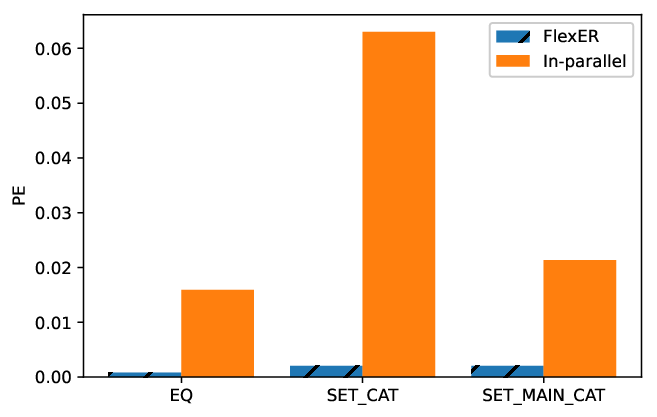
To measure the benefit of relying on intent interelationships, we use the measure of preventable error (Eq. 10), Focusing on AmazonMI and using the hyperparameters which lead to the best F1 score over the equivalence intent. Figure 7 demonstrates the gaps between FlexERand the in-parallel baseline in terms of this measure, as , while , which is approximately times more. This conclusion holds also for the set-category intent with , , and for the main-category+set-category intent with , . In both cases, we see an order of magnitude more preventable error.
Recall that real-world meaning of intents is unknown to the model. Therefore, relationships between intents cannot be directly derived. The above analysis reveals that FlexER offers an effective approach to learn those dependencies via a message propagation mechanism, significantly reducing the rate of preventable error.
5.6. Intra-Layer Edge Analysis
We tested FlexER’s performance using , and alongside the case of (no intra-layer edges) we report the average F1 value over all positive values for the universal entity resolution (equivalence intent). For these experiments we built the multiplex graph over the entire set of available intents.
| AmazonMI | Walmart-Amazon | WDC | |
| k=0 | .951 | .833 | .772 |
| k>0 | .955(+.42%) | .838(+.60%) | .777(+.65%) |
The experiment results are shown in Table 8, indicating that adding intra-layer edges is indeed effective. In both cases, the results obtained when are inferior to . Also, no clear dominance of a specific value is evident and the choice of remains a design choice that depends on the dataset. To summarize, the experiments strengthen the results presented in Section 5.5.2, as the results obtained by using the entire set of available intents are constantly better than the average values over all intent combinations containing the equivalence intent.
5.7. Run-Time Analysis
FlexER is built on top of intent-based representation, created by applying several DITTO models, one per intent. With adequate resources, those DITTO models can be trained simultaneously, such that considering multiple intent does not require extra time compared to an ordinary training of DITTO.
There are two modes of creating the multiplex graph. The first is performed exactly once for an entire hyperparamter set, including the nearest neighbors (NN) computation (Section 4.1.3). The second directly loads an available nearest neighbors dictionary, which can be done once the former mode is executed.
The run-times of FlexER over the three datasets (in seconds) are presented in Table 9. The nearest neighbors computation is orthogonal to the selection of hyperparameters. Hence, we separate the report of this calculation from the model training and testing. The reported run-times refer to the nearest neighbors computation of train, validation, and test dataset combined. It is not surprising that the size of the datasets directly affect this computation, as WDC requires significantly more time than the other two, while AmazonMI requires more time than Walmart-Amazon. Note that in our experiments we use only the exhaustive version of nearest neighbors computation, although Faiss (Johnson et al. 2019) offers multiple heuristics that can reduce the computational effort.
We also report on the run-time of the training and testing phase (over 150 epochs). While the hyperparameter selection of and does not drastically affect the run-times, we still report on average results over all examined combinations of these two. , the third hyperparameter, denotes the number of layers (2 or 3) in the GNN, which actually affects the training time. The results show that the burden of training and testing FlexERis negligible comparing to the preparatory phase of training DITTO model (approximately two orders of magnitude less). To conclude, once nearest neighbors dictionary is created, FlexER can be easily optimized over large set of hyperparameters due to its fast training time.
| AmazonMI | Walmart-Amazon | WDC | |
| NN Computation | 398.6 | 139.5 | 954.5 |
| Training+Testing(2L) | 11.4 | 8.1 | 6.7 |
| Training+Testing(3L) | 16.7 | 11.9 | 9.0 |
6. Related Work
Over the years, multiple solutions were suggested to tackle end-to-end entity resolution (Cohen and Richman 2002; Papadakis et al. 2020a) and its various steps (e.g., blocking (Papadakis et al. 2016; Papadakis et al. 2020b) and matching (Singh et al. 2017; Li et al. 2020a)). Overall, the main goal of entity resolution is to find equivalent record pairs, assuming that the more commonality they share the more similar they are (Lin et al. 1998). This observation has led to multiple similarity measure methods (Levenshtein 1966; Jaro 1989; Jaro 1995) that accurately estimate equality (Wang et al. 2011). More recent works aimed to improve such estimation by fusing similarity measures (Bilenko and Mooney 2003; Konda et al. 2016). Others aimed to extract rules from data for matching tuples (Singla and Domingos 2006; Singh et al. 2017), and recently even the usage of meta-learning techniques (Miao et al. 2021) was proposed. All of these methods address the universal entity resolution problem (Section 2.1), which, in the context of this paper, means resolving a single equivalence intent. We define and address the problem of MIER, extending universal entity resolution to support multiple resolution intents (including the equivalence intent). MIER is motivated by the need to support multiple entity interpretations in downstream applications. Our proposed solution, FlexER, is shown empirically to be backward compatible in that it offers an improved solution to the universal resolution intent as well.
Similar to other data integration tasks (Cappuzzo et al. 2020; Thirumuruganathan et al. 2020), deep learning is used to tackle entity resolution problems. Ebraheem et al. (Joty and Tang 2018) were the first to use neural networks for entity resolution, utilizing the contextual similarity of attribute values. Mudgal et al. (Mudgal et al. 2018) addressed the variation of entity matching by introducing a design space for the use of deep learning, which was later extended using multi-perspective matching (Fu et al. 2019), transfer learning (Kasai et al. 2019; Zhao and He 2019) and hierarchical network (Fu et al. 2020). Li et al. (Li et al. 2020b) use graph convolutional networks for the entity resolution task, albeit using a different representation of tuple pairs than ours.
The use of contextualized word embeddings based on pre-trained language models is beneficial in entity resolution (see (Li et al. 2021a; Brunner and Stockinger 2020; Li et al. 2020a)). Such models, and specifically BERT (Devlin et al. 2019), can cope with semantic heterogeneity in language and structural diversity in data instances. Studies (Li et al. 2020a; Brunner and Stockinger 2020) established the superiority of this approach over former methods by serializing input data to form a long string separated by artificial separator tokens, and fine-tuning a language model on top of the desired dataset. DITTO (Li et al. 2020a) enhances performance further using data augmentation, text summarization, and domain knowledge injection. DITTO is used in our work as a baseline, producing record pair representations (see Example 2.3).
Recent works (Li et al. 2021b; Peeters and Bizer 2021) suggest new variations of BERT-based structure architectures for entity resolution, allowing the network to train over a combination of more than a single loss function. Peeters et al. (Peeters et al. 2020) focus on product matching, a prevalent scenario of entity matching. They show that an intermediate training step over product datasets improves the effectiveness of BERT-based models to the task. The usage of pre-trained models is also extended to blocking (Thirumuruganathan et al. 2021). FlexER uses pre-trained models to address a new entity resolution problem, that of multiple intents (including equivalence), supported by graph convolutional networks, which also offers an improved solution to the universal entity resolution (equivalence intent) problem.
Several related works (Andritsos et al. 2006; Soliman et al. 2007; Dong et al. 2009) propose to examine multiple entity resolution problems (possible worlds) by attaching probabilities to resolutions/tuple pairs, to solve the universal entity resolution problem. Ensemble entity resolution approaches (Zhao and Ram 2005; Chen et al. 2009; Jurek et al. 2017; Meduri et al. 2020) combine multiple individual solutions to provide a more accurate single solution. FlexER solves a MIER problem, where different interpretations to the notion of a real-world entity lead to various intents with different solutions.
Recent works concentrate on leveraging external structure-based knowledge for extracting information. Karamanolakis et al. (Karamanolakis et al. 2020) focus on knowledge extraction using taxonomy with the objective of extracting category-specific attribute values based on the hierarchical structure of categories. Yu et al. (Yu et al. 2020) target expansion of taxonomy terms using natural supervision of existing taxonomies. Taxonomy is also shown to be valuable in the entity resolution pipeline, as part of the blocking phase (Wang et al. 2015), introducing a semantic similarity measure that relies on taxonomy trees. These works are distinct from ours. Whereas taxonomy-based frameworks start from a known taxonomy and make use of it, we do not assume intents structure is unknown. Rather, labels of training data are encoded in an intent graph, and a GNN is trained to recognize the mutual impact of intents.
7. Conclusions and Future Work
We presented MIER, an extension to the universal (single intent) entity resolution task, which caters to downstream applications that interpret resolutions in multiple ways. To tackle this problem, we introduce FlexER, utilizing contemporary solutions to universal entity resolution tasks to solve MIER. FlexER trains a graph neural network to learn intents through inter-intent relationships. To show the effectiveness of FlexER for MIER, we experimented with FlexER using three benchmarks, two adapted from existing entity resolution benchmarks along a new benchmark designed for MIER. We show that FlexER provides an improvement over the state-of-the-art baseline for the universal entity resolution task.
Future work include extensions of end-to-end entity resolution to support solving MIER. Specifically, we wish to test FlexER with additional matchers that produce record pair representations. In addition, we wish to investigate the role of blocking in MIER.
8. Acknowledgments
This work was supported in part by the National Science Foundation (NSF) under award numbers IIS- 1956096. We also acknowledge the support of the Benjamin and Florence Free Chair.
References
- (1)
- Andritsos et al. (2006) Periklis Andritsos, Ariel Fuxman, and Renee J Miller. 2006. Clean answers over dirty databases: A probabilistic approach. In 22nd International Conference on Data Engineering. IEEE, 30.
- Bhatia et al. (2010) Nitin Bhatia et al. 2010. Survey of nearest neighbor techniques. arXiv preprint arXiv:1007.0085 (2010).
- Bilenko and Mooney (2003) Mikhail Bilenko and Raymond J Mooney. 2003. Adaptive duplicate detection using learnable string similarity measures. In Proceedings of the ninth ACM SIGKDD international conference on Knowledge discovery and data mining. 39–48.
- Boratto and Marras (2021) Ludovico Boratto and Mirko Marras. 2021. Countering Bias in Personalized Rankings: From Data Engineering to Algorithm Development. In 2021 IEEE 37th International Conference on Data Engineering (ICDE). IEEE, 2362–2364.
- Brunner and Stockinger (2020) Ursin Brunner and Kurt Stockinger. 2020. Entity matching with transformer architectures-a step forward in data integration. In International Conference on Extending Database Technology.
- Cappuzzo et al. (2020) Riccardo Cappuzzo, Paolo Papotti, and Saravanan Thirumuruganathan. 2020. Creating embeddings of heterogeneous relational datasets for data integration tasks. In Proceedings of the 2020 ACM SIGMOD International Conference on Management of Data. 1335–1349.
- Chen et al. (2009) Zhaoqi Chen, Dmitri V Kalashnikov, and Sharad Mehrotra. 2009. Exploiting context analysis for combining multiple entity resolution systems. In Proceedings of the 2009 ACM SIGMOD International Conference on Management of data. 207–218.
- Christen (2012) Peter Christen. 2012. Data matching: concepts and techniques for record linkage, entity resolution, and duplicate detection. Springer Science & Business Media.
- Cohen and Richman (2002) William W Cohen and Jacob Richman. 2002. Learning to match and cluster large high-dimensional data sets for data integration. In Proceedings of the eighth ACM SIGKDD international conference on Knowledge discovery and data mining. 475–480.
- Devlin et al. (2019) Jacob Devlin, Ming-Wei Chang, Kenton Lee, and Kristina Toutanova. 2019. BERT: Pre-training of Deep Bidirectional Transformers for Language Understanding. In Proceedings of the 2019 Conference of the North American Chapter of the Association for Computational Linguistics: Human Language Technologies, Volume 1 (Long and Short Papers). 4171–4186.
- Dong et al. (2009) Xin Dong, Alon Halevy, and Cong Yu. 2009. Data integration with uncertainty. The VLDB Journal 18 (2009), 469–500.
- Durand et al. (2019) Thibaut Durand, Nazanin Mehrasa, and Greg Mori. 2019. Learning a deep convnet for multi-label classification with partial labels. In Proceedings of the IEEE/CVF Conference on Computer Vision and Pattern Recognition. 647–657.
- Elmagarmid et al. (2006) Ahmed K Elmagarmid, Panagiotis G Ipeirotis, and Vassilios S Verykios. 2006. Duplicate record detection: A survey. IEEE Transactions on knowledge and data engineering 19, 1 (2006), 1–16.
- Fey and Lenssen (2019) Matthias Fey and Jan Eric Lenssen. 2019. Fast graph representation learning with PyTorch Geometric. arXiv preprint arXiv:1903.02428 (2019).
- Fu et al. (2020) Cheng Fu, Xianpei Han, Jiaming He, and Le Sun. 2020. Hierarchical matching network for heterogeneous entity resolution. In Proceedings of the Twenty-Ninth International Joint Conference on Artificial Intelligence. 3665–3671.
- Fu et al. (2019) Cheng Fu, Xianpei Han, Le Sun, Bo Chen, Wei Zhang, Suhui Wu, and Hao Kong. 2019. End-to-End Multi-Perspective Matching for Entity Resolution.. In IJCAI. 4961–4967.
- Getoor and Machanavajjhala (2012) Lise Getoor and Ashwin Machanavajjhala. 2012. Entity resolution: theory, practice & open challenges. Proceedings of the VLDB Endowment 5, 12 (2012), 2018–2019.
- Hamilton et al. (2017) Will Hamilton, Zhitao Ying, and Jure Leskovec. 2017. Inductive representation learning on large graphs. Advances in neural information processing systems 30 (2017).
- Hamilton (2020) William L Hamilton. 2020. Graph representation learning. Synthesis Lectures on Artifical Intelligence and Machine Learning 14, 3 (2020), 1–159.
- Jaro (1989) Matthew A Jaro. 1989. Advances in record-linkage methodology as applied to matching the 1985 census of Tampa, Florida. J. Amer. Statist. Assoc. 84, 406 (1989), 414–420.
- Jaro (1995) Matthew A Jaro. 1995. Probabilistic linkage of large public health data files. Statistics in medicine 14, 5-7 (1995), 491–498.
- Johnson et al. (2019) Jeff Johnson, Matthijs Douze, and Hervé Jégou. 2019. Billion-scale similarity search with GPUs. IEEE Transactions on Big Data 7, 3 (2019), 535–547.
- Joty and Tang (2018) Muhammad Ebraheem Saravanan Thirumuruganathan Shafiq Joty and Mourad Ouzzani Nan Tang. 2018. Distributed Representations of Tuples for Entity Resolution. Proceedings of the VLDB Endowment 11, 11 (2018).
- Jurek et al. (2017) Anna Jurek, Jun Hong, Yuan Chi, and Weiru Liu. 2017. A novel ensemble learning approach to unsupervised record linkage. Information Systems 71 (2017), 40–54.
- Karamanolakis et al. (2020) Giannis Karamanolakis, Jun Ma, and Xin Luna Dong. 2020. Txtract: Taxonomy-aware knowledge extraction for thousands of product categories. arXiv preprint arXiv:2004.13852 (2020).
- Kasai et al. (2019) Jungo Kasai, Kun Qian, Sairam Gurajada, Yunyao Li, and Lucian Popa. 2019. Low-resource Deep Entity Resolution with Transfer and Active Learning. In Proceedings of the 57th Annual Meeting of the Association for Computational Linguistics. 5851–5861.
- Kelly and Teevan (2003) Diane Kelly and Jaime Teevan. 2003. Implicit feedback for inferring user preference: a bibliography. In Acm Sigir Forum, Vol. 37. ACM New York, NY, USA, 18–28.
- Kingma and Ba (2014) Diederik P Kingma and Jimmy Ba. 2014. Adam: A method for stochastic optimization. arXiv preprint arXiv:1412.6980 (2014).
- Konda et al. (2016) Pradap Konda et al. 2016. Magellan: Toward building entity matching management systems. Proceedings of the VLDB Endowment 9, 12 (2016), 1197–1208.
- Levenshtein (1966) Vladimir I Levenshtein. 1966. Binary codes capable of correcting deletions, insertions, and reversals. In Soviet physics doklady, Vol. 10. 707–710.
- Li et al. (2021b) Bing Li, Yukai Miao, Yaoshu Wang, Yifang Sun, and Wei Wang. 2021b. Improving the Efficiency and Effectiveness for BERT-based Entity Resolution.
- Li et al. (2020b) Bing Li, Wei Wang, Yifang Sun, Linhan Zhang, Muhammad Asif Ali, and Yi Wang. 2020b. GraphER: Token-Centric Entity Resolution with Graph Convolutional Neural Networks. In Proceedings of the AAAI Conference on Artificial Intelligence, Vol. 34. 8172–8179.
- Li et al. (2020a) Yuliang Li, Jinfeng Li, Yoshihiko Suhara, AnHai Doan, and Wang-Chiew Tan. 2020a. Deep entity matching with pre-trained language models. Proceedings of the VLDB Endowment 14, 1 (2020), 50–60.
- Li et al. (2021a) Yuliang Li, Jinfeng Li, Yoshihiko Suhara, Jin Wang, Wataru Hirota, and Wang-Chiew Tan. 2021a. Deep entity matching: Challenges and opportunities. Journal of Data and Information Quality (JDIQ) 13, 1 (2021), 1–17.
- Lin et al. (1998) Dekang Lin et al. 1998. An information-theoretic definition of similarity. In ICML, Vol. 98. 296–304.
- Liu et al. (2019) Yinhan Liu, Myle Ott, Naman Goyal, Jingfei Du, Mandar Joshi, Danqi Chen, Omer Levy, Mike Lewis, Luke Zettlemoyer, and Veselin Stoyanov. 2019. Roberta: A robustly optimized bert pretraining approach. arXiv preprint arXiv:1907.11692 (2019).
- Meduri et al. (2020) Venkata Vamsikrishna Meduri, Lucian Popa, Prithviraj Sen, and Mohamed Sarwat. 2020. A comprehensive benchmark framework for active learning methods in entity matching. In Proceedings of the 2020 ACM SIGMOD International Conference on Management of Data. 1133–1147.
- Miao et al. (2021) Zhengjie Miao, Yuliang Li, and Xiaolan Wang. 2021. Rotom: A meta-learned data augmentation framework for entity matching, data cleaning, text classification, and beyond. In Proceedings of the 2021 International Conference on Management of Data. 1303–1316.
- Mudgal et al. (2018) Sidharth Mudgal, Han Li, Theodoros Rekatsinas, AnHai Doan, Youngchoon Park, Ganesh Krishnan, Rohit Deep, Esteban Arcaute, and Vijay Raghavendra. 2018. Deep learning for entity matching: A design space exploration. In Proceedings of the 2018 International Conference on Management of Data. 19–34.
- Papadakis et al. (2020a) George Papadakis, George Mandilaras, Luca Gagliardelli, Giovanni Simonini, Emmanouil Thanos, George Giannakopoulos, Sonia Bergamaschi, Themis Palpanas, and Manolis Koubarakis. 2020a. Three-dimensional Entity Resolution with JedAI. Information Systems 93 (2020), 101565.
- Papadakis et al. (2020b) George Papadakis, Dimitrios Skoutas, Emmanouil Thanos, and Themis Palpanas. 2020b. Blocking and filtering techniques for entity resolution: A survey. ACM Computing Surveys (CSUR) 53, 2 (2020), 1–42.
- Papadakis et al. (2016) George Papadakis, Jonathan Svirsky, Avigdor Gal, and Themis Palpanas. 2016. Comparative analysis of approximate blocking techniques for entity resolution. Proceedings of the VLDB Endowment 9, 9 (2016), 684–695.
- Paszke et al. (2019) Adam Paszke, Sam Gross, Francisco Massa, Adam Lerer, James Bradbury, Gregory Chanan, Trevor Killeen, Zeming Lin, Natalia Gimelshein, Luca Antiga, et al. 2019. Pytorch: An imperative style, high-performance deep learning library. Advances in neural information processing systems 32 (2019).
- Peeters and Bizer (2021) Ralph Peeters and Christian Bizer. 2021. Dual-objective fine-tuning of BERT for entity matching. Proceedings of the VLDB Endowment 14, 10 (2021), 1913–1921.
- Peeters et al. (2020) Ralph Peeters, Christian Bizer, and Goran Glavaš. 2020. Intermediate training of BERT for product matching. small 745, 722 (2020), 2–112.
- Primpeli and Bizer (2020) Anna Primpeli and Christian Bizer. 2020. Profiling entity matching benchmark tasks. In Proceedings of the 29th ACM International Conference on Information & Knowledge Management. 3101–3108.
- Primpeli et al. (2019) Anna Primpeli, Ralph Peeters, and Christian Bizer. 2019. The WDC training dataset and gold standard for large-scale product matching. In Companion Proceedings of The 2019 World Wide Web Conference. 381–386.
- Read et al. (2011) J. Read, B. Pfahringer, G. Holmes, and E. Frank. 2011. Classifier chains for multi-label classification. Machine learning (2011).
- Sagi et al. (2016) Tomer Sagi, Avigdor Gal, Omer Barkol, Ruth Bergman, and Alexander Avram. 2016. Multi-Source Uncertain Entity Resolution at Yad Vashem: Transforming Holocaust Victim Reports into People. In Proceedings of the 2016 International Conference on Management of Data, SIGMOD Conference 2016, San Francisco, CA, USA, June 26 - July 01, 2016, Fatma Özcan, Georgia Koutrika, and Sam Madden (Eds.). ACM, 807–819. https://doi.org/10.1145/2882903.2903737
- Schlichtkrull et al. (2018) Michael Schlichtkrull, Thomas N Kipf, Peter Bloem, Rianne van den Berg, Ivan Titov, and Max Welling. 2018. Modeling relational data with graph convolutional networks. In European semantic web conference. Springer, 593–607.
- Shraga et al. (2020) Roee Shraga, Avigdor Gal, and Haggai Roitman. 2020. ADnEV: cross-domain schema matching using deep similarity matrix adjustment and evaluation. Proceedings of the VLDB Endowment 13, 9 (2020), 1401–1415.
- Singh et al. (2017) Rohit Singh, Venkata Vamsikrishna Meduri, Ahmed Elmagarmid, Samuel Madden, Paolo Papotti, Jorge-Arnulfo Quiané-Ruiz, Armando Solar-Lezama, and Nan Tang. 2017. Synthesizing entity matching rules by examples. Proceedings of the VLDB Endowment 11, 2 (2017), 189–202.
- Singla and Domingos (2006) Parag Singla and Pedro Domingos. 2006. Entity resolution with markov logic. In Sixth International Conference on Data Mining (ICDM’06). IEEE, 572–582.
- Soliman et al. (2007) Mohamed A Soliman, Ihab F Ilyas, and Kevin Chen-Chuan Chang. 2007. Top-k query processing in uncertain databases. In 2007 IEEE 23rd International Conference on Data Engineering. IEEE, 896–905.
- Thirumuruganathan et al. (2021) Saravanan Thirumuruganathan, Han Li, Nan Tang, Mourad Ouzzani, Yash Govind, Derek Paulsen, Glenn Fung, and AnHai Doan. 2021. Deep learning for blocking in entity matching: a design space exploration. Proceedings of the VLDB Endowment 14, 11 (2021), 2459–2472.
- Thirumuruganathan et al. (2020) Saravanan Thirumuruganathan, Nan Tang, Mourad Ouzzani, and AnHai Doan. 2020. Data Curation with Deep Learning.. In EDBT. 277–286.
- Wang et al. (2011) Jiannan Wang, Guoliang Li, Jeffrey Xu Yu, and Jianhua Feng. 2011. Entity matching: How similar is similar. Proceedings of the VLDB Endowment 4, 10 (2011), 622–633.
- Wang et al. (2021) Jin Wang, Yuliang Li, and Wataru Hirota. 2021. Machamp: A generalized entity matching benchmark. In Proceedings of the 30th ACM International Conference on Information & Knowledge Management. 4633–4642.
- Wang et al. (2015) Qing Wang, Mingyuan Cui, and Huizhi Liang. 2015. Semantic-aware blocking for entity resolution. IEEE Transactions on Knowledge and Data Engineering 28, 1 (2015), 166–180.
- Yoganarasimhan (2019) Hema Yoganarasimhan. 2019. Search personalization using machine learning. Management Science (2019).
- Yu et al. (2020) Yue Yu, Yinghao Li, Jiaming Shen, Hao Feng, Jimeng Sun, and Chao Zhang. 2020. STEAM: Self-Supervised Taxonomy Expansion with Mini-Paths. In Proceedings of the 26th ACM SIGKDD International Conference on Knowledge Discovery & Data Mining. 1026–1035.
- Zhao and He (2019) Chen Zhao and Yeye He. 2019. Auto-em: End-to-end fuzzy entity-matching using pre-trained deep models and transfer learning. In The World Wide Web Conference. 2413–2424.
- Zhao and Ram (2005) Huimin Zhao and Sudha Ram. 2005. Entity identification for heterogeneous database integration—a multiple classifier system approach and empirical evaluation. Information Systems 30, 2 (2005), 119–132.