Graph Neural Network Based Node Deployment
for Throughput Enhancement

Recently, network node deployment has been widely used to address the challenges of wireless communication networks, including congestion mitigation [13], coverage maximization [14], as well as quality-of-experience optimization [15]. Network node deployment has also been considered for throughput enhancement. In [5], the space is first divided into grids and then the network deployment is implemented with a brute force search method. In [6], a random geometry strategy based on the Poisson point process is developed to deploy the network nodes. In [7] and [8], uniform random deployment strategies are considered. Despite the simplicity of these deployment strategies in design, their performances are usually limited or suffer from intractable complexity.

For precise network deployment strategies, the requirement to find the exact locations of network nodes complicates the optimization problem. An analytical expression in [9] for the optimal location is derived by introducing the slack variables and leveraging the successive convex approximation. Based on the Lagrangian method, a dual problem for the approximate optimal solution is obtained in [10] by eliminating additional variables, which can be solved by a subgradient projection method. From a different viewpoint, the problem of maximizing the end-to-end throughput (i.e., max-flow) under jamming is considered in [11] and more recently in [12]. In both of these works, the max-flow was approximated by the Cheeger constant and its maximization was done by a spectral graph theoretical approach. Nevertheless, the approximations in these works may be loose and thus sometimes may lead to unsatisfactory performance.

The recently advocated GNN has a significant impact on wireless communications [16, 17], as many wireless networks can be naturally abstracted into graphs. In particular, GNNs have been widely applied to optimization problems in wireless communication networks [18, 19, 20], given the advantage that they can effectively utilize structural and topological information. These existing works mainly exploit permutation invariance and equivariance of GNNs to address the challenges in wireless communication networks. Besides, GNN can be embedded with deep reinforcement learning to enable sufficient exploration capabilities for graph-structural data in wireless communication networks. For instance, a solution to the connection management problem based on GNN and deep Q-Learning algorithm is proposed in [21], which achieved improvement in several objectives. In [22], a multi-agent PPO algorithm is proposed, which introduces the graph convolutional network with an empirically driven approach to training wireless MAC controllers. However, the problems considered in the above works are different from our research problem, and hence their solutions may not be directly applicable.

GNNs have been applied to representation learning on graphs since the seminal work of [23]. The important properties of permutation equivariance and invariance make GNNs suitable for graph data since they do not depend on a specific ordering of nodes [24, 25, 26, 27]. However, due to these invariance properties, GNNs are not expected to enjoy universal approximation [28]. In fact, GNNs are not sufficiently expressive for representing all permutation-invariant neural networks, and the equivalence between expressivity and approximation capability has been established in [29]. In particular, the Weisfeiler-Leman test is an important benchmark for the expressivity of GNNs and recent studies have focused on going beyond such limits [30, 31, 32]. The universality of a specific class of invariant/equivariant GNNs is proved in [26], relying on a new generalized Stone-Weierstrass theorem for the algebra of real-valued equivariant functions. The more general notion of universal approximation of group-invariant networks is studied in [33].

Many applications use the gradients of neural networks to approximate those of the original functions. An early study numerically studies training neural networks to approximate a multivariate function and its first and second partial derivatives [34]. When both function and gradient values are available, it is also possible to consider Sobolev training where the loss function is inherited from the Sobolev spaces [35, 36, 37]. However, Sobolev training is not applicable to our problem, since it is difficult to obtain precise gradients in our dataset.

In this work, we consider a wireless communication network with $n$ nodes, as shown in Fig. 1. The node deployment is denoted by $\left\{{\bm{\xi}}_{i}=\left(x_{i}^{\left(1\right)},x_{i}^{\left(2\right)}\right)\in\mathbb{R}^{2}:i=1,\dots,n\right\}$, where ${\bm{\xi}}_{1}$ and ${\bm{\xi}}_{n}$ are the locations of a pair of stationary source and destination nodes, and $\{{\bm{\xi}}_{i}\}_{i=2}^{n-1}$ are the locations of mobile relay nodes. With a slight abuse of notation, when there is no confusion, we may also use $\{{\bm{\xi}}_{i}\}_{i=1}^{n}$ to denote the nodes themselves. We model this wireless communication network using a simple graph ${\mathcal{G}}$ specified as follows. The vertex set of ${\mathcal{G}}$, denoted by ${\mathcal{V}}$, consists of all nodes $\{{\bm{\xi}}_{i}\}_{i=1}^{n}$. The edge set of ${\mathcal{G}}$, denoted by ${\mathcal{E}}$, consists of all pairs of nodes. We assume that for a pair of nodes ${\bm{\xi}}_{i}$ and ${\bm{\xi}}_{j}$, the corresponding communication rate between the pair of nodes is a function of their locations and is denoted by $f_{\rm cap}({\bm{\xi}}_{i},{\bm{\xi}}_{j})$. Moreover, we assume $f_{\rm cap}({\bm{\xi}}_{i},{\bm{\xi}}_{j})$ is a Lipschitz continuous function with respect to ${\bm{\xi}}_{i}$ and ${\bm{\xi}}_{j}$, which holds in most wireless scenarios. Accordingly, we construct the weighted adjacency matrix ${\bm{A}}$ of this network, whose $(i,j)$-th entry $A_{i,j}$ is defined as the communication rate between nodes $i$ and $j$. That is,

Our objective is to find the optimal locations of the relay nodes so that throughput (i.e., max-flow) between the source node and the destination node is optimized. It is well-known [38] that when the locations of the nodes are specified, this max-flow equals to the min-cut $C$ of the underlying network graph, defined by

where $S$ is a subset of ${\mathcal{V}}$, $\bar{S}$ is the complement of $S$, the minimum is taken over all partitions $\{S,\bar{S}\}$ of ${\mathcal{V}}$.

Clearly, the maximum network flow $C$ is a function of the edge weights $A_{i,j}$’s, and thus also a function of the locations ${\bm{\xi}}_{i}$ of the nodes. Actually, $C$ is a $1$-Lipschitz function with respect to each edge weight $A_{i,j}$. We state this fact as a lemma.

As a composition of Lipschitz functions, $C$ itself is Lipschitz with respect to the locations ${\bm{\xi}}_{i}$ of the nodes as well (see e.g., [39, Lemma 2.1]). Accordingly, Rademacher’s Theorem [40, Theorem 3.1.6] immediately yields the following result.

With the above notations, to optimize the throughput, we need to resolve the following problem.

We remark that this problem is permutation invariant. That is, if $({\bm{\xi}}_{2}^{*},\cdots,{\bm{\xi}}_{n-1}^{*})$ is an optimizer of (6), then its any permuted version $({\bm{\xi}}_{\Upsilon(2)}^{*},\cdots,{\bm{\xi}}_{\Upsilon(n-1)}^{*})$, where $\Upsilon$ is a bijection so that $\{\Upsilon(2),\dots,\Upsilon(n-1)\}=\{2,\dots,n-1\}$, is also an optimizer.

To solve Problem 1, we employ the following iterative strategy. Start with certain positions ${\bm{\xi}}_{2}[0],\cdots,{\bm{\xi}}_{n-1}[0]$, and update the relay nodes along ascending directions (e.g., the directions of gradients) of the objective function $C$ with a small stepsize $\zeta$. The node locations after $\mathfrak{t}$ updates are denoted by ${\bm{\xi}}_{2}[\mathfrak{t}],\cdots,{\bm{\xi}}_{n-1}[\mathfrak{t}]$, for $\mathfrak{t}=1,\dots,\mathfrak{T}$, where $\mathfrak{T}$ is the step count. These directions will be provided by a GNN as illustrated below.

To construct the corresponding GNN, we consider the graph ${\mathcal{G}}={\mathcal{G}}({\mathcal{V}},{\mathcal{E}},{\bm{A}})$ defined in Section 3. For each node, we define its features to be a three-dimensional vector ${\bm{x}}_{i}=(x_{i}^{(0)},x_{i}^{(1)},x_{i}^{(2)}),i=1,\dots,n$. Here, the first coordinate $x_{i}^{(0)}=1$ if the node is either the source or the destination (i.e., when $i=1$ or $i=n$) and $x_{i}^{(0)}=0$ otherwise. The coordinates $(x_{i}^{(1)},x_{i}^{(2)})$ are exactly the location ${\bm{\xi}}_{i}$ of the $i$-th node. We define an $n\times 3$ matrix ${\bm{X}}$, whose $i$-th row is given by ${\bm{x}}_{i}$, as a compact representation of the node features. With the above notations, all the information of the wireless communication network is abstracted into the attributed graph ${\mathcal{G}}$. We use ${\mathcal{G}}$ and ${\bm{X}}$ as the inputs of the GNN. Throughout this paper, we use $g$, a function of both ${\bm{X}}$ and ${\bm{A}}$, to denote the functional expression of a GNN.

Since the gradients of $C$ with respect to the locations ${\bm{\xi}}_{2},\dots,{\bm{\xi}}_{n-1}$ exist almost everywhere by Lemma 3.2 and provide a direction of increasing $C$, a naïve approach is to fit these gradients with a GNN and then update the relay nodes according to the output (i.e. the estimation of the gradients) provided by this GNN. However, the desired training data of this GNN are not readily available, as it is quite challenging to directly compute the gradients of $C$ based on the combinatorial expression (2). For this reason, instead of finding the exact gradients, we train this GNN to find unit vectors ${\bm{u}}_{2},\dots,{\bm{u}}_{n-1}$ that lead to increment of $C$ and update the node locations from $({\bm{\xi}}_{2},\dots,{\bm{\xi}}_{n-1})$ to $({\bm{\xi}}_{2}+\zeta{\bm{u}}_{2},\dots,{\bm{\xi}}_{n-1}+\zeta{\bm{u}}_{n-1})$ at each iteration. As discussed in Section 5.3, these unit vectors can be found via reinforcement learning with sufficient exploration capabilities. Therefore, the problem of learning gradient with GNN can be treated as a node-level regression task, to be solved by the GNN $g$. Specifically, this GNN outputs an $(n-2)\times 2$ matrix $g({\bm{X}},{\bm{A}})$, whose rows are normalized to obtain the aforementioned unit vectors as follows:

where ${\bm{u}}_{i}$ is the $(i-1)$-th row of the $(n-2)\times 2$ matrix ${\bm{Y}}$ and $g_{i}({\bm{X}},{\bm{A}})$ is the $(i-1)$-th row of $g({\bm{X}},{\bm{A}})$, respectively. We supervise the training of GNN by minimizing the mean squared error (MSE) $\left\lVert{\bm{Y}}-\tilde{{\bm{Y}}}\right\rVert_{\rm F}^{2}$, where $\tilde{{\bm{Y}}}$ is the matrix of the unit vectors provided by the training data obtained from reinforcement learning. After this GNN is trained, in the test phase, at each step $\mathfrak{t}=0,\dots,\mathfrak{T}-1$, the relay node locations are updated as follows

In (8), ${\bm{u}}_{i-1}[\mathfrak{t}]$ is the ($i-1$)-th row of ${\bm{Y}}[\mathfrak{t}]$, which is the normalized version of $g({\bm{X}}[\mathfrak{t}],{\bm{A}}[\mathfrak{t}])$. An overview of this procedure is shown in Fig. 2.

We first state the following proposition on both function and gradient approximations for permutation-invariant ReLU neural networks.

We remark that the domain $[0,1]^{n}$ of $f$ can be replaced by any compact permutation-invariant domain, which is the case in the considered node deployment problem.

Proposition 4.1 indicates that there exists a GNN such that, the GNN value is a close approximation of the function value of $C$ in (2), and at the same time, the gradients of this GNN well approximate the gradient of $C$ since GNN can be a practical implementation of the permutation invariant neural network $g$. In GNN, permutation-invariance is guaranteed by using graph convolutional layers, also known as message passing layers. In general, a graph convolutional layer can be represented as

where $\mathcal{N}(i)$ denotes the neighbors of $i$, ${\rm AGG}$ is a permutation invariant aggregation function (e.g., sum), and $\gamma_{{\bm{\theta}}}$ and $\phi_{{\bm{\theta}}}$ denote differentiable functions such as fully-connected networks. Graph convolutional layers in the form of (15) all enjoy permutation equivariance, but have different expressivity, and thus different approximation power. It is important to take a more expressive GNN to guarantee that a wide range of permutation-invariant neural networks can be represented, as studied in [29, 44, 45]. To this end, we adopt the graph convolutional layer from [31] (denoted as GraphConv), which is a higher-order GNN that considers multi-scale graph structures and proves more expressive than the Weisfeiler-Leman test. Specifically, the message passing operation in GraphConv is represented as

where ${\bm{W}}_{1}$ and ${\bm{W}}_{2}$ are matrices whose entries are trainable. We will also compare the performance with a less expressive GNN in ablation studies to validate this choice. On the other hand, to facilitate differentiation, especially for approximation of the gradients, we use the Gaussian Error Linear Unit (GELU) [46] as the nonlinear activation function instead of ReLU in our experiments. We remark that GELU is very close to ReLU in value but much smoother.

In this section, we will show synthetic numerical examples in which we use GNN to approximate multivariate functions and study their gradients.

We consider a simple fully-connected graph with three nodes, associated with an input features matrix ${\bm{X}}\in\mathbb{R}^{3\times 2}$ and a scalar output $y\in\mathbb{R}$. We assume that the true value of $y$ is an analytical function of ${\bm{X}}$. Specifically, we consider the following two functions

and

For each $f_{i}$, $i=1,2$, we take a collection of $30,000$ training examples of pairs $({\bm{X}},f_{i}({\bm{X}}))$. In each training example, we randomly sample $x_{11},x_{12},x_{21},x_{22},x_{31},x_{32}$ independently from the uniform distribution ${\rm Unif}(1,4)$ and then compute $y=f_{i}({\bm{X}})$. We also collect $500$ testing examples in the same manner. We then train a GNN with a cascading of the following layers:

• •

  Input layer: 2-dimensional;

• •

  $3\times$ GraphConv layers: 32-dimensional;

• •

  Global addition pooling (global-add-pool);

• •

  $2\times$ Linear layers: 32-dimensional;

• •

  Output layer: 1-dimensional.

Between the GraphConv layers, we use the GELU activation function and the GraphSizeNorm [47] where we apply normalization over each individual graph in a batch of node features. Moreover, the activation function between the linear layers is also GELU. For each setting, we fit the GNN to the function value with a learning rate of $0.002$, and a batch size of $100$, for $1,000$ epochs.

Suppose the trained GNN is denoted by $g$. For each testing example ${\bm{X}}$, we compute both $g({\bm{X}})$, the output value of GNN, and $\nabla g({\bm{X}})$, the gradients of GNN with respect to the input variables. To evaluate the performance of GNN, we use the maximum relative error, defined as

for the function value and

for the gradients, where the maximum is taken over the collection of the testing examples in each case.

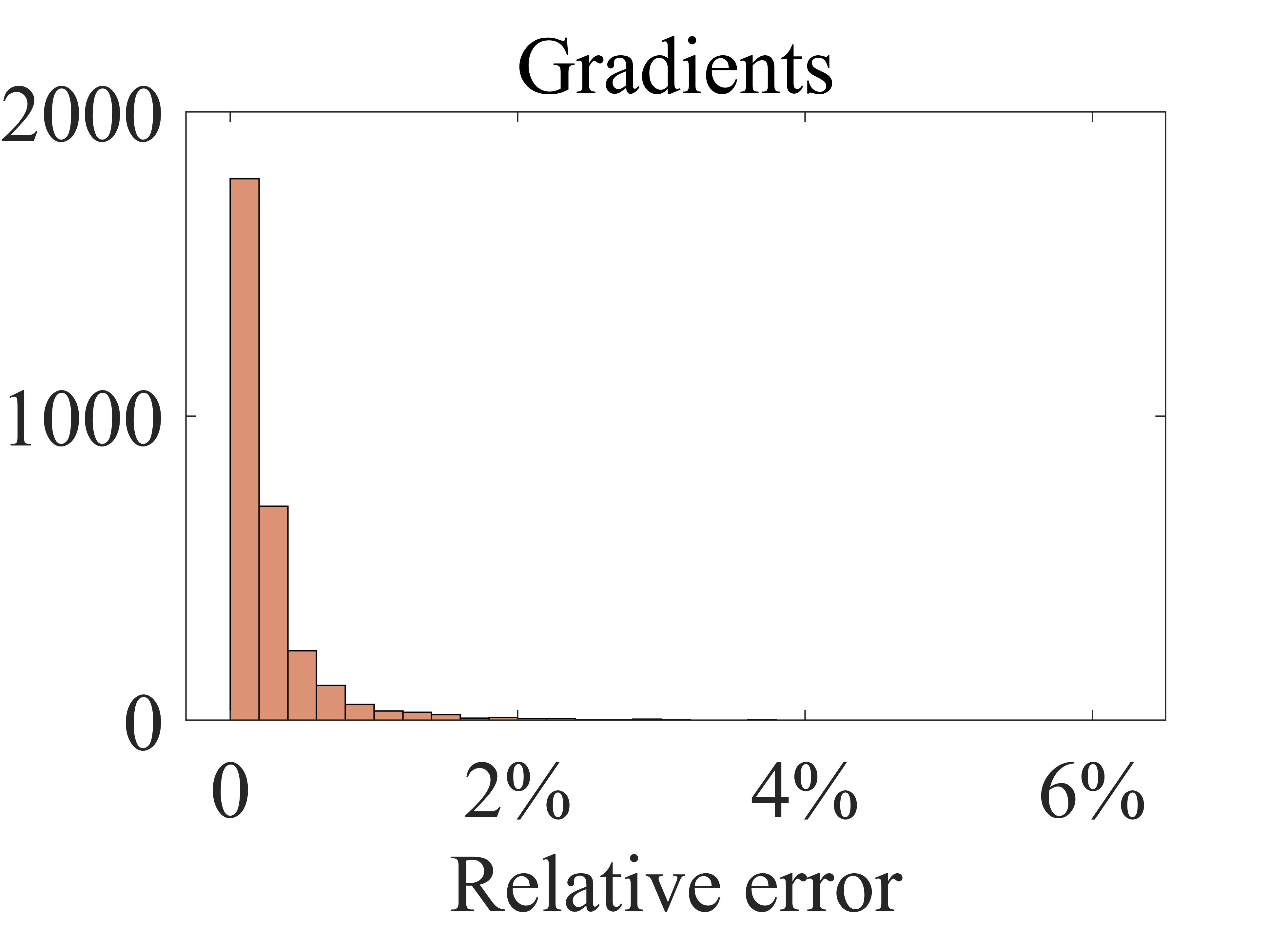
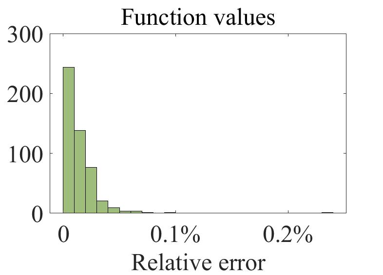
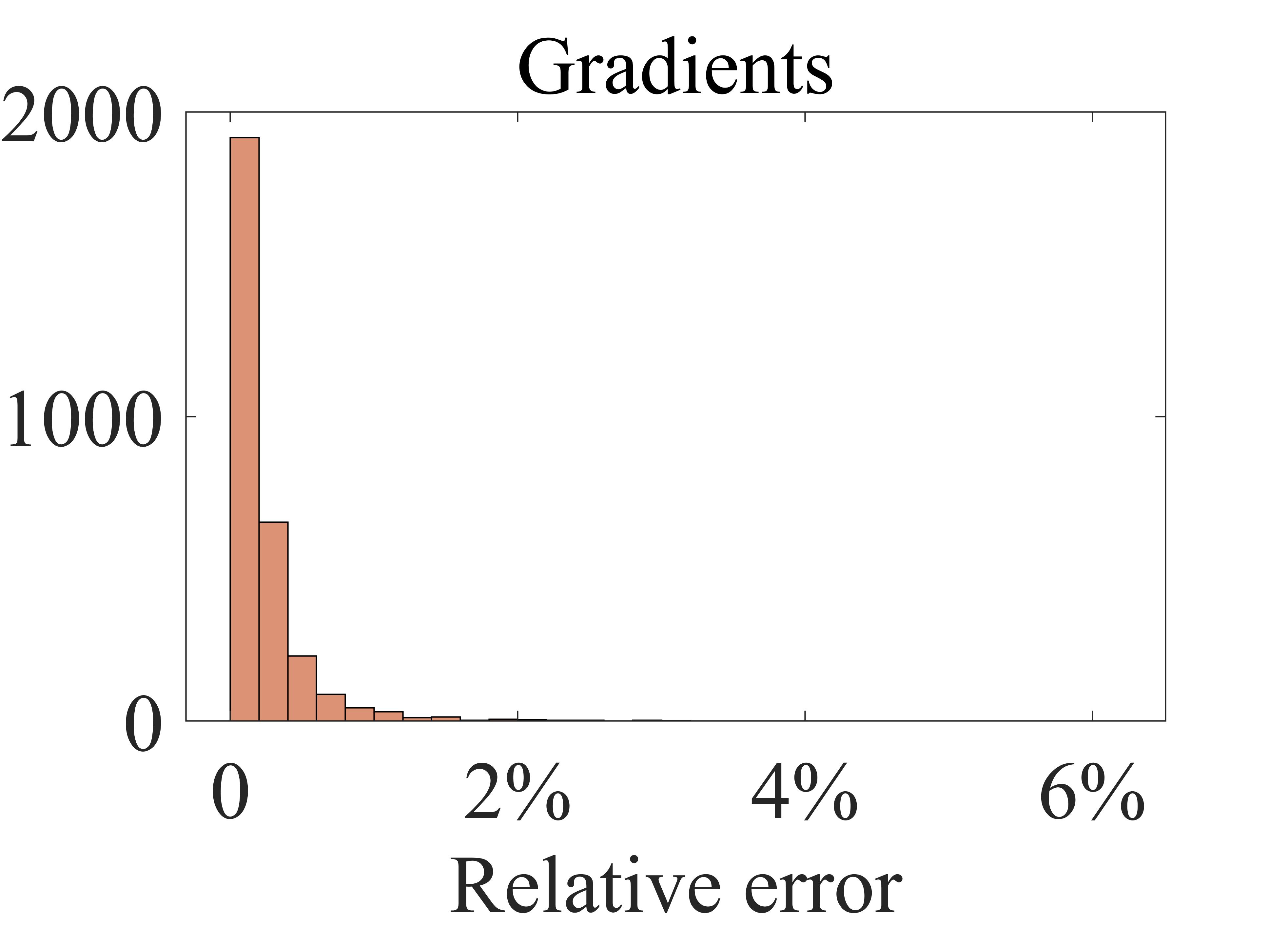
The experimental results are shown in Table 1, where we observe consistently small errors from the partial derivatives, albeit not included in the loss functions. For a more detailed discussion, we also show the distributions of the relative errors of function value and first-order partial derivatives in Fig. 3. For $f_{1}$, the maximum relative error is $0.11\%$, but most of the relative errors of function value are within $0.05\%$. The maximum relative error of the first-order partial derivatives is $6.15\%$, but $99.03\%$ of them are within $2\%$. On the other hand, for $f_{2}$, the maximum relative error is $0.24\%$, but $96\%$ of the relative errors of function value are within $0.04\%$. The maximum relative error of the first-order partial derivatives is $6.03\%$, but $98.77\%$ of them are within $1.5\%$. From these experimental results, we see that after fitting GNN to the function value, it can not only faithfully represent a multi-variable function but also well approximate its first-order partial derivatives.

Motivated by the above theoretic result, we propose to directly fit a GNN to the max-flow of the network and determine the update directions of the relay nodes by differentiating the GNN, as shown in Fig. 4. Unlike the naïve method of learning gradients, the learning objective of this approach is the scalar max-flow value of the network, which replaces the original node-level task to a graph-level task.

After we fit the GNN to the max-flow value, the test phase is conducted as follows. First, the graph representations ${\mathcal{G}}({\mathcal{V}},{\mathcal{E}},{\bm{A}})$ of test node locations are fed into the trained GNN. Then, we perform auto-differentiation to obtain the gradients of the output with respect to both the node features ${\bm{X}}$ and the weighted adjacency matrix ${\bm{A}}$

where $\left\langle\cdot,\cdot\right\rangle$ is the Hilbert-Schmidt inner product and

Here, $\displaystyle\frac{\partial A_{p,q}}{\partial x_{i}^{(m)}}$ depends on the network of interest and an example is given in Section 6.1. Finally, the relay nodes are updated along these directions with stepsize $\zeta$ as follows

where $\partial_{i}^{(m)}g={\partial g}/{\partial x_{i}^{(m)}}$.

To further improve the performance of throughput optimization, we also study a hybrid method based on an existing method [11] and the proposed MFL method.

To train GNN to learn the value of $C$ (or, equivalently, the max-flow), it is vital to create a dataset that well represents max-flow values for different node locations. In particular, it is important that the training dataset contains some node locations corresponding to good max-flow values, so that the GNN will not underestimate the maximum possible value of the max-flow of the network. To this end, we propose to use a reinforcement learning model based on a GNN implementation of PPO [50, 51] to obtain suitable training samples. This algorithm has a strong exploration capability to find the node locations corresponding to some good max-flow values in the sampling space.²² 2 We remark that PPO could also be used for optimizing the max-flow directly, but we don’t expect a good performance due to the complexity of the search space (see Section 6.4.2 for a comparison of performance). Therefore, the application of PPO is only regarded as a pre-training step which provides us with a good variety of training data.

In our context, the three key elements of the PPO algorithm are defined as follows:

• •

  state ($s$): the graph-structured data including node features ${\bm{X}}$ and edge features ${\bm{A}}$;

• •

  action ($a$): a collection of two-dimensional vectors representing the update directions of the relay nodes;

• •

  reward ($r$): the increment of the max-flow by taking an action at a given state.

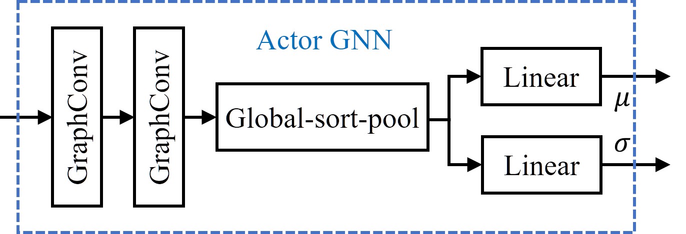
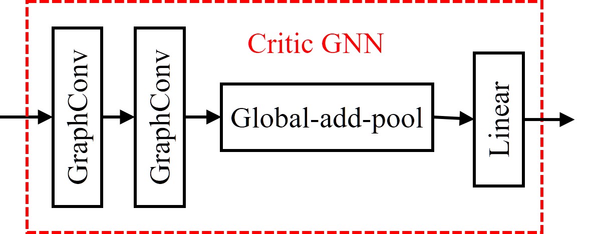
The agent in the PPO algorithm consists of an actor (i.e. the policy) and a critic (i.e. the value function), both modeled as GNNs. The actor GNN provides a policy for choosing an action for a given state, while the critic GNN evaluates possible cumulative rewards for a state. In particular, given a current state as the input, the outputs of the actor GNN are used as means and variances of $(n-2)\times 2$ normal distributions $\mathrm{Norm}(\mu_{i,l},\sigma_{i,l})$, $i=2,\dots,n-1$, $l=1,2$. The update of the relay node ${\bm{\xi}}_{i}$, $i=2,\dots,n-1$, is then a vector $(\Delta x_{i,1},\Delta x_{i,2})$, sampled according to $\Delta x_{i,1}\sim\mathrm{Norm}(\mu_{i,1},\sigma_{i,1})$ and $\Delta x_{i,2}\sim\mathrm{Norm}(\mu_{i,2},\sigma_{i,2})$. On the other hand, the critic GNN outputs a deterministic scalar value as the cumulative rewards.

The PPO algorithm runs for $N$ epochs, and each epoch is divided into $T$ timeslots. Here $T$ is equal to the product of the number of update steps $\mathfrak{T}$ and the number of updates from scratch $\varphi$. For the $i$-th epoch, $i=1,2,\dots,N$, we use $\pi_{\theta_{i}}$ to denote the actor GNN and $V_{\phi_{i}}$ to denote the critic GNN, where $\theta_{i}$ and $\phi_{i}$ denote the parameters in these two GNNs, respectively. We also use $s_{t}$, $a_{t}$, and $r_{t}$ to denote the state, action, and reward at the $t$-th timeslot, $t=1,2,\dots,T$, respectively, where for brevity we omit their dependence on $i$. Moreover, let $\pi_{\theta_{i}}\left(a_{t}|s_{t}\right)$ denote the probability that the policy $\pi_{\theta_{i}}$ executes $a_{t}$ at a given $s_{t}$, and $s^{\prime}_{t}$ denote the state after executing $a_{t}$ at $s_{t}$. With the above notations, we can represent the advantage $A_{t}\left(\theta_{i}\right)$ as

where $V_{\phi_{i}}\left(s_{t}\right)$ is the current value function from the critic GNN, and

Here, $\gamma$ is a hyperparameter. Accordingly, the loss function for updating the actor GNN is defined as

where $\mathbb{E}\left[\cdot\right]$ is the empirical average over all samples in the buffer (stored the training data of PPO), $\tau$ is a hyperparameter, and $\mathrm{clip}(\cdot,\cdot,\cdot,\cdot)$ is a clipping function defined as

and $\rho_{t}$ is a quotient of probability densities defined as

On the other hand, the loss function for updating the critic GNN is defined as

where $\mathfrak{L}$ is a piecewise function on $\mathbb{R}$ defined as

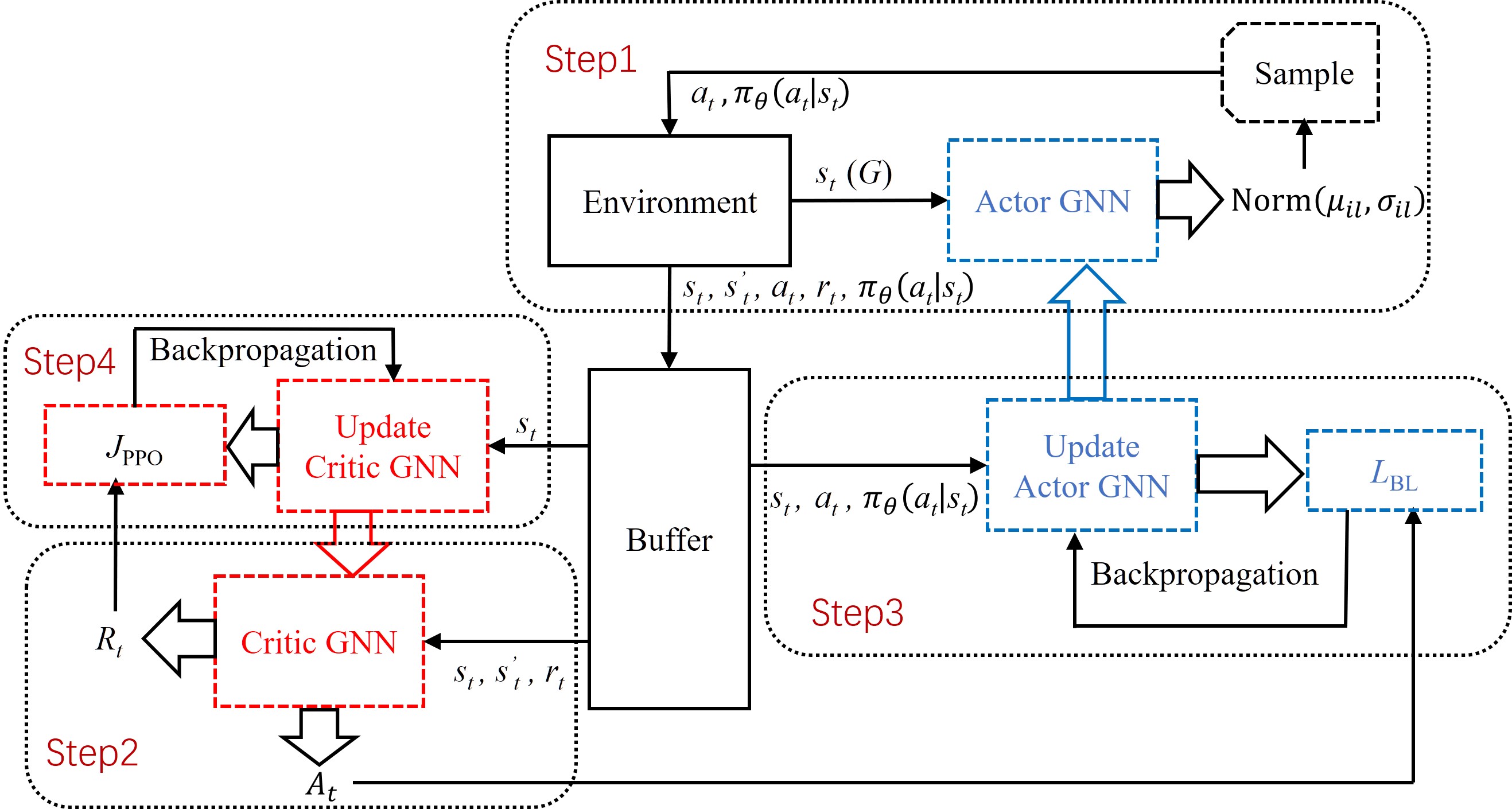
For clarity, we summarize the above procedures in Algorithm 1 and Fig. 6. Based on this framework, we explore the state space in a comprehensive way so that a sufficiently rich collection of update trajectories of the relay nodes can be obtained. Each trajectory $\{({\bm{\xi}}_{1}[\mathfrak{t}],{\bm{\xi}}_{2}[\mathfrak{t}],\dots,{\bm{\xi}}_{n}[\mathfrak{t}]),\mathfrak{t}=0,\dots,\mathfrak{T}\}$ consists of the positions of legitimate nodes that are updated $\mathfrak{T}$ times. To construct the training dataset, we collect data points $\{({\bm{\xi}}_{1}[{\mathfrak{t}}{k}],{\bm{\xi}}_{2}[{\mathfrak{t}}{k}],\dots,{\bm{\xi}}_{n}[{\mathfrak{t}}{k}]),\mathfrak{t}=0,\dots,\mathfrak{T}/k\}$ along each trajectory at a fixed time interval $k$.

We test our methodology in the scenario where, in addition to a wireless network with the source, destination, and relay nodes (which will be referred to as legitimate nodes altogether), there also exists a jammer. Note that similar anti-jamming communication scenarios are commonly considered in the wireless communication literatures [9, 52, 11, 12]. In the considered scenario, the jammer is assumed to be positioned at a known location ${\bm{\xi}}_{\rm J}=\left(x_{\rm J}^{(1)},x_{\rm J}^{(2)}\right)\in\mathbb{R}^{2}$ and it interferes the data transmission within the wireless network. The signal-to-interference ratio (SIR) for the transmission from node $i$ to node $j$, ${\rm SIR}_{i,j}$, $i,j\in\{1,\dots,n\}$ can be modelled as

where $d_{i,j}=\left\lVert{\bm{\xi}}_{i}-{\bm{\xi}}_{j}\right\rVert$ is the distance between node $i$ and node $j$, $d_{j,J}=\left\lVert{\bm{\xi}}_{j}-{\bm{\xi}}_{\rm J}\right\rVert$ is the distance between node $j$ and the jammer, $\eta$ is the power ratio of the jammer to the legitimate nodes. Note that, a path-loss model [53] for the wireless channel is assumed in (31) and $\alpha$ is the path loss factor, and $r_{\rm int}$ is a design parameter. Also, $\Xi_{i,j}=\{1,\dots,n\}\backslash\{i,j\}$, where “$\backslash$” denotes set difference, is the set of indices of legitimate nodes excluding $i$ and $j$. To prevent violation of physical constraints, $\nu$ is defined by

where $\varrho$ and $\kappa$ are all design parameters, and $z_{0}$ can be an arbitrarily small positive number. Based on the above model, the (two-way average) communication rate $f_{\rm cap}$ in (1) between two nodes $i$ and $j$ is defined as

where it is assumed that orthogonal spectrum is allocated to each link of the network and $B$ denotes the corresponding bandwidth per link. Therefore, the corresponding derivatives $\displaystyle\frac{\partial A_{p,q}}{\partial x_{i}^{(m)}}$ (cf. (22)) for this considered scenario can be found by the chain rule based on (31)–(33).

In our experiments, we consider a wireless network with $n=6$ legitimate nodes in a $600\times 600~m^{2}$ area. We represent this area by a Cartesian coordinate system, where the range of $x$-coordinate is $\left(-6,6\right)$ and the range of $y$-coordinate is $\left(-6,6\right)$, and the unit length in both coordinates is set to 50 meters. The coordinates of the source and the destination nodes are fixed to ${\bm{\xi}}_{1}=(-4.5,0)$ and ${\bm{\xi}}_{6}=(4.5,0)$, respectively. In each deployment, the relay nodes are initialized with the following coordinates: ${\bm{\xi}}_{2}=(-2.7,0)$, ${\bm{\xi}}_{3}=(-0.9,0)$, ${\bm{\xi}}_{4}=(0.9,0)$, ${\bm{\xi}}_{5}=(2.7,0)$. The coordinates of the jammer node are randomly chosen with the following constraints: $x_{\rm J}^{(1)}\in\left(-6,6\right),x_{\rm J}^{(2)}\in\left(-6,6\right),d_{1,{\rm J}}>3,$ and $d_{6,\rm{J}}>3$, where the last two constraints represent “guard zones” that prevent the jammer from getting too close to the source or destination.

To generate the training set, we initialize a total of $2,000$ deployments. Every deployment is updated for $\mathfrak{T}=400$ steps with stepsize $\zeta=0.02$ following the PPO strategy described in Section 5.3. In the GNN-based PPO, we choose $\gamma=0.9$, $\tau=0.2$, $\varphi=5$, $T=400\times 5=2,000$, $M=10$. We collect a data point once every $5$ steps from each deployment. For convenience, we name this dataset the RLGP (short for Reinforcement Learning GNN-PPO) dataset. For efficiency, the actor GNN and the critic GNN stop training when the reward converges or the number of epochs reaches the maximum. On the other hand, the test set contains $500$ initial deployments which have different jammer locations.

We used the PyTorch Geometric library [54] to implement all the GNN-related tasks.

We compare MFL with the following baseline methods.

• •

  Gradient Learning (GL): This baseline is the naïve approach introduced in Section 3.2. The GNNs in both MFL and GL are trained using the RLGP dataset described in Section 6.1. The label for MFL is the max-flow value, while the labels for GL are the directions of the relay nodes traveled in the training procedure.

• •

  Reinforcement Learning (RL): This baseline is a direct application of PPO to the test data. Specifically, we train an agent to explore the test data and provide the update directions for the relay nodes. The training procedure still follows the framework illustrated in Fig. 6. We obtain the optimal trajectory of each test deployment and use it to compare with MFL. To ensure good results, the number of timeslots, $T$, is chosen to be $40,000$, and the number of epochs, $N$, is $10,000$.

• •

  Weighted Cheeger Constant (WCC): This baseline is introduced in Section 5.2.1. As in the CC method, we use the gradients of $\lambda_{2}({\bm{L}}_{{\bm{W}}})$ to adjust the locations of relay nodes. In our experiments, the weight matrix is ${\bm{W}}={\rm diag}\{w_{1},\dots,w_{n}\}$, where $w_{i}=3n$ if $i=1,n$, and $w_{i}=1$ if $i\neq 1,n$.

In our experiments, we use several different GNNs. We describe their structures as follows.

We use the same test set described in Section 6.1 to evaluate the performance of all baseline methods mentioned above. In Fig. 10, we illustrate an example showing the trace of updates during the testing process, where the relay nodes are updated for $\mathfrak{T}=400$ steps. The corresponding change of the max-flow value of this network is shown in Fig. 10. The performance of the methods is measured by the final max-flow of the network after the relay node location update.

We present the experimental results of the hybrid method in Fig. 14.

The performance of the hybrid method excels both individual approaches. Compared with the MFL method, the hybrid method is superior in $418$ test deployments. Fig. 14 reveals that although most of the data only see an improvement of $20\%$ or less, there were still some deployments with an improvement of $50\%$ or more, with the largest reaching $641\%$. In Fig. 14, we observe that some deployments for which the MFL method does not perform well have an improved result when we use the hybrid method. On the other hand, as observed in Fig. 14, $94\%$ of the test data enjoy improved results when the hybrid method replaces the WCC method. Although the hybrid method performs well, Fig. 14 shows clearly that there are still specific regions of the jammer node where the hybrid method falls behind the WCC method. We believe the hybrid method does not completely resolve the problem at the edge of guard zones, from which the MFL method suffers.

To summarize the results more clearly, we use the WCC method as a benchmark to quantitatively compare the average performance in the test set. We show the average difference of the max-flow (avg. diff. mf.) and the average relative difference (avg. rel. diff. mf.) in Table 3. In addition, to eliminate the influence of outliers, we calculate the truncated-averaged difference (c-avg. diff. mf.) and the truncated-averaged relative difference (c-avg. rel. diff. mf.), excluding the highest and lowest $10\%$ values. In all these metrics, the hybrid method has the best overall performance.

We perform ablation studies to show two important ideas implemented in our experiments. The first is the use of reinforcement learning for generating the dataset; the second is the use of expressive GNN layers throughout our experiments.

References

- [1] W. H. Chin, Z. Fan, and R. Haines, “Emerging technologies and research challenges for 5G wireless networks,” IEEE Wireless Commun., vol. 21, no. 2, pp. 106–112, 2014.
- [2] A. K. Gupta, X. Zhang, and J. G. Andrews, “SINR and throughput scaling in ultradense urban cellular networks,” IEEE Wireless Commun. Lett., vol. 4, no. 6, pp. 605–608, 2015.
- [3] T.-J. Wu, W. Liao, and C.-J. Chang, “A cost-effective strategy for road-side unit placement in vehicular networks,” IEEE Trans. Commun., vol. 60, no. 8, pp. 2295–2303, 2012.
- [4] X. You, H. Yin, and H. Wu, “On 6G and wide-area IoT,” Chin. J. Internet Things, vol. 4, no. 1, pp. 3–11, 2020.
- [5] A. Merwaday and I. Guvenc, “UAV assisted heterogeneous networks for public safety communications,” in Proc. IEEE Wireless Commun. Netw. Conf. (WCNC), 2015, pp. 329–334.
- [6] H. Wang, X. Zhou, and M. C. Reed, “Coverage and throughput analysis with a non-uniform small cell deployment,” IEEE Trans. Wireless Commun., vol. 13, no. 4, pp. 2047–2059, 2014.
- [7] D. H. Kang, K. W. Sung, and J. Zander, “Attainable user throughput by dense Wi-Fi deployment at 5 GHz,” in Proc. IEEE PIMRC, 2013, pp. 3418–3422.
- [8] J. Lyu and R. Zhang, “Spatial throughput characterization for intelligent reflecting surface aided multiuser system,” IEEE Wireless Commun. Lett., vol. 9, no. 6, pp. 834–838, 2020.
- [9] H. Wang, J. Chen, G. Ding, and J. Sun, “Trajectory planning in UAV communication with jamming,” in Proc. Int. Conf. Wireless Commun. Signal Process. (WCSP), 2018, pp. 1–6.
- [10] S.-F. Chou, A.-C. Pang, and Y.-J. Yu, “Energy-aware 3D unmanned aerial vehicle deployment for network throughput optimization,” IEEE Trans. Wireless Commun., vol. 19, no. 1, pp. 563–578, 2019.
- [11] X. He, H. Dai, and P. Ning, “Dynamic adaptive anti-jamming via controlled mobility,” IEEE Trans. Wireless Commun., vol. 13, no. 8, pp. 4374–4388, 2014.
- [12] A. Rahmati, S. Hosseinalipour, Y. Yapici, X. He, I. Guvenc, H. Dai, and A. Bhuyan, “Dynamic interference management for UAV-assisted wireless networks,” IEEE Trans. Wireless Commun., 2021.
- [13] P. Yang, X. Cao, X. Xi, Z. Xiao, and D. Wu, “Three-dimensional drone-cell deployment for congestion mitigation in cellular networks,” IEEE Trans. Veh. Technol., vol. 67, no. 10, pp. 9867–9881, 2018.
- [14] M. Mozaffari, W. Saad, M. Bennis, and M. Debbah, “Efficient deployment of multiple unmanned aerial vehicles for optimal wireless coverage,” IEEE Commun. Lett., vol. 20, no. 8, pp. 1647–1650, 2016.
- [15] M. Chen, M. Mozaffari, W. Saad, C. Yin, M. Debbah, and C. S. Hong, “Caching in the sky: Proactive deployment of cache-enabled unmanned aerial vehicles for optimized quality-of-experience,” IEEE J. Select. Areas Commun., vol. 35, no. 5, pp. 1046–1061, 2017.
- [16] Z. Wu, S. Pan, F. Chen, G. Long, C. Zhang, and S. Y. Philip, “A comprehensive survey on graph neural networks,” IEEE Trans. Neural Netw. Learn. Syst., vol. 32, no. 1, pp. 4–24, 2020.
- [17] S. Abadal, A. Jain, R. Guirado, J. López-Alonso, and E. Alarcón, “Computing graph neural networks: A survey from algorithms to accelerators,” ACM Comput. Surv., vol. 54, no. 9, pp. 1–38, 2021.
- [18] X. Zhang, H. Zhao, J. Xiong, X. Liu, L. Zhou, and J. Wei, “Scalable power control/beamforming in heterogeneous wireless networks with graph neural networks,” in Proc. IEEE Glob. Commun. Conf., 2021, pp. 01–06.
- [19] M. Eisen and A. Ribeiro, “Optimal wireless resource allocation with random edge graph neural networks,” IEEE Trans. Signal Process., vol. 68, pp. 2977–2991, 2020.
- [20] J. Guo and C. Yang, “Learning power control for cellular systems with heterogeneous graph neural network,” in Proc. IEEE Wireless Commun. Netw. Conf., 2021, pp. 1–6.
- [21] O. Orhan, V. N. Swamy, T. Tetzlaff, M. Nassar, H. Nikopour, and S. Talwar, “Connection management xAPP for O-RAN RIC: A graph neural network and reinforcement learning approach,” in Proc. IEEE Int. Conf. Mach. Learn. Appl., 2021, pp. 936–941.
- [22] S. Moon, S. Ahn, K. Son, J. Park, and Y. Yi, “Neuro-DCF: Design of Wireless MAC via Multi-Agent Reinforcement Learning Approach,” in Proc. ACM Mobihoc, 2021, pp. 141–150.
- [23] J. Bruna, W. Zaremba, A. Szlam, and Y. LeCun, “Spectral networks and locally connected networks on graphs,” in Proc. Int. Conf. Learn. Represent., 2020.
- [24] R. Kondor, T. S. Hy, H. Pan, B. M. Anderson, and S. Trivedi, “Covariant compositional networks for learning graphs,” in Proc. Int. Conf. Learn. Represent. Workshop, 2018.
- [25] D. Zou and G. Lerman, “Graph convolutional neural networks via scattering,” Appl. Comput. Harmon. Anal., vol. 49, no. 3, pp. 1046–1074, 2020.
- [26] N. Keriven and G. Peyré, “Universal invariant and equivariant graph neural networks,” Proc. NeurIPS, vol. 32, 2019.
- [27] H. Maron, H. Ben-Hamu, N. Shamir, and Y. Lipman, “Invariant and equivariant graph networks,” arXiv:1812.09902., 2018. [Online]. Available: https://arxiv.org/abs/1812.09902
- [28] K. Hornik, “Approximation capabilities of multilayer feedforward networks,” Neural Netw, vol. 4, no. 2, pp. 251–257, 1991.
- [29] Z. Chen, S. Villar, L. Chen, and J. Bruna, “On the equivalence between graph isomorphism testing and function approximation with gnns,” in Proc. NeurIPS, 2019, pp. 15 894–15 902.
- [30] K. Xu, W. Hu, J. Leskovec, and S. Jegelka, “How powerful are graph neural networks?” in Proc. Int. Conf. Learn. Represent., 2019.
- [31] C. Morris, M. Ritzert, M. Fey, W. L. Hamilton, J. E. Lenssen, G. Rattan, and M. Grohe, “Weisfeiler and leman go neural: Higher-order graph neural networks,” in Proc. AAAI Conf. Artif. Intell., vol. 33, no. 01, 2019, pp. 4602–4609.
- [32] C. Bodnar, F. Frasca, Y. Wang, N. Otter, G. F. Montufar, P. Lio, and M. Bronstein, “Weisfeiler and lehman go topological: Message passing simplicial networks,” in Proc. Int. Conf. Mach. Learn., 2021, pp. 1026–1037.
- [33] H. Maron, E. Fetaya, N. Segol, and Y. Lipman, “On the universality of invariant networks,” in Proc. Int. Conf. Mach. Learn., 2019, pp. 4363–4371.
- [34] T. Nguyen-Thien and T. Tran-Cong, “Approximation of functions and their derivatives: A neural network implementation with applications,” Appl. Math. Model., vol. 23, no. 9, pp. 687–704, 1999.
- [35] W. M. Czarnecki, S. Osindero, M. Jaderberg, G. Swirszcz, and R. Pascanu, “Sobolev training for neural networks,” in Proc. NeurIPS, 2017, pp. 4281–4290.
- [36] N. N. Vlassis and W. Sun, “Sobolev training of thermodynamic-informed neural networks for interpretable elasto-plasticity models with level set hardening,” Comput. Methods Appl. Mech. Eng., vol. 377, p. 113695, 2021.
- [37] H. Son, J. W. Jang, W. J. Han, and H. J. Hwang, “Sobolev training for the neural network solutions of pdes,” arXiv:2101.08932., 2021. [Online]. Available: https://arxiv.org/abs/2101.08932
- [38] L. R. Ford and D. R. Fulkerson, “Maximal flow through a network,” Can. J. Math., vol. 8, pp. 399–404, 1956.
- [39] H. Kim, G. Papamakarios, and A. Mnih, “The lipschitz constant of self-attention,” in Proc. Int. Conf. Mach. Learn., 2021, pp. 5562–5571.
- [40] H. Federer, Geometric measure theory. Springer, 2014.
- [41] K. Hornik, M. Stinchcombe, and H. White, “Multilayer feedforward networks are universal approximators,” Neural Netw, vol. 2, no. 5, pp. 359–366, 1989.
- [42] S. C. Brenner, L. R. Scott, and L. R. Scott, The mathematical theory of finite element methods. Springer, 2008, vol. 3.
- [43] J. He, L. Li, J. Xu, and C. Zheng, “ReLU deep neural networks and linear finite elements,” J. Comput. Math., vol. 38, no. 3, pp. 502–527, 2020.
- [44] W. Azizian and marc lelarge, “Expressive Power of Invariant and Equivariant Graph Neural Networks,” in Proc. Int. Conf. Learn. Represent., 2021.
- [45] S. Jegelka, “Theory of Graph Neural Networks: Representation and Learning,” arXiv:2204.07697., 2022. [Online]. Available: https://arxiv.org/abs/2204.07697
- [46] D. Hendrycks and K. Gimpel, “Gaussian error linear units (gelus),” arXiv:1606.08415., 2016. [Online]. Available: https://arxiv.org/abs/1606.08415
- [47] V. P. Dwivedi, C. K. Joshi, T. Laurent, Y. Bengio, and X. Bresson, “Benchmarking graph neural networks,” arXiv:2003.00982., 2020. [Online]. Available: https://arxiv.org/abs/2003.00982
- [48] J. Sherman, “Breaking the multicommodity flow barrier for O ()-approximations to sparsest cut,” in Proc. 50th Annu. IEEE Symp. Found. Comput. Sci. (FOCS), 2009, pp. 363–372.
- [49] S. Bhattacharya and T. Başar, “Graph-theoretic approach for connectivity maintenance in mobile networks in the presence of a jammer,” in Proc. IEEE CDC, 2010, pp. 3560–3565.
- [50] J. Schulman, F. Wolski, P. Dhariwal, A. Radford, and O. Klimov, “Proximal policy optimization algorithms,” arXiv:1707.06347., 2017. [Online]. Available: https://arxiv.org/abs/1707.06347
- [51] N. Heess, D. TB, S. Sriram, J. Lemmon, J. Merel, G. Wayne, Y. Tassa, T. Erez, Z. Wang, S. M. A. Eslami, M. A. Riedmiller, and D. Silver, “Emergence of locomotion behaviours in rich environments,” arXiv:1707.02286., 2017. [Online]. Available: https://arxiv.org/abs/1707.02286
- [52] I. Valiulahi and C. Masouros, “Multi-UAV deployment for throughput maximization in the presence of co-channel interference,” IEEE Internet Things J., vol. 8, no. 5, pp. 3605–3618, 2020.
- [53] D. K. Goldenberg, J. Lin, A. S. Morse, B. E. Rosen, and Y. R. Yang, “Towards mobility as a network control primitive,” in Proc. ACM Mobihoc, 2004, pp. 163–174.
- [54] M. Fey and J. E. Lenssen, “Fast graph representation learning with PyTorch Geometric,” in Proc. ICLR Workshop Representation Learn. Graphs Manifolds, 2019.